Modelling the dynamics of implied volatility smiles and surfaces

University of Warwick institutional repository: http://go.warwick.ac.uk/wrap

A Thesis Submitted for the Degree of PhD at the University of Warwick

http://go.warwick.ac.uk/wrap/65194

This thesis is made available online and is protected by original copyright. Please scroll down to view the document itself.

MODELLING THE DYNAMICS OF IMPLIED

VOLATILITY SMILES AND SURFACES

Georgios Sldadopoulos

Thesis submitted in fulfilment of the requirements for the Degree of

Doctor of Philosophy in Finance

University of Warwick,

Warwick Business School

Contents

1 Introduction

2 Literature Review 2.1 Introduction..

2.2 Smile Consistent Deterministic Volatility Models in Continuous Time

2.2.1 Theoretical Justifications for "Smile-Consistent" Deterministic Volatility Models

2.2.2 Dupire (1993 and 1994) 2.3 Smile Consistent

Models in Discrete Time

2.3.1 Derman and Kani (1994) . 2.3.2 Barle and Cakici (1995) 2.3.3 Rubinstein (1994) . 2.3.4 Jackwerth (1997) 2.3.5 Trinomial Trees.

Deterministic

2.3.6 Implicit Finite Difference Schemes . 2.4 Testing the Validity

Volatility Assumption. 2.5 Smile Consistent

Volatility Models . . 2.5.1 Dupire (1992)

No

of the

Arbitrage

Volatility

Deterministic

.

...

Stochastic 17

21 21

23

24 25

28 29 32 33 35 36 39

40

".42

2.5.3 Derman and Kani (1998) . . . . 2.5.4 Extracting the Local Volatility Surface 2.5.5 Britten-Jones and Neuberger (1998) . 2.5.6 Ledoit and Santa-Clara (1998) . 2.6 Concluding Remarks . . . .

3 Description and Screening of the Data Set 3.1 Introduction.

3.2 The Data Set

3.3 The Calculation of Implied Volatilities 3.4 Screening the Data . . . .

3.4.1 Screening the raw Data. 3.4.2 Screening Implied Volatilities 3.4.3 The Vega Constraint

3.5 Summary . . . .

4 The Dynamics of Smiles 4.1 Introduction...

51 53 55 58 59

61 61 61 62 65 65 66 68 75

76 76 4.2 Principal Components Analysis and Implied Volatilities. 78 4.2.1 Description of the Principal Components Analysis. 78 4.2.2 The Metrics . . . 80 4.2.3 The Determination of the Expiry Buckets 82

4.3 PCA on the Strike Metric . . . 84

4.3.1 Choosing the Strike Variables

4.3.2 Some Descriptives for the chosen Variables

4.3.3 Number of Retained Principal Components and a First In-terpretation . . . .

4.3.4 The Rotation Method 4.4 PCA on the Moneyness Metric.

4.4.1 Construction of the Moneyness Metric 4.4.2 Some Descriptives for the Chosen variables.

84 85

4.4.3 Number of Retained Principal Components and a First In-terpretation . . . .

4.4.4 The Rotation Method 4.5 Serial Correlation

Differences . 4.6 Comparing

Metrics . . .

the

and

Results

the use of the

from the Two

4.7 Correlations between the FUtures Price and the Principal Compo-124 138

146

147

nents . . . . 149

4.8 Conclusions 153

5 The Dynamics of Implied Volatility Surfaces 155

5.1 Introduction... 155

5.2 PCA on the Strike Metric 156

5.2.1 Determining the Expiry Buckets. 156

5.2.2 Number of Retained Principal Components and a First In-terpretation . . . .

5.2.3 Interpretation of the Rotated Components

157 164

5.3 PCA on the Moneyness Metric. 168

5.3.1 Preliminary Descriptives 168

5.3.2 Number of Retained Principal Components and a First In-terpretation . . . .

5.3.3 Interpretation of the Rotated Components

5.4 Comparing the Results from the

Metrics . . .

Two

5.5 Correlations of the Changes of the FUtures Price with the Changes of the PCs under the Two Metrics .

5.6 Conclusions . . . .

6 A New Method for Simulating the Evolution of the Implied Dis-169 175

179

181 181

6.1 Introduction .

.

. .

. .

.

. . ...

185

6.2 Simulation of Implied Distributions and

Option Pricing

.

. . . .

. .

...

.

.

188 6.3 Partitions, Mixtures, and the Simulation of the Implied

Distribu-tion

...

189

6.3.1 Partitions and Mixtures 190

6.3.2 Simulating the Implied Distribution . 192 6.3.3 Inverting the Initial Implied Distribution 197

6.4 Simulating Changes in the Asset Price 198

6.4.1 The Algorithm

....

198

6.4.2 A Numerical Example 200

6.4.3 Checking the Accuracy of the Transformation 203 6.5 Simulation of the Implied Distribution when the Volatility Changes 205 6.5.1 The Algorithm . . . 205 6.5.2 Calculating the Mean and the Variance of the

Variance ..

6.5.3 Choosing a PDF for the Variance 6.5.4 A Numerical Example . . . . 6.6 Conclusions and Issues for Further Research

7 Conclusions and Suggested Future Research 7.1 ConcI usions . . .

7.2 Future Research .

206 208 209 213

215 215 216

A Explained Communalities in the Smile Analysis in the Strike

Metric 221

B Construction of the Procrustes Rotation Method 224

C Explained Communalities in the Smile Analysis in the

D Explained Communalities in the Surface Analysis in the Strike

Metric 231

E Explained Communalities in the Surface Analysis in the

Money-ness Metric 233

F The Moments of a Mixture of (Normal) Distributions, Mixed

across the Variance 235

G Constructing the Binomial Tree for the Evolution of the

LIST OF FIGURES

Figure Title Page

Chapter 3: Description and Screening of the Data Set

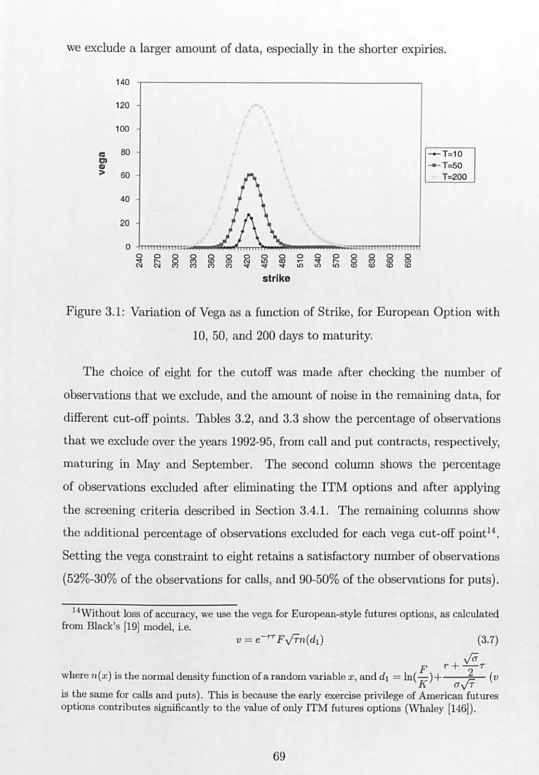
3.1 Variation of Vega as a function of Strike, for a European Option with 69 10, 50, and 200 days to maturity.

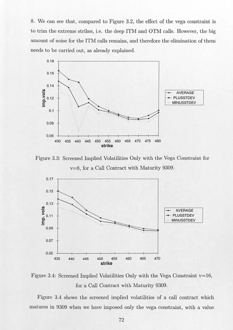
3.2 Raw Implied Volatilities for a Call Contract with Maturity 9309. 71 3.3 Screened Implied Volatilities Only with the Vega Constraint for v=8, 72

for a Call Contract with Maturity 9309.

3.4 Screened Implied Volatilities Only with the Vega Constraint v=16, for 72 a Call Contract with Maturity 9309.

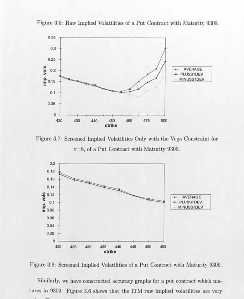
3.5 Screened Implied Volatilities for a Call Contract with Maturity 9309. 73 3.6 Raw Implied Volatilities of a Put Contract with Maturity 9309. 73 3.7 Screened Implied Volatilities Only with the Vega Constraint for v=8, 74

of a Put Contract with Maturity 9309.

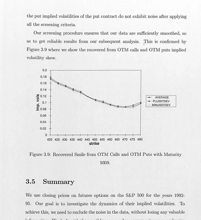
3.8 Screened Implied Volatilities of a Put Contract with Maturity 9309. 74 3.9 Recovered Smile from OTM Calls and OTM Puts with Maturity 9309. 75

Chapter 4: The Dynamics of Smiles 4.1 Smile Analysis on the Strike Metric Statistics

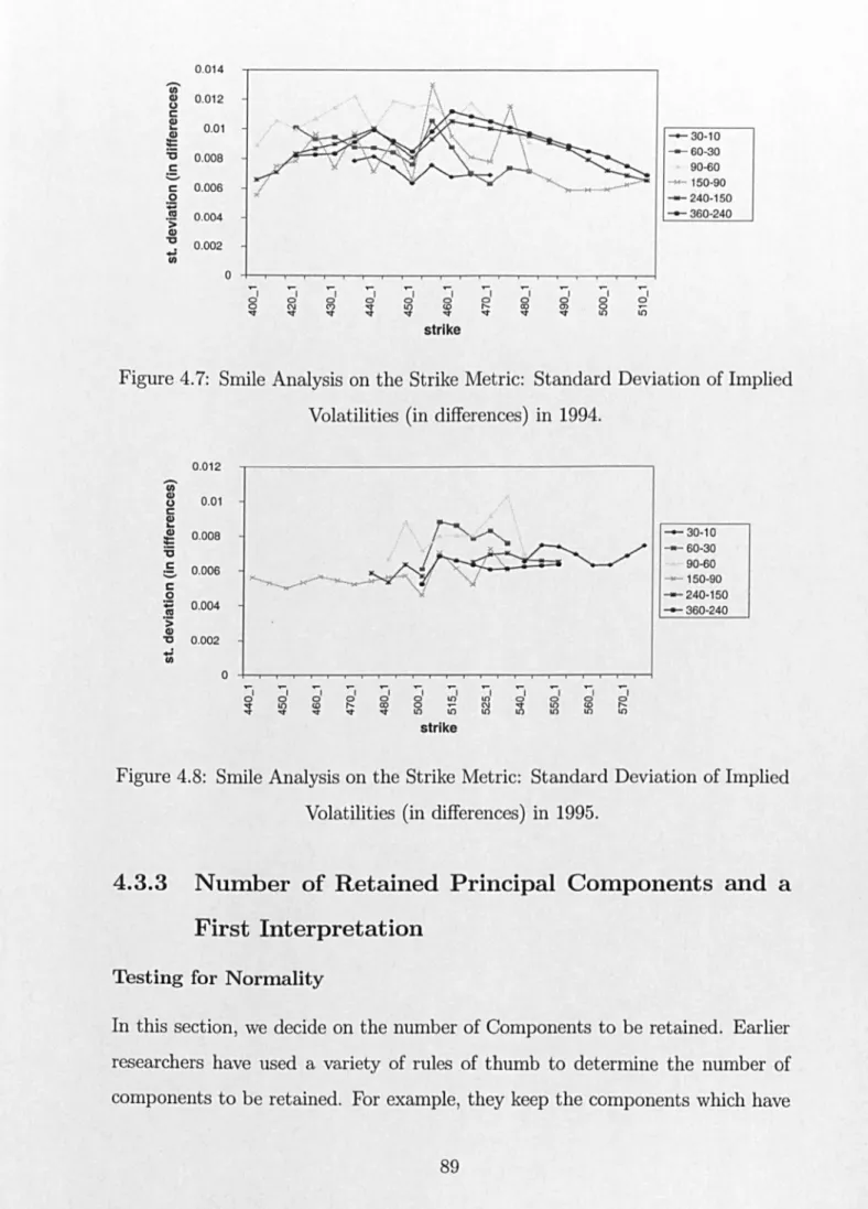
4.1-4.4 Average Implied Volatilities (levels) in 1992-95. 85,87 4.5-4.8 Standard Deviation of Implied Volatilities (in differences) in 1992-95. 88-89

4.9 Q-Q Plot for the First Differences of implied Volatilities in the 30-10 93 range, for the strike 540 for 1995

A First Interpretation of the PCs

4.10-4.15 Interpretation of the First PC for 30-10,60-30,90-60, 150-90,240-150, 98-100 360-240.

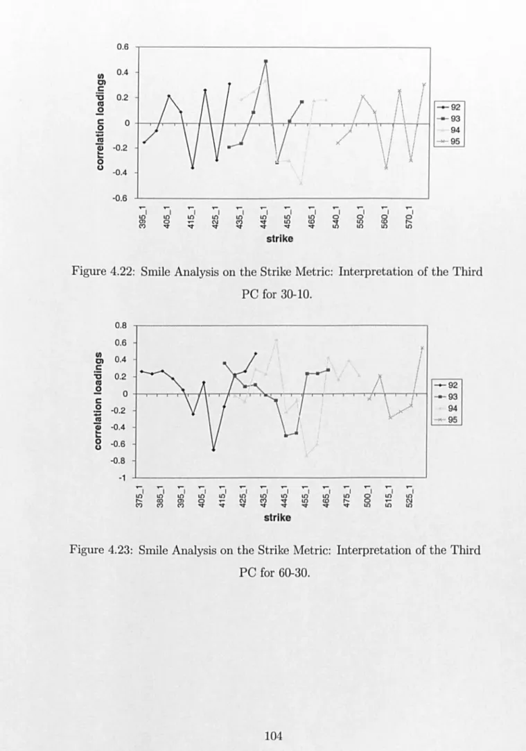
4.22-4.27 Interpretation ofthe Third PC for 30-10, 60-30, 90-60, 150-90, 240- 104-106 150, 360-240.

4.28 Rotated Correlation Loadings Obtained from Varimax Rotation, in the 109 60-30 Expiry, in Year 1992.

Interpretation of the Rotated PCs

4.29-4.34 Interpretation of the First Rotated PC for 30-10,60-30,90-60, 150-90, 111-113 240-150,360-240

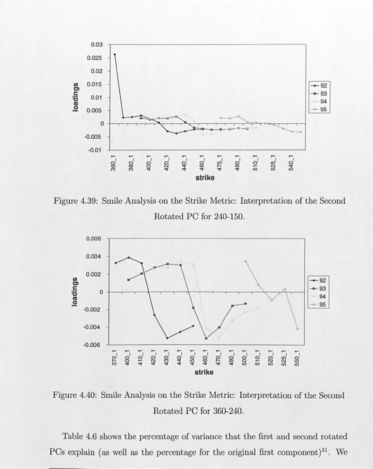
4.35-4.40 Interpretation of the Second Rotated PC for 30-10,60-30,90-60, 150- 114-116 90,240-150,360-240

4.2 Smile Analysis on the Moneyness Metric Statistics

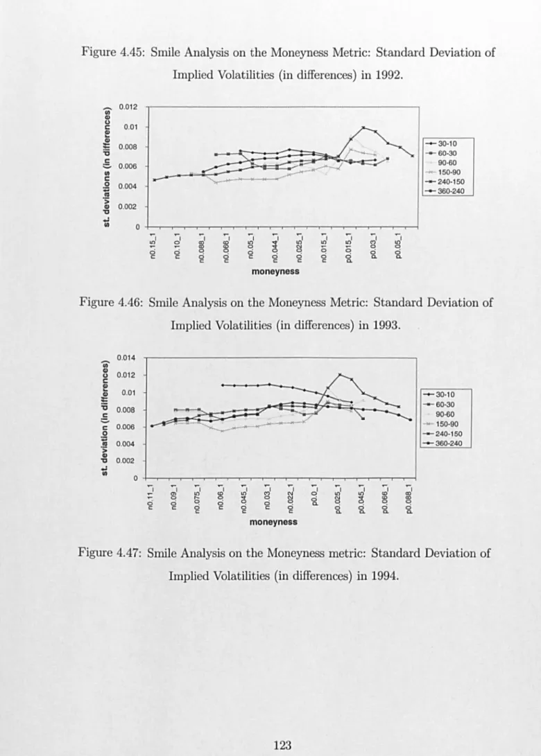
4.41-4.44 Average Implied Volatilities (levels) in 1992-95. 121-122 4.45-4.48 Standard Deviation of Implied Volatilities (in differences) in 1992-95. 122-124

4.49 Q-Q Plot for the First Differences of Implied Volatilities of 126 Moneyness -1.5% in the range 30-10, in year 1995.

A First Interpretation of the PCs

4.50-4.55 Interpretation of the First PC for 30-10,60-30,90-60, 150-90,240- 129-131 150,360-240.

4.56-4.61 Interpretation of the Second PC for 30-10, 60-30, 90-60, 150-90, 240- 132-134 150, 360-240.

4.62-4.67 Interpretation of the Third PC for 30-10, 60-30, 90-60, 150-90,240- 135-137 150, 360-240.

Interpretation of the Rotated PCs

4.68-4.73 Interpretation of the First Rotated PC for 30-10,60-30,90-60, 150-90, 139-141 240-150,360-240.

Chapter 5: The Dynamics of Implied Volatility Surfaces

5.1 Surface Analysis on the Strike Metric A First Interpretation of the PCs

5.1-5.3 Interpretation of the First PC for 90-10, 180-90, 270-180. 159-160 5.4-5.6 Interpretation of the Second PC for 90-10, 180-90, 270-180. 161-162 5.7-5.9 Interpretation of the Third PC for 90-10, 180-90, 270-180. 162-163

Interpretation of the Rotated PCs

5.10-5.12 Interpretation of the First Rotated PC for 90-10, 180-90, 270-180. 165-166 5.13-5.15 Interpretation of the Second Rotated PC for 90-10, 180-90, 270-180 166-167

5.2 Surface Analysis on the Moneyness Metric A First Interpretation of the PCs

5.16-5.18 Interpretation of the First PC for 90-10, 180-90, 270-180. 171-172 5.19-5.21 Interpretation of the Second PC for 90-10, 180-90,270-180. 172-173 5.22-5.24 Interpretation of the Third PC for 90-10, 180-90, 270-180. 174-175

Interpretation of the Rotated PCs

5.25-5.27 Interpretation of the First Rotated PC for 90-10, 180-90, 270-180. 176-177 5.28-5.30 Interpretation of the Second Rotated PC for 90-10, 180-90, 270-180. 177-178

Chapter 6: A New l\fethod for Simulating the Evolution of the Implied Distribution

6.1 Partitioning of the Original Distribution in two possible realizations. 191 6.2 Establishing the Mapping from Q to ST, using the mixture of 194

distributions M(XT).

6.3 Martingale Property of the Implied Distribution. 195 6.4 Mapping from Q to P when the Mean changes, for t=0.2. 201

6.8-6.10 Comparison between the Ramberg-Normal and the Normal PDFs for 204-205 R=O.OI, 0.5, 0.95.

6.11 Constructed Tree for the Evolution of the Variance. 209 6.12 Mapping from Q to P for the different values of Sit when the Variance 210

changes.

6.13-6.18 Initial and new PDF when the variance is 9266.95, 5487.04, 3248.92, 210-213 1923.71, 1139.05,674.44.

LIST OF TABLES

Table _{Title Page}

Chapter 3: Description and Screening of the Data Set 3.1 _{Upper bound in the Error in Implied Volatilities, set by Different}

Values of Vega.

68

3.2 (3.3) Percentage of Excluded Observations for Call (Put) Contracts after 70 (70) eliminating the ITM options, applying the Different Screening

Criteria and imposing the Vega Constraint for Different Vega Cut-off Points.

Chapter 4: The Dynamics of Smiles

4.1 Determining the Expiry Buckets: Checking the Number of 84 Variables, and Observations for Different Candidate Expiry

Buckets in 1992.

Smile Analysis on the Strike (Moneyness) Metric

4.2 (4.8) Number of Variables, Number of Observations, and the KMO 86 (120) measure.

4.3 (4.9) Bera-Jarque Test for Univariate Normality. X_I denotes the 92 (125) differenced once implied volatilities corresponding to strike level X

(P (N) X_I denotes the differenced once implied volatilities corresponding to plus (minus) moneyness level X).

4.4 (4.10) r*

=

number of components retained under Velicer's criterion 95 (128) (minimum fO, ... ,f3), I

=

number of components retained under rule

4.5 (4.11) Angle of the Procrustes Type of Rotation (Angles are Measured in 110 (138) Degrees).

4.6 (4.12) Percentage of Variance Explained by the Unrotated first PC and by 117 (145) the Rotated PCs.

4.7 Minimum Step-Size for the Moneyness Metric 118

4.13 Summarized Results for the Interpretation of the Unrotated PCs in 148 both Metrics.

4.14 Summarized Results for the Interpretation of the Rotated PCs in 148 both Metrics

4.15 Correlations between Percentage Changes of the Futures Price with 151 Changes of the Rotated PCs on the Strike and Moneyness Metric.

Chapter 5: The Dynamics of Implied Volatility Surfaces Surface Analysis on the Strike (Moneyness) Metric

5.1 (5.7) Number of Variables, Number of Observations and the KMO 157 (169) measure. The numbers have been calculated across both strikes and

maturities.

5.2 (5.8) Bera-Jarque Test for Univariate Normality. XA.B_l denotes the 157 (169) differenced once implied volatilities corresponding to strike level X

in the range B-A; B,A are the first digits of the three ranges that we examine (P (N) X_A_l denotes the differenced once implied volatilities corresponding to plus (minus) moneyness level X for the expiry range with upper limit A).

5.3 (5.9) r*

=

number of components retained under Velicer's criterion 158 (170) (minimum fO, ... ,f3), I

=

number of components retained under rule

of thumb, with percentage variance explained by components 1-3.

5.4 (5.10) Constructed "Pooled" Variance explained by the retained PCs. 164 (175) 5.5 (5.11) Percentage of Variance Explained by the Unrotated first PC and by 168 (179)

the Rotated PCs.

5.6 Minimum and Chosen Step-Size for the Moneyness Metric 168 5.12 Summarized Results for the Interpretation of the Unrotated PCs in 180

the Surface Analysis in both Metrics.

5.14

5.15

6.1

Summarized Results for the Interpretation of the Rotated PCs in the Surface Analysis in both Metrics.

Correlations between Changes of the Futures Price with Changes of the Rotated PCs on the Strike and Moneyness Metric.

Chapter 6: A New Method for Simulating the Evolution of

the Implied Distribution

Values for the Variance with their associated Probabilities.

Appendix A: Explained Communalities in the Smile

Analysis in the Strike Metric

180

182

209

A.I (A.2) Communalities Explained by One (Two) Principal Components for 222-223 1994.

Appendix C: Explained Communalities in the Smile

Analysis in the Moneyness Metric

C.l (C.2) Communalities Explained by One (Two) Principal Components for 229-230

D.l

E.l

1994.

Appendix D: Explained Communalities in the Surface

Analysis in the Strike Metric

Communalities Explained by Three Principal Components for 1994

Appendix E: Explained Communalities in the Surface

Analysis in the Moneyness Metric

Communalities Explained by One and Two Principal Components for 1994.

232

ACKNOWLEDGEMENTS

I gratefully acknowledge the guidance, patience, time, and support of my supervisor Professor Stewart Hodges on writing this thesis. He introduced me to the area of options in the Finance literature, and he showed to me what is the meaning of being at the cutting edge of research. His unique insights into the world of finance have been immeasurably influential in this thesis, as well as in my development as a student of the financial markets.

I am grateful to Dr Les Clewlow who taught me some of the secrets of computer programming and shared part of his expertise with me. I am also grateful to Dr Abhay Abhyankar, for reading carefully and commenting on several parts of this study, and to Wojtek Krzanowski, Joao Pedro Nunes, Juan Carlos Mehia Perez, and Alessandro Rossi for the long discussions that helped me clarifying certain ambiguities. Further, I have benefited from the comments of David Bates, Peter Honore, Jens Jackwerth, Kostas Milas, Pablo Nocetti, Michael Rockinger, Chris Strickland, Norman Strong, Robert Tompkins, Mark Wong, participants at the various conferences and seminars where parts of this study were presented, and of two anonymous referees of the REDR.

lowe special thanks to my close friends, to Shelley Deane, Yianni Sardi, and to George and Joyce Mouza for encouraging and advising me at difficult moments. To my late close friend Niko Siakantari, I want him to know that I will always remember him. To all of my teachers from the primary school until now, thank you for contributing to my education.

DECLARATION

Three papers have been produced based on the results from this thesis. All of them are co-authored with Stewart Hodges and Les Clewlow. Two more papers are going to be prepared for publication. A paper based upon Chapters 3 and 4 has been presented at the 1998 European and French Finance Associations meetings. It has appeared at the Financial Options Research Centre's Pre-Print series, and the

Proceedings of the French Finance Association Meetings, Lille 1998,

with the title "The Dynamics of Smiles". A paper based upon Chapters 4 and 5 has been presented at the 1998 Financial Options Research Centre's Annual Conference, and it will be presented at the 1999 Decision Sciences Institute International Conference. It has appeared at the Financial Options Research Centre's Pre-Print series, and the

Proceedings of the Decision Sciences Institute, Athens 1999

SUMMARY

ABBREVIATIONS

BS: Black-Scholes

BJ: Bera-J arque

BAW: Barone-Adesi, Whaley CME: Chicago Mercantile Exchange

CDF Cumulative Distribution Function HJM: Heath, Jarrow, Morton

IFV Instantaneous Forward Volatility

ITM: In-the-Money

OTC: Over-the-Counter

OTM: Out-of-the-Money

NR: N ewton-Raphson

OLS: Ordinary Least Squares PCA: Principal Components Analysis

PC: Principal Component

Chapter

1

Introduction

The growing literature on "smile consistent" no-arbitrage stochastic volatility models (Dupire [59], [61], Derman and Kani [54], Ledoit and Santa-Clara [106]) has been motivated by the need to price and hedge vanilla and exotic options consistently. The first objective of this thesis is to model the dynamics of im-plied volatility and smiles, since this

IS

a prerequisite for the implementation of these models. The second objective, is to provide a new and general method for developing a "smile consistent" stochastic volatility model.

The Black-Scholes model [20] is widely used to price and hedge standard and exotic options. Its popularity among practitioners arises from its tractability. However, the empirical evidence (see among others Gemmill [73], Jackwerth and Rubinstein [94], Rubinstein ([125], [126]), Derman and Kani [54]) contradicts its prediction of a constant implied volatility. Implied volatilities vary across: (a) different strikes for options at the same point in time with the same time-to-expiration (smiles or skews), (b) different times-time-to-expiration for options at the same point in time and the same strike price (term structure), (c) different

points in time for options with the same expiration date and the same ratio of

strike price to the underlying asset price (dynamics of implied volatilities). These results suggest that the implied volatilities of options with different strikes and expirations, form a two-dimensional surface which has certain dynamics.

Black-Scholes formula as a model for the correct pricing and hedging of standard, and especially, of exotic options (see for example, Davydov and Linetsky [48]). In or-der to cope with this issue, a number of option pricing models have been proposed which give rise to smiles or skews, and to a term structure of implied volatili-ties, roughly similar to what is observed empirically. These models provide for stochastic volatility (see Hull and White [90], Johnson and Shanno [101], Scott [131], Wiggins [147)), or jump models (see Bates [10] Merton [113)), or both (see Bates [11], [12], Scott [132]). However, none of these models fit observed implied volatility patterns well (see Clewlow and Xu [36], Das and Sundaram [47], Taylor and Xu [141]).

These problems have led to the recent literature on "smile consistent" no-arbitrage stochastic volatility models. Rather than specifying the underlying asset's process in advance, they use the European market option prices to infer information about the underlying asset process. They do this by taking today's standard option prices as given, and letting them evolve stochastically in such a way as to preclude arbitrage. This ensures the correct pricing of standard options, and is relevant to the pricing of exotic options (see Carr, Ellis, and Gupta [31], Davydov and Linetsky [48], Derman, Ergener, and Kani [50)).

In order to implement this type of models, we need to understand the dy-namics of the implied volatility surface. In this study, we first investigate the dynamics of implied volatility smiles, and then we investigate those of the more complex implied volatility surface. We answer the three questions related to this: (1) how many factors are needed to explain the dynamics of the implied volatil-ity smiles and surfaces?, (2) what do these factors look like?, and (3) how are these factors correlated with the innovation in the underlying asset's process? The results from the implied volatility smiles analysis, are used as a check of the robustness of those from the surface analysis.

(metrics): the strike level, and the moneyness level. This is because a determin-istic volatility model predicts that the dynamics of implied volatilities should be measured under the strike metric (Derman, Kani and Zou [51]). On the other hand, if a stochastic volatility model is the correct model, then the moneyness metric is appropriate (Taylor and Xu [140], [141]). In addition, we group the data in distinct ranges of days to expiry, so as to control for the time to expiry; various models (such as Stein [137]), and studies (Bates and Clewlow [16], Hsieh [89], and Taylor and Xu [149]) have documented that the variation of the implied volatilities is a function of the time to expiry. The dynamics of individual smiles are analyzed by applying peA separately to the expiry buckets. We then ana-lyze the dynamics of the whole implied volatility surface by pooling the buckets together, and applying the PCA to the whole data set.

The empirical results are reported for daily data on futures options on the Standard and Poor 500 index from the Chicago Mercantile Exchange for the years 1992-95. First, we screen the data carefully for any errors and noise. Then, we use a variety of criteria, in order to decide on the number of shocks which drive the implied volatilities dynamics. Two factors are identified. These explain on average 53% of the variance of the implied volatility surface in the strike metric, and 60% of the variance in the moneyness metric. Subsequently, we construct a "Procrustes" rotation, in order to interpret the retained components. The first factor is interpreted as a parallel shift, and the second has a Z-shape. The results are similar in both the smile, and the surface analysis, under both metrics. Moreover, they are remarkably consistent across years. We conclude that to implement a "smile-consistent" no-arbitrage stochastic volatility model for the pricing and hedging of futures options on the S&P 500, we need three factors. One is required for the underlying asset, and two more for the implied volatility.

today's implied distribution. The simulation of the implied distribution is a natural tool for option pricing and hedging within this framework of models, because of the relation of the mean of the risk-neutral distribution with the current asset price. However, even though the way to extract the risk-neutral distribution from European option prices has been studied extensively (see for a survey Bahra [5], and Mayhew [111]), no research, to our knowledge, has been undertaken on its simulation, so far.

We present the method for the simulation, when the first two moments of the distribution change over time. It is constructed by considering a mixture of distributions as a model for today's implied distribution. Then, a mapping between today's and tomorrow's cumulative probability, for a given asset value, is established. Our algorithm can be implemented easily, and it can be extended to the cases where complex forms for the mixture are assumed. It can be used for pricing purposes and for assessing the performance of hedges. On the other hand, it can not be used for the valuation of American type products.

\ \

Chapter 2

Literature Review

2.1 Introduction

Exotic options are often hedged with European options. This hedging strategy is called static replication (see Carr, Ellis, and Gupta [31], Derman, Ergener, and Kani [50]). To improve the hedging performance, exotic and standard options need to be valued consistently. This is done by first assuming a stochastic process which describes the underlying asset price dynamics. The process is calibrated to the observed market prices of exchange-traded options. Then, the resulting (implied) process is used to price over the counter options. The need to price and hedge exotic options consistently with the prices of standard European options has led to the quite recent literature of "smile-consistent" no-arbitrage models. The aim of this chapter is to survey concisely this developing literature which is of particular importance to both academics and practitioners.

In addition, the functional form of this surface changes over time (Gemmill [73], Jackwerth and Rubinstein [94]).

The non-flat implied volatility surface is roughly explained by either stochas-tic volatility (see Hull and White [90], Johnson and Shanno [101], Scott [131]' Wiggins [147]), or jump models (see Bates [10] Merton [113]), or both (see Bates [11], [12], Scott [132]). The approach taken by these models consists of speci-fying the parameters of the processes for the underlying traded and non-traded securities (stochastic volatility and, or jump). The market price ofrisk of the non-traded sources of risk has also to be specified 1• Then, option prices are derived as a function of the parameters of the processes and the prices of the underlying securities.

However, these models do not fit observed implied volatility patterns well (see Clewlow and Xu [36], Das and Sundaram [47], Taylor and Xu [141]), making it difficult to use them in practice to price and hedge exotic options. These problems have motivated the recent literature on "smile consistent" no-arbitrage models. "Smile-consistent" models reverse the approach taken by the conventional sto-chastic volatility, or jump models. The prices of standard European options are taken as given, and they are used to infer information about the underlying price processes.

In this chapter, we survey the "smile-consistent" no-arbitrage literature by classifying the two stages through which it has been developed. First, deter-ministic volatility models which fit the observed European option prices were introduced (Andersen [2], Andreasen [4], Barle and Cakici [7], Derman and Kani [49], Derman, Kani and Chriss [53], Dupire [60], [62], Jackwerth [96], Rubinstein [126]). Next, stochastic volatility models were provided which allowed for smile-consistent option pricing under the no-arbitrage evolution of the volatility surface (Britten-Jones and Neuberger [27], Derman and Kani [54], Dupire [59], [61], [63],

Ledoit and Santa-Clara [106]). The second class of models is more general and it nests the first class. The various models are developed in continuous, or discrete time, or both. We describe them by commenting on the key ideas behind them and we outline their advantages and limitations. Furthermore, some practical issues in implementing these models are addressed.

The remainder of the chapter is structured as follows. In the second and third section, we discuss the smile consistent deterministic volatility models in continuous and discrete time, respectively. We compare them, and we discuss some practical issues in implementing them. The empirical results from the re-search on the validity of the smile-consistent no-arbitrage deterministic volatility models are presented in section four. Section five describes the smile-consistent no-arbitrage stochastic volatility models, and brings together the different de-finitions of the key concept of the forward variance. The investigation of the dynamics of volatilities, as a prerequisite for the implementation of this class of models, is also pointed out. The last section concludes.

2.2 Smile Consistent Deterministic Volatility

Models in Continuous Time

that the implied volatility bias changes direction depending on the sample period under scrutiny. Shastri and Wethyavivorn [133] find an implied volatility smile (see also Bates [12] for an extensive survey).

A simple way of explaining the implied volatility skew which appears in Index and Futures options markets (Bates [14]), is by resorting to standard determin-istic volatility models (see Cox [41], Cox and Ross [42], Emanuel and MacBeth [65], MacBeth and Merville [109]) which allow for an inverse relationship between the price of the underlying security, and the variance of the rate of return. These models specify exogenously the instantaneous volatility a as a deterministic func-tion of the price of the underlying asset St and time t, Le.

(2.1)

In contrast to standard deterministic volatility models, smile consistent deter-ministic volatility models do not specify a(St, t) in advance, but endogenously from the European option prices. Therefore, they preserve the "pricing by no-arbitrage" property of the BS model, and the option's payoff can be synthesized from a portfolio of existing assets, Le. the markets are complete (see Dothan [57], and for a concise description Sundaram [139]). In addition, they provide us with a method for specifying a(St, t) from the market option prices, Le. they deliver to us an implied process.

The knowledge of the process allows for the pricing and hedging of path-dependent options (Monte-Carlo methods) and American options (by dynamic programming). The hedging will be effective throughout the life of the option if the asset price behaves according to the inferred process.

2.2.1 Theoretical Justifications for "Smile-Consistent"

Deterministic Volatility Models

suggested by Derman, Kani and Zou [51]. They call a(St, t) as the local volatility. It is the volatility which prevails at the asset level St at time

t.

They think of the implied volatility as an average of local volatilities across the state space (rather than the time domain). Assuming that the local volatility varies linearly with the asset price, they show that the local volatility varies with the asset level about twice as rapidly, as implied volatility varies with the strike. Therefore, according to them, the smile can be explained by the variation of local volatility with the asset price and time, and other effects such as stochastic volatility and jumps are less important.

The second approach, uses the negative correlation between a(St, t) and the asset price which was first observed by Black [18]. This negative relationship can be explained either as a leverage effect (Christie [33]), or by the portfolio insurance strategies that investors use (Grossman and Zhou [77]). The idea be-hind Christie's model is that as the asset price increases, the riskiness of the outstanding debt of a levered firm decreases, and hence the volatility declines. The intuition in Grossman and Zhou is that the use of an insurance strategy increases the sensitivity of an individual risk aversion to changes in his wealth. As a result, when the price falls, the risk aversion of the agents increases and this increases volatility. Similarly, when the price rises, their risk aversion decreases,

.

and this decreases volatility.

The third approach, invokes Platen and Schweizer [129] model's which is sim-ilar in spirit to Grossman and Zhou's. They start from a microeconomic equilib-rium model, where part of the demand for the underlying asset is induced by a hedging strategy. The limit of their model is a deterministic volatility diffusion, where the volatility coefficient is derived endogenously from assumptions about agents' trading behavior.

2.2.2 Dupire (1993 and 1994)

prices today are consistent with no arbitrage. Breeden and Litzenberger [25] have shown that the observed European call option prices deliver to us the conditional terminal risk-neutral density as a function of K, i.e.

<P (K) = -r(T-t) fPC(K, T)

T e 8K2 (2.2)

where <PT(K) is the terminal risk-neutral density of ST conditional on the infor-mation at current time t, and r is the interest rate. In general, the converse is not true. From the terminal implied risk-neutral density we can not recover uniquely the asset process which generates today's option prices (see Dupire [60], Melick and Thomas [112]). However, Dupire proves that there is an exception. Under some technical regularity conditions, we can recover a unique diffusion process from the terminal neutral implied density, if we restrict ourselves to risk-neutral deterministic volatility diffusions (see Dupire [60], [62]). This is proved by means of the forward Kolmogorov equation. Given the process

dx = a(x, t)dt + b(x, t)dW (2.3)

the forward Kolmogorov equation is given by

(2.4)

where f(x, T)

=

<PT(X). In other words, in general the forward Kolmogorov equation is used for deriving conditional densities (or distributions) starting from a given process2• However, in our case we cope with the converse problem:

f

is

known and b is the unknown.

Restricting ourselves to risk-neutral densities {and assuming without loss of

generality that the interest rate is zero) equation (2.4) becomes3

1 82_(b2_{1) 8f}

2 8x2 _{- aT} (2.5)

As

f

can be written as

~:~

(x denotes the strike price), he shows that (Dupire [60])

Both derivatives are positive by arbitrage. Hence4 ,

b(x, T)

=

28C(x, T)

aT

(2.6)

(2.7)

Combining equations (2.1) and (2.3), we obtain the instantaneous volatility by a(S, T) =

b(S~

T).

The forward equation (2.6) presents the option pricing problem in a different way than the BS partial differential equation (PDE) does. It turns the option pricing problem into a problem in strikes and maturities with fixed spot and time, rather than in a problem in spot and time with fixed strike and maturity. Andreasen [4] shows that in general, the forward equations for the option prices imply a duality: the problem of pricing and hedging of European options can be solved in a dual economy, where the spot is the strike, the strike is the spot, the call is the put, the interest rate is the dividend yield, and the dividend yield is the interest rate. However, the BS PDE applies to any contingent claim, while

3By restricting himself to the risk-neutral environment, he has one equation (the forward equation) and one unknown (the instantaneous volatility). Otherwise, he would have two unknowns, the drift and the instantaneous volatility and he would not be able to determine uniquely the instantaneous volatility.

4 Equation (2.7) holds for every system of call prices, provided that the time derivative of

equation (2.6) holds only because the intrinsic value of a call happens to be the second integral of a Dirac function.

2.3 Smile Consistent Deterministic Volatility

Models in Discrete Time

The implementation of a smile-consistent deterministic volatility model, for pric-ing and hedgpric-ing purposes, is done in a discrete time framework. The tools used are either binomial, or trinomial implied trees, or implicit finite difference schemes. The former discretizes the asset price process, while the latter discretizes the BS type fundamental PDE (see Geske and Shastri [75]).

Binomial (or trinomial) trees are built from the known prices of European options. Such trees are called implied trees because they are consistent with or implied by the volatility smile. Their continuous time limit is a deterministic volatility process (see Nelson and Ramaswamy [115]). In the standard Cox, Ross, Rubinstein [43] (CRR) tree the size ofthe upper and down move of the underlying asset, and the respective probabilities of such moves are constant (because they depend on the volatility which is assumed to be constant). This is not any longer the case with implied trees.

In general, in order to construct a tree we need to know the way that the underlying asset price evolves and the transition probabilities corresponding to the links of the tree. The traditional way of calculating these two, is byestab-lishing conditions under which a sequence of processes converges in distribution to the given diffusion (Nelson and Ramaswamy [115])5. In the case of implied trees, there is also the additional constraint that they must correctly reproduce the volatility smile. Once the tree has been built, backward induction (see Cox, Ross, Rubinstein [43]) is applied for the evaluation of the option. Alternatively, the constructed tree delivers the local volatility surface which can be used for the

pricing and hedging of options via Monte Carlo simulation (see Derman, Kani, and Zou [51], and Zou and Derman [150]).

There are three different approaches to the construction of implied trees. First, binomial implied trees are constructed by using both backward and for-ward induction (Derman and Kani [49], Barle and Cakici

[7])6.

They fit implied volatilities in both the maturity and strike dimension. Second, binomial implied trees are constructed by using only backward induction. They fit either the strike dependence of implied volatilities (Rubinstein [126]), or both the strike and the term dependence (Jackwerth [96]). Third, trinomial trees are built by using si-multaneously forward and backward induction (Dupire [60], [62], Derman, Kani and Chriss [53]). They fit both the strike and the term structure of implied volatil-ities. Their main difference with implied binomial trees is that the state space is fixed in advance, and the construction of the tree is reduced to the calculation of transition probabilities.

Finally, implicit finite difference schemes (Andersen [2], Andreasen [4]) are proposed in order to solve some of the problems encountered with implied trees.

2.3.1

Derman and Kani (1994)

Derman and Kani [49] build a recombining binomial implied tree by using forward and backward induction simultaneously.

Their tree has uniformly spaced levels which are !1t apart. In order to con-struct it, they assume that they have already implied the tree's nodes and the transition probabilities out to level n. The known price at node i and level n Si,n

can evolve into an "up" node with price Si+l,n+b or into a "down" node with

price Si,n+! at level (n

+

1). The (unknown) probability of making a transition into the "up" node is denoted by Pi. The aim is to determine the nodes of the

(n

+ l)th

level at time tn+l and the corresponding transition probabilities. In

total, there are 2n

+

1 parameters that define the transition from the n to the (n

+

1) level of the tree. These parameters are the n

+

1 stock prices Si,n+1! and

the n transition probabilities Pi. Derman and Kani determine them by using the

smile.

They find the distribution of Si,n+! and the transition probabilities Pi by using

the theoretical values of n forwards and n European options, all expiring at time tn+!' They require that these theoretical values match the (interpolated) market

values. This provides 2n equations for these 2n

+

1, parameters and it ensures that they fit today's smile. They use the one remaining degree of freedom to make the centre of their tree to coincide with the centre of the standard

eRR

tree that has constant local volatility7.

The above can be expressed formally as follows: The martingale condition delivers the forward price

Fi,n

of the stock as

(2.8)

Let C(Si,n, tn+!) and P(Si,n, tn+d, respectively, be the known market values

for a European call and put, struck today at K = Si,n and expiring at tn+!' The

values of each of these calls and puts are known from interpolating the smile curve implied from options expiring at time tn+!' The theoretical binomial value

of a European call struck at K and expiring at tn+! in a complete market is given

by:

n

C(K, tn+!) = e-rt.t

L

{Qn,jPj

+

Qn,j+! (1 - PHd} max(S;+! - K,O) (2.9)

j=1

where the sum is taken over all nodes j at the (n+ 1) level and Qn,j is the price of an Arrow-Debreu security expiring at tn+l' From equations (2.8) and (2.9) they

get that:

(2.10)

(2.11)

where Ec = Ej=i+l Qj,n(Fj,n - Si,n)' The Arrow-Debreu prices Qi,n have been calculated by applying forward induction.

For all the nodes above the centre of the tree we can find iteratively Si+l,n+1 and Pi, from equations (2.10) and (2.11) if we know Si,n+1 at one initial node. "Centering conditions" are imposed so that to calculate Si,n+1' If the number of nodes at the (n

+

l)th level is odd they choose the central node Si,n+1 (for

n

i =

2' +

1) to be today's spot price, as in the eRR tree. If the number of nodes at the (n

+

1 )th level is even, they start instead by identifying as initial Si,n+1 and Si,n, the nodes just below and above the center of the level (Le. i =

n;

1). This is done by making the average of the natural logarithms of the two central nodes' stock prices equal to the logarithm of today's spot price. Substituting this condition in equation (2.10) gives the formula for the upper of the two central nodes for even levels

(2.12)

for i = ~

+

1. Once we have this initial node's stock, we can continue to fix 2

higher nodes from equation (2.10).

Similarly, the asset value for the nodes below the central node at level n , are calculated by using known put pricesB• The analogous formula that determines

a lower stock price from a known upper one is

(2.13)

where Ep = E~::l Qj,n(Si,n - Fj,n)'

Applying equations (2.10), (2.11) and (2.13) for every level and for small enough time steps between successive levels, completes the construction of the tree. These equations reveal the idea behind the "implied trees" methodology. From the current option prices, we can back out a discrete approximation to the risk-neutral stock process, and the risk-neutral transition probabilities.

The advantage of Derman and Kani's algorithm is that it provides the asset price evolution, and the transition probabilities by capturing both the term and the strike structure of implied volatilities (they interpolate across option prices for each time level). On the other hand, Bade and Cakici [7] find that Derman and Kani's algorithm fails to reproduce the smile accurately if the interest rate is high. In the next section, we demonstrate how Barle and Cakici extend Derman's and Kani's algorithm.

2.3.2 Barle and Cakici (1995)

In order to ensure that transition probabilities remain in the interval [0,1]' Der-man and Kani require that Fi,n

<

Si+l,n+l

<

Fi+l,n' If the stock price Si+l,n+l

violates this inequality, then they override the option price that produced it. The missing stock price is replaced by the one which keeps In Si+l,n+l - In Si,n+l =

In Si+l,n -In Si,n' However, Barle and Cakici [7] note that Derman and Kani's

First, they choose the option to be struck at K = Fi,n' Second, rather than fixing the center of the tree at the current stock price, they allow it to follow the evolution of the mean of the risk-neutral distribution by setting it to Sertn+l. Third, when there is a missing stock price due to the violation of the arbitrage

d't' th S Fin

+

Fi+1n B i d e ki ., d'fi' con 1 lOn, ey set i+l,n+1 = ' 2 ' . ar e an a Cl s mo 1 catIOns are

equivalent to working with the futures rather than the spot price. In a standard binomial tree this trick guarantees non-negative transition probabilities (see Hull

[91]).

Even though, their modified method fits the smile accurately for very high interest rates (e,g, r = 40%), it fails to do so for increasing interest rates and smile slope. Negative probabilities occur even with this modification. "These weaknesses are a consequence of the strict requirements that continuous diffusion can be modelled as a binomial process and on a recombining tree" , as they state in their conclusions.

2.3.3 Rubinstein (1994)

Rubinstein [126] constructs an implied binomial tree which has T levels, by using only backward and not forward induction. In this sense his tree is an extension of the eRR tree. The key input to his algorithm is the terminal total (nodal, as opposed to the one period) risk-neutral implied probabilities of the underlying asset. He extracts them from the observed prices of European options which mature at time T, by using a nonlinear minimization method9

•

His method consists of establishing a prior guess of the terminal risk-neutral distribution; his guess is the log-normal one. Then, the implied posterior risk-neutral probabilities are those which are, in the least-squares sense, closest to the 10gnormal1O_{• The minimization is performed subject to some constraints,}

9In general, there is a number of approaches for estimating risk-neutral functions from option prices, For a survey of these methods see Bahra [5], and Mayhew [111],

10 Jackwerth and Rubinstein [94] examine alternative specifications of the minimization

The probabilities must add up to one and be non-negative. Moreover, they are calculated so that the present value of the underlying assets and all the European options calculated with these probabilities to fall between their respective bid and ask prices.

In order to proceed further, he imposes a number of assumptions: (a) bino-mial evolution of the asset price, (b) recombining nodes, (c) ending nodal values organized from lowest to highest, (d) constant interest rate, and (e) all paths leading to the same ending node have the same risk-neutral probability. Then, the tree is constructed through four very simple steps.

1. For every node j, calculate the terminal path probabilities corresponding to the T level, from the terminal nodal probabilities.

2. From the path probabilities of the T level, calculate the path probabilities for the T - 1 level.

3. From the path probabilities of the T - 1 level, calculate the transition probabilities of a transition from level T - 1 to level T.

4. Uses the transition probabilities to calculate the return for the jth node at the T - 1 level.

This exercise is repeated for every time level and completes the construction of the tree. Then, the value and the hedging parameters of any derivative instrument maturing with or before the European options can be calculated. However, the constructed tree fits only the European options with maturity T (in the sense that the model price falls within the bid and ask observed prices). This is because it uses as input only the options maturing at the T level. It does not capture the term structure of implied volatilities something which can be considered as a limitation of the technique.

2.3.4 Jackwerth (1997)

Rubinstein's implied binomial tree fits only the European options which expire at the terminal level of the tree. On the other hand, Derman and Kani's model fits intermediate maturity options, but the construction of the tree depends on the chosen interpolation and extrapolation method. Moreover, negative transi-tion probabilities are frequently encountered. As a solutransi-tion to these problems, Jackwerth [96] develops a generalized implied binomial tree. It is 'generalized' in the sense that the simplicity of Rubinstein's implied binomial tree is preserved, but it relaxes the assumption that all the paths which lead up to the same ending node are equally probable. This allows him to fit intermediate maturity Euro-pean option prices. In addition, the transition probabilities are constrained by construction to lie within 0 and 1, as it was the case with Rubinstein's implied tree.

Let i

=

0,1, ... ,n be the time step, and j

=

0,1, ... ,i, be the nodes at each time step starting with the lowest stock price at the bottom of the step. In order to fit the intermediate maturity options, Jackwerth works with nodal, rather than path probabilities, and he uses a weight function Wi,j which has a particular

interpretation. Wi,; can be interpreted as the portion of nodal probability at

the upper node going into the preceding node at the previous time step (down weight). For a standard binomial tree, Wi,j

=

i

(linear function). In a generalized

implied binomial tree, Wi,j is an arbitrary function; it is determined so that to

fit the intermediate maturity options. Jackwerth reports that concave weight functions explain the observed European index on the S&P 500 option prices better than either linear, or convex weight functions. A concave weight function implies that a path going first down and then coming up, is more likely to be taken than a path going first up and then coming down.

Given the nodal probabilities and stock prices at time i, he can solve for the nodal probability and stock price at the preceding node in three steps:

1 Pnodal - (1 ) pnodal

+

pnodal

pnodal

2 P. i,j+1

. P = i-I,j = Wi,j+I pnodal

i-I,j

3. Si-l,j

=

[(1 - ~-l,j)Si,j

+

~-1,jSi,j+1]/(r/8),

where rand 8 are the interest rate and dividend yield per step, and p is the transition probability. Note, that as long as the weights are between 0 and 1, the transition probabilities will also be between 0 and 1.

Jackwerth's technique recognizes that the evolution of nodal probabilities throughout any tree (standard, or implied binomial or trinomial tree) is gov-erned by a transition probability weight. Changing the functional form for this weight, changes the nodal probabilities, i.e. changes the transition probabilities and the local volatilities. By implying the functional form of this weight from European option prices, one can change the nodal probabilities so that to price shorter term options consistently with the shorter and longer term European option prices.

2.3.5 Trinomial Trees

Implied trinomial trees are proposed as a solution to the problem of not-acceptable transition probabilities occurring in Derman and Kani's implied binomial tree. Moreover, trinomial trees provide a much better approximation to the continuous time process than the binomial tree for the same number of steps. This is because there are three possible future movements over each time rather than two (see Clewlow and Strickland [35]).

to be careful choosing the state space so that to fit the current smile.

Derman, Kani and Chriss [53] discuss the issue of constructing the state space when volatility varies significantly with time to expiration and strike, producing a skew. In such a case, the nodal spacing has to change significantly with time and stock level. The method that they propose for constructing the state space, con-sists of two steps. In the first step, they assume that interest rates and dividends are zero, and they build the state space which corresponds to a trinomial tree with constant volatility (this is also suggested by Dupire [60], [62]). Then, they modify the time spacing and subsequently the nodal spacing so that to capture the basic term and skew structures of local volatility in the market. In the second step, if there are any forward price violations in any of the nodes, they multiply all node prices by the growth factor er (r-6)ti. This is equivalent to working with the futures price, rather than the asset price (as Barle and Cakici [7] proposed), and it will remove all forward price violations.

Having set the state space in advance, the problem of the construction of the implied tree is reduced to the calculation of consistent with the smile transition probabilities (implied transition probabilities). Dupire [61], [62] sketches a way for calculating them. His technique can be summarized as follows. The state prices (Arrow-Debreu prices) are implied by the market prices of European calls and puts (implied Arrow-Debreu prices). Then, the implied transition probabil-ities are calculated from fitting the smile by using simultaneously backward and forward induction.

To make Dupire's description concrete, assume that we observe the market prices of European calls and puts for any strike and maturity. Then, the theo-retical price of a European call with strike price K and maturity date nD.t, in a complete market is given by

n

C(nD.t, K)

=

E

Qn,,; max(Sn,; - K,O) (2.14)

;=-n

equation (2.14), so that to get Qn,; (implied state prices). Assume that we wish

to compute the implied state prices for time step n. We start at the top node n at time step n. The price of a European call with strike price Sn,n-l and maturity

date nAt is

(2.15)

which can be rearranged to give the state price at node (n, n). We can compute the state prices for the nodes down to the middle of the tree in a similar way, i.e. for node (n, k) we compute Qn,k by choosing K = Sn,k-l'

We then compute the state prices for the lower half of the tree by starting from the bottom node of the tree and using puts. This is repeated for every time step in the tree and completes the calculation of Qn,,; for every (n,j). Notice that for the, consistent with the smile, evaluation of European options we do not need the transition risk-neutral probabilities, but only the implied state prices. However, transition probabilities are necessary for the evaluation of more complex options. We are going to show how to calculate them by using the already derived implied state prices.

Imagine that we are at node (n,j) and we have computed the transition prob-abilities and the state prices for all nodes above (n, j). We want to calculate the transition probabilities PUn,; ,Pmn,; ,Pdn,i from node (n,j) to the upward, middle,

and downward node at the next time level n + 1. We have three unknowns, and therefore we need three equations. The three equations are given by

(a) the forward induction of the state prices:

(2.16)

(b) the backward induction for the price of the asset:

( c) the forward price of a one period bond:

1 = (Pdn,;

+

Pmn,j

+

PUn,; ) (2.18)

The first equation can be rearranged to give PUn,j directly. We then solve the second and third equations for Pm . and Pd . • The above procedure is repeated

nt' nt'

for every time step in the tree. Transition probabilities are calculated by using si-multaneously forward and backward induction. Hence, the constructed trinomial tree fits the observed smile.

Derman, Kani and Chriss [53] use equations which are very similar to the ones that Derman and Kani [49] use for the construction of their implied binomial tree. They calculate the transition probabilities from the known option prices, asset prices and Arrow Debreu prices. These equations have been derived by applying backward and forward induction in a way which is similar to the one that Dupire sketched.

2.3.6 Implicit Finite Difference Schemes

Andersen [2], and Andreasen [4] construct implicit and semi-implicit (Crack-Nicolson) schemes, which are consistent with the equity option volatility smile. They employ these schemes so that to overcome the problem of negative tran-sition probabilities that may be encountered with binomial and trinomial trees. Avoiding negative transition probabilities is feasible within implicit finite differ-ence schemes because these schemes have better properties, in terms of stability and convergence, than binomial and trinomial trees (see Clewlow and Strick-land [35]. Andersen also shows that stability is equivalent to having acceptable probabilities). This is expected because the negative probabilities arise in the binomial and trinomial tree from pushing the asset price process into a certain kind of evolution. On the other hand, the implicit schemes discretize the BS type fundamental PDE (see Geske and Shastri [75]).

scheme. This enables him to estimate the risk-neutral distribution from a set of option prices. Then, he backs out the local volatilities from the risk-neutral densities of the different maturities by solving a constrained quadratic problem. Andreasen, contrary to Andersen, directly extracts the local volatilities from the input implied volatilities. He achieves this by deriving an explicit formula that relates the surface of implied volatilities to the surface of local volatilities. Moreover, in addition to Dupire's forward equation that the option price satisfies, he derives forward equations that the" Greek" hedging ratios (Le. delta, gamma, vega, theta) must satisfy, as well.

2.4 Testing the Validity of the Deterministic

Volatility Assumption

Smile consistent deterministic volatility models have theoretical and practical ad-vantages. They are a simple extension of the BS model preserving its arbitrage pricing property. In addition, they achieve a cross-sectional fit of the observed for the different strikes and maturities option prices. Finally, they are easy to imple-ment. However, the validity of the deterministic volatility assumption has to be investigated empirically, before concluding that these models are appropriate for option pricing and hedging purposes. We are aware of three papers which address this issue: Dumas, Fleming and Whaley's [58], Jackwerth and Rubinstein's [95], and Buraschi and Jackwerth[28] 11.

Dumas, Fleming and Whaley [58] assess the stability of the deterministic volatility function for the S&P 500 Index, by examining how well it predicts future option prices. They estimate, every week, various specifications of the volatility function. Their estimation is performed by minimizing the sum of squared devi-ations of theoretical option prices from the observed market option prices. Then, they examine the price deviations from theoretical values one week later. The

deterministic volatility model can always fit the cross-section of observed option prices, as long as the volatility function is complex enough. However, their out-of-sample results indicate that the instantaneous volatility function is not stable over time.

Jackwerth and Rubinstein [95] compare the out-of-sample empirical perfor-mance of alternative models, including Jackwerth's [96] generalized implied bi-nomial tree, in terms of the pricing and hedging errors. They find that both generalized binomial trees and stochastic volatility models outperform the BS model. However, the size of the standard deviation of the pricing errors makes it difficult to conclude whether generalized binomial trees are better, or worse than stochastic volatility models.

Buraschi and Jackwerth [28] rather than exploring the empirical performance of deterministic volatility models being based on the size in dollars of the pricing and hedging errors, they provide a general statistical test of deterministic volatil-ity models versus stochastic volatilvolatil-ity ones. They test directly the implication of deterministic volatility models that options are redundant securities. Their null hypothesis is that the payoff of any asset can be replicated with a dynamic trading strategy that involves two primitive assets, such as the underlying asset. They construct their tests from the properties of the implied risk-neutral density. Their tests reject the null hypothesis. The results suggest that the returns of the in-and out-of-the-money options are needed for spanning purposes. This finding is even stronger in the postcrash period.

will change the value of both the targeted claim and of the portfolio by the same amount. Bates [15] also provides a simple non-parametric method for inferring the deltas and gammas from the implied volatility patterns. His method is based on the assumption that the underlying asset price follows a stochastic process with constant returns to scale, so that option prices are homogeneous of degree one in the underlying asset price and strike.

Despite these suggestions, the empirical evidence (Gemmill [73], Jackwerth and Rubinstein [94]) implies that deterministic volatility models have to recali-brated every day, so that to fit the smile. Therefore, they do not offer a unified theory of volatility which can be used for the pricing and hedging of exotic op-tions. Smile-consistent stochastic volatility models have been developed in order to provide such a theory.

2.5 Smile Consistent No Arbitrage Stochastic

Volatility Models

2.5.1 Dupire (1992)

Dupire's [59] approach is similar to HJM's. He starts from today's European option prices, and he derives the process of the instantaneous volatility" endoge-nously" from the process of the "forward" volatility (see below for his definition of forward volatility).

Let the financial instrument iT delivering i(ST) at time T. Without loss of generality, he assumes the interest rate to be zero at all times and he also assumes the absence of any arbitrage opportunities in the market. Let (0,

I, It, P),

be a filtered probability space, where

(It)

is a right continuous filtration, and P is the objective probability measure. Let now PT be the P-equivalent probability

measure. Then, the value at time 0 of iT is given by (see Dothan [57])

(2.19)

where <PT(ST) has been extracted from the known prices of European call options (equation (2.2)) and the expectation is taken with respect to PT (risk-neutral measure). Hence, in order to price any instrument, we have to get the risk-neutral process of the underlying asset. In order to get the risk-risk-neutral process for the spot he assumes that

(2.20)

where WI is a P-Brownian motion adapted to Ft and J-Lt and at can be measurable

processes themselves adapted to

Ft.

By defining dWI t _•

=

dWI _• t

+

J-Lt _at dt , Dupire

gets

(2.21) where WI is a Brownian motion under PT , obtained by Girsanov's theorem (see

with the market, the process for instantaneous volatility (1t must incorporate

information from today's option prices. Moreover, it should respect the evolution of the implied volatility surface. For pricing purposes, we need the risk-neutral process for such an evolution of the volatility (this point is explained in Hull [91]). Then, we will be able to plug it into equation (2.21) and achieve smile-consistent pricing.

Applying Ito's lemma to lnSt, using equation (2.20), integrating the result between Tl and T2, and rearranging terms we get

(2.22)

The left hand side (LHS) of equation (2.22) can be thought of as being the payoff at time T2 of a forward contract which is traded at time

t.

Assuming that T2 - Tl = c, Dupire defines as

V

T this forward contract which delivers the instantaneous variance to be observed at time T12. By interpreting the stochastic integral on the right hand side of equation (2.22) as the gain or loss from a self financing strategy, results in the integral to vanish13_{• Let LT be a claim delivering}

the logarithm of ST at time T (log-contract). Its price at time 0 iS14

LT(O)

=

EPr[lnST

I

10] (2.23)

So, the payoff of a contract traded on the future volatility, is equal to the payoff of a self-financing strategy of buying and selling today's log-contracts of maturities Tl and Tl

+

c. Then, their prices must be the same, if no arbitrage is to exist. By dividing both sides by c, and taking the limits, so that c --+ 0, we

12The assumption of the existence of a forward contract which is traded on volatility is not unrealistic. Over-the-counter futures and options contracts on foreign-currency and interest-rate volatility indexes, are currently being developed by a number of investment banking firms in the U.S. and Europe (see Gruenbichler and Longstaff [78]).

13For the definition of a self-financing strategy, see Dothan [57].

get by arbitrage pricing that the value of the forward contract VT at any time t

< T

is

(2.24)

This is the point where Dupire defines implicitly as VT(t) the instantaneous for-ward variance (IFV) to be observed at time T. The IFV VT(t), is defined as the value at time t of a forward contract which will deliver the instantaneous variance to be observed at some time T in the future15 •

From the values (LT(O))T, we can deduce the initial instantaneous forward variance curve as

(2.25)

Next, he models the forward variance which automatically ensures compat-ibility with (LT(O))t as equation (2.25) shows. Consequently, this will ensure compatibility with the current volatility surface, as equation (2.23) shows. lIe makes among other possible choices, the assumption that VT(t) is lognormal i.e.

dVT(t)

VT(t) = adt

+

bdW2,t (2.26)

where a and b are constant or a deterministic function of time and W2 is another

Brownian motion adapted to Ft , possibly correlated with WI. Defining dW2,t

=

dW2,t

+

~dt,

equation (2.26) can be rewritten as

dVT(t) = bdW:

VT(t) 2,t (2.27)

where W_{2 is a Brownian motion under Q2, the P-equivalent probability measure}

obtained by Girsanov's theorem. Equation (2.27) is the risk-neutral process for

15Notice that by definition, VT(t)

=

VT(t, St). This is because

VT(t)

=

EQ~[-2(lnST+t -lnST)

I

Itl

=

EQ~[-2(lnST+t -lnST)]