Computer simulation and analysis methods in the development of the hydraulic ram pump

University of Warwick institutional repository: http://go.warwick.ac.uk/wrap

A Thesis Submitted for the Degree of PhD at the University of Warwick

http://go.warwick.ac.uk/wrap/66359

This thesis is made available online and is protected by original copyright. Please scroll down to view the document itself.

Computer Simulation and Analysis Methods

in the

Development of the Hydraulic Ram Pump

Eur Ing Peter B.M. Glover BSc MSc C.Eng MIMechE

Thesis submitted for PhD by Research

IMAGING SERVICES NORTH

West Yorkshire, LS23 7BQ www.b/'uk

BEST COpy AVAILABLE.

TEXT IN ORIGINAL IS

CLOSE TO THE EDGE OF

IMAGING SERVICES NORTH

West Yorkshire, LS23 7BQ www.bl,uk

TEXT BOUND CLOSE TO

THE SPINE IN THE

IMAGING SERVICES NORTH

West Yorkshire, LS23 7BQ www.bl.uk

TEXT CUT OFF IN THE

IMAGING SERVICES NORTH

West Yorkshire, LS23 7BQ www.bl,uk

PAGE NUMBERING AS

Dedication

To Stephanie

Declaration

The research described in this thesis has been undertaken as part of an ongoing research,

development and dissemination programme undertaken at the University of Warwick by its

Development Technology Unit. The work described in this thesis represents original work

carried out in collaboration with the Development Technology Unit. Except where otherwise

t

!

_\

t

!

i

!

Acknowledgments

The author would like to particularly acknowledge Dr Adrian Boldy for his inspiration and motivation throughout the research programme.

Further acknowledgment is offered to Mott MacDonald for providing the author with the financial support required to undertake this research; and to the University of Warwick's Civil Engineering Research Fund for providing research funds.

Table of Contents

Chapter 1: Introduction

1.1

1.1 Research Objectives. 1.3

1.2 The Need. 1.4

1.3 History of Hydraulic Ram Pump Analysis 1.5

1.4 The Simulation 1.5

1.5 The Predictive Model 1.5

1.6 Other Hydraulic Ram Pump Designs 1.6

1.7 Further Research 1.6

Chapter 2: How The Hydraulic Ram Pump Operates

2.1

2.1 Simple Description of the Operation of the Hydraulic Ram Pump. 2.1

2.2 The Acceleration Period 2.4

2.3 Delivery Period 2.4

2.4 Recoil Period 2.5

2.5 Detail Function of the Hydraulic Ram Pump 26

2.6 Acceleration Period in Detail 2.6

2.7 Valve Closure Period in Detail 2.7

2.8 Delivery Period in Detail 2.9

2.9 Recoil Period in Detail 212

2.10 The Snifter Valve 2.13

2.11 The Significance of This Understanding on Pump Design 2.14 2.11.1 Two Modes of Recoil Effect Pump Performance 2.14

211.2 Acceleration Efficiency 2.14

2.11.3 Delivery Efficiency 2.15

2.11.4 High Frequency Oscillations. 2.15

2.11.5 Snifter Valve Sizing. 2.16

2.11.6 Time For Valve Closure 2.16

2.11.7 Impulse Valve Failure To Close 2.17

2.11.8 Drive Pipe Length 2.17

2.12 Summary 2.18

Chapter 3: History of The Hydraulic Ram Pump And Analyses.

3.1

3.1 Experimental Research 3.2

3.2 Theoretical Analyses 3.2

3.3 Summary of More Recent Analyses of The Hydraulic Ram Pump 3.3

3.3.1 O'Brien And Gosline(26)1933 3.3

3.3.2 Krol(27)1947 3.4

3.3.3 Rennie And Bunt(7) 1981 3.4

3.3.4Yau-chung Chiang (29)1984 University of Wisconsin-Madison 3.5

Chapter

Computer Simulation of The Hydraluic Ram Pump

4.1

4.1 Summary of Simulation 4.1

4.2 The Modelling of Pressure Transients in a Pipe 4.1

4.3 The Reservoir Boundary 4.3

4.4 The Three Way Junction 4.4

4.5 The Deli very Valve Boundary 4.5

4.6 The Air Vessel Boundary 4.5

4.7 The Impulse Valve Boundary 4.7

4.7.1 Experimental Procedure. 4.9

4.7.2 curve Fitting 4.11

4.7.3 The Production of a Valve Boundary Algorithm 4.14

4.8 Summary 4.16

4.9 Further Development of the Simulation 4.16

4.10 Valve Recalibration 4.18

4.11 Dynamic Modelling of the Impulse Valve 4.22

4.12 Analysis of the Hydraulic Ram Pump Geometry 4.24

4.13 Pump Performance Prediction 4.26

4.14 Use of Simulation in the Creation of a Predictive Model. 4.27 4.14.1 Partial Differential Coefficient of Pipe Length with respect to Time 4.30

4.15 ConclUSions. 4.34

Chapter 5: Development Of Pump Performance Model.

5.1

5.1 The Need For a Model.

5.2 Solutions to the Design Vacuum .

5.3 The Development of Pump Prediction Algorithms. 5.4 The Acceleration Cycle.

5.5 Friction

5.6 Acceleration Time

5.7 Using The Acceleration Algorithms 5.7.1 Acceleration Efficiency 5.7.2 Acceleration Power 5.8 The Delivery Cycle

5.8.1 Recoil

5.8.2 Modelling of The Delivery Cycle 5.8.3 Modeling of Delivery Valve Losses 5.9 Performance Characteristic.

5.10 Using the Model

5.11 Valve Closure Modelling 5.12 Head Reduction Modelling

5.12.1 The Method Used For Head Reduction Modelling 5.13 Accuracy of the Model

5.14 limitations of the Model

5.14.1 Delivery Valve Modelling

Chapter 6: Hydraulic Ram Pump Design Charts

6.1

6.1 Acceleration Efficiency Chart. 6.1

6.2 The Impulse Valve Calibration Chart 6.3

6.3 Overall Pump Operation Chart 6.5

6.4 Hydraulic Ram Pump Flow Charts. 6.6

6.5 Summary 6.10

Chapter 7: Other Hydraulic Ram Pump Designs.

7.1

7.1 The rubber disc (BLAKE) impulse valve 7.1

7.2 Pivoting Valve 7.4

7.3 Summary 7.5

Chapter 8: Areas for Further research

8.1

8.1 Development of the Computer Model of the Hydraulic Ram Pump 8.1

8.2 Further Developements of Simulation 8.2

8.3 Hydraulic Ram Development 8.3

8.3.1 The Flexible Hydraulic Ram (flexiram) 8.3

8.3.2 Hydraulic Ram Pump Performance Enhancement 8.5

8.3.3 Internal Hydraulic Ram Pump 8.7

8.3.4 Tailrace 8.8

8.4 Summary 8.8

Chapter 9: Conclusions

9.1

Appendix A

AppendixB

AppendixC

AppendixD

AppendixE

AppendixF

AppendixG

AppendixH

Appendix I

Publications

The Method Of Characteristics

Computer Methods Used

Programme Listings - Pascal

Programme Listings - C

Spreadsheet Formulae

Impulse Valve Calibration Data

D.T.U. hydraulic ram pump drawings

List of Figures

Figure 2.2 The Acceleration Period

Figure 2.3 Delivery Period

Figure 2.4 Recoil Period

F!gure 2.5 The Impulse Valve

F~gure

2.6 The Beginning of the Cycle

Figure 2.7 Impulse Valve Oosure

F~gure

2.8 Velocity History for Acceleration Period

F~gure

2.9 Delivery Cycle

F~gure

2.10 Drive Pipe Velocity History

F~gure

2.11 Drive Pipe Velocity History

Figure 2.12 The Snifter Valve

F!gure 2.13 Simulated Pressure Transient in Ram Pump

F~gure

3.1 The Hydraulic Rani Pump after John Whithurst

F~gure

3.2 Representation after O'Brien

Gosline

F~gure

4.1 Experimental Rig

F~gure

4.2 Three Way Junction

F~gure

4.3 PositionlTime History for Impulse Valve

Figure 4.4 Valve Calibration

Figure 4.5 Variation of head loss coefficient

F!gure 4.6 Variation of force coefficient with position

Figure 4.7 Head loss characteristic curve fits

F!gure 4.8 Enhanced Experimental Equipment

Figure 4.9 Force Calibration Results

Figure 4.10 Head loss calibration results

Figure 4.11 Curve Fit to Force Coefficients

Figure 4.12 Curve fit to head loss coefficients

F!gure 4.13 Valve plunger in free pipe

Figure 4.15 Simulated Pressure Transient MK6.4

Figure 4.16 Simulated Pressure Transient Mk8

F!gure 4.17 D.T.U. Mk 8 Hydraulic Ram Pump

Figure 4.18 Pump Performance &

Joukowsky Ratio

Figure 4.19 Valve Oosure Time with fixed acceleration

Figure 4.20 Impulse Valve Oosure Times.

Figure 4.21 Valve Oosure and Wave Reflection Times

Figure 4.22 Valve Oose Time varying with acceleration

Figure 4.23 Simulated Pressure Trace

Figure 4.24 Measured Pressure Trace

Figure 5.1 Velocity History (zero friction)

5.2

Figure 5.3 Calculating Acceleration from Velocity

Figure 5.4 Accounting for Friction

Figure 5.5 Velocity History (normal friction)

5.6

Figure 5.7 Velocity History

F~gure

5.9 Waste Volume during Acceleration

5.10 Volumetric Efficiency of Acceleration

FIgure 5.11 Maximum Power h=3m D=50mm

Figure 5.12 Simulated Drive Pipe Velocity

Figure 5.13 Mode 1

Figure 5.14 Mode 2

Figure 5.15 Mode 1

Figure 5.16 Mode 2

F~gure

5.17 Simulated Velocity

F~gure

5.18 Velocity after each delivery step

F~gure

5.19 Pump Performance against Cut off Velocity

FIgure 5.20 Impulse Valve Mk6.4 Calibration

Figure 5.21 Input Table for Model

Figure 5.22 Valve Oosure L VDT trace

Figure 5.23 Impulse Valve calculation

Figure 5.24 Calculated Valve Parameters

F~gure

5.25 Head Reduction Delivery Modelling

F~gure

5.26 Experimental Comparison

F~gure

5.27 Experimental Comparison

F~gure

5.28 Experimental Comparison

F~gure

5.29 Experimental Comparison

F~gure

5.30 Experimental Comparison

F~gure

5.31 Experimental Comparison

F~gure

6.1 Acceleration Efficiency

Figure 6.2 D.T.U. Mk 6.4 Valve Calibration Chart

F~gure

6.3 Pump Tuning Chart

Figure 6.4 Flow Chart for 3m Drive Head

Figure 6.5 Flow Chart for 5m Drive Head

Figure 6.6 Flow Chart for 8m Drive Head

F~gure

7.3 Illustration of a typical pivoting valve

F~gure

8.1 Delivery Valve Types

F~gure

8.2 Flexible Insert Hydraulic Ram Pump

FIgure 8.3 Hydraulic Ram Pumping Cycle

Nomenclature

a

₌

₌

A

₌

₌

CL

₌

D

₌

₌

₌

g

₌

y

₌

h

₌

₌

Kh.Kt=

L

₌

₌

J.1

=

N

₌

q

₌

Q

₌

₌

T,t

₌

₌

Chapter 1:

Introduction

The work described in this thesis was undertaken on behalf of the University of Warwick's Development Technology Unit, under the auspices of the HYDROtransient SIMulation unit.

The HYDROtransient SIMulation Unit in the Department of Engineering represents a centre

of excellence in the modeling of hydraulic transients in pressure systems. The unit has its foundations in the expertise of Dr Adrian Boldy whose research and consultancy has

ordained his position among the world leaders in the field. Much of the work undertaken by

the unit uses the simulation package PTRAN developed by Dr Boldy for the simulation of

transients in complex networks.

The Development Technology Unit (D.T.V.) is run by a group of professionals and volunteers committed to promoting third world development. The unit is the brain child of Dr Terry

Thomas, and operates on many different levels. The majority of work undertaken is in the

form of research and development of technologies appropriate to the needs, skills and

resources of developing countries. In recent years, this has involved the development of

technologies for solar refrigeration, water pumping, micro hydro, and biomass ..

The D.T.V. has also been involved in the dissemination of these and similar technologies

working with local organisations throughout the world including: Sri Lanka, Zaire, South

Africa, Nigeria, Zambia, Zimbabwe, and Rwanda. Much of this dissemination has involved

the setting up of teaching programmes and providing consultancy on hydraulic ram pump

projects.

The D.T.V. first became involved with the development of hydraulic ram pumps in the early

1980s when it undertook the assessment of the LT.D.G. hydraulic ram pump (Intermediate

Technology Development Group-S.B.Watt(1». This design was cheap to manufacture, and

could be manufactured in a small, poorly equipped workshop and in this respect was highly

attractive. The design was found to give poor performance, poor reliability, and was found to

The D.T.U then started a series of parallel research and development programmes

investigating plastic pumps, rubberised rocking valves, the use of hydraulic ram pumps in

irrigation channels.

The above work culminated in the initiation of the main D.T.U. hydraulic ram pump

(hydram) development programme. This was initially co-funded by the Overseas

Development Administration and Tear Fund, and comprised a research and development

component together with a dissemination component.

The objective of the research and development programme was to improve current hydraulic

ram pump designs to make them more suitable for manufacture and maintenance in a third

world environment and to identify design parameters and means of performance prediction.

The dissemination programme initially involved direct support for a hydraulic ram pump

orientated water programme in Zaire, but then included further training in Zimbabwe, and

consultancy on projects in other countries.

This thesis outlines the ways in which computer methods in

simulation and analysis have been deployed by the author to

contribute to the objectives of the above programmes. The

author has undertaken the described work in conjunction with

the above development programmes, and within the research

programme has visited hydraulic ram pump projects in

Columbia, Zaire, and South Africa, and has further provided

consultancy for projects in other countries.

A century of scientific analyses and experimental work had

hydraulic ram pump, and provide reliable means for performance prediction. This thesis describes how the author has used modem computing methods to gain a full understanding of pump operation, identify methods of pump calibration, and performance prediction.

1.1

Research Objectives.

The research described in this thesis has been undertaken in conjunction with a research and development programme at the University of Warwick to develop the Hydraulic Ram Pump to allow its wider deployment and manufacture in developing countries. Many of the research objectives have thus been set by the needs of the programme, although significant aspects have been undertaken with regard to wider deployment of hydraulic ram pumps generally.

A summary of some of the research objectives is given below. These are:

• To provide an improved understanding of the hydraulic ram pump so as to provide an educated environment for development of the device.

• To provide and improve the accuracy of simulation methods to reliably predict pump behaviour, and provide these for detail design and development purposes.

• To identify and execute procedures for hydraulic ram pump calibration, and to document these to enable their use by manufacturers of various types of hydraulic ram pump.

• To provide a means for predicting hydraulic ram pump performance in order to allow engineers and technicians to reliably deploy hydrams in water projects at the conceptual stage of design.

• To identify guidelines for hydraulic ram pump system operation.

1.2

The Need.

The main motivation behind this research programme was the opportunity to enhance the accessibility of a technology that is ideally suited to small scale third world water supply programmes. The hydraulic ram pump is basically a very simple and reliable device capable of operating continuously over long periods of time with the minimum of maintenance.

In many developing countries there is a massive need for reliable water pumping. In addition to this, sophisticated technologies are not generally suitable because of inadequately trained technicians, and poor maintenance capability. Also in many rural areas the availability of electrical supplies is poor and where supplies are available, connection to the supply is usually prohibitively expensive. Alternative prime mover technologies such as diesel or petrol engines are also expensive, require maintenance, and have a requirement for regular supplies and storage of expensive fuels.

The hydraulic ram pump is a water pump that uses the energy present in water falling naturally, to pump some of the falling water to a higher elevation than it originated. As such, the hydraulic ram represents a renewable energy device. It operates around two simple valves and therefore, is theoretically adaptable for manufacture in developing countries, and maintenance at village level.

There is significant potential for wider deployment of hydraulic ram pumps within the developed world, but the main motivation behind this research programme is to allow their wider deployment in developing countries.

The following quotations come from papers published at a 1985 conference on the hydraulic ram pump in Tanzania:

"From the point of view of water supply design, the engineers

are only awaiting a hydraulic ram with established

performance data so as to confidently incorporate it in their

schemes." - T.5.A. Mbwette and E.Th.Protzen(3)1986

1.3

History of hydraulic ram pump analysis

Chapter 3 summarises the previous research work undertaken on the hydraulic ram pump.

The difficulty of this is due to the large number of investigations undertaken over the last

century, and the great degree of replication within these. Very few of the analyses have used

the more modem computational techniques, but the results of those which did are also

discussed.

1.4

The simulation

Chapter 4 describes the computer simulation that was developed as part of the author's MSc

research, and then significantly enhanced during this research. The chapter describes the

detail of the simulation, and the applications for which the simulation has given the most

insight. Much of the understanding described in chapter 2 was only achieved as a result of

being able to visualise pump operation through simulation, in the knowledge that the

simulation provided a reliable representation of reality. Experimental data demonstrating the

accuracy of the simulation is given.

1.5

The Predictive Model

A major development described in this thesis is the development of the predictive model.

This is described in detail in chapter 5. The described model is able to provide the quantity of

data required to produce design charts. It became apparent that the computational overhead associated with the simulation of a single pumping condition made the simulation package

unsuitable for generating the required volume of data. For this reason, the predictive model

was developed using the insight provided by the computer simulation.

The main purpose for developing the predictive model was the creation of design charts as

illustrated in chapter 6. These are already being used in the field. The predictive model can

1.6 Other Hydraulic Ram Pump Designs

The majority of the analyses described in the following chapters relate to the D.T.V. Pumps, the designs of which are given in Appendix H. It is anticipated that the described methods will be adaptable to all currently available designs of hydraulic ram pumps, and that

manufacturers adopting the methods will benefit greatly by improving the accessibility of

their products. Chapter 7 attempts to identify possible approaches to adopt the described

methods to some of the more difficult designs.

1.7

Further Research

The research has identified areas of further research, and these are summarised in Chapter B.

It is hoped that the results of this research will provide the tools by which hydraulic ram pumps can become more accessible and understandable to the water engineer and the

Chapter 2:

How The Hydraulic Ram Pump Operates

Although the operation of the hydraulic ram pump is in principle very simple, the interaction of all its eleme~ts make a full understanding of its operation somewhat more complex. For this reason, a simple description of the pump's operation is given first, followed by a more complex analysis of the detail of its operation. It is necessary to fully understand this chapter in order to follow the steps that have been taken to provide perfonnance prediction, and system design tools.

2.1

Simple description of the operation of the hydraulic ram pump

The hydraulic ram pump is a simple water powered pumping device that uses the phenomenon of waterhammer to transfer the potential energy of a large body of fluid to a small quantity of the same fluid. Essentially, it removes the energy from a large flow of water falling through a small distance, and transfers it to a small body of the same fluid, pumping it to a great height.

A typical installation is presented in figure 2.1. It illustrates a drop between the water source and the waste level, which supplies the energy to pump some of the water to the delivery reservoir. This is achieved by cyclically inducing a pressure transient in the drive pipe by successive rapid halting of its natural flow.

Ram Pump

Delivery Reservoir

'"

'"

'"

'"

'"

'"

'"

'"

'"

,

"

'"

'"

'"

'"

~

'"

'"

'"

'"

'"

'"

'"

'"

Water Source

Drive Pipe

It is helpful to understand the operation of the hydraulic ram pump as a series of consecutive periods. This has been the approach of many authors on the hydraulic ram pump, which

have differed greatly in their detail, accuracy, and number of cycles discussed. For simplicity, it is helpful to consider the hydraulic ram pump to function in three consecutive cycles, and

to account for other factors within these. The cycles are: the acceleration period in which

water accelerates in the drive pipe; the delivery period in which water is delivered to the

pressure system; and the recoil period which is experienced before the whole cycle

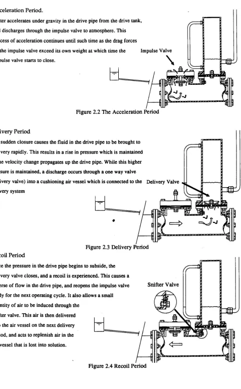
Acceleration Period.

Water accelerates under gravity in the drive pipe from the drive tank,

and discharges through the impulse valve to atmosphere. This

process of acceleration continues until such time as the drag forces

on the impulse valve exceed its own weight at which time the

impulse valve starts to close.

Impulse Valve

H::

Figure 2.2 The Acceleration Period

Delivery Period

The sudden closure causes the fluid in the drive pipe to be brought to

rest very rapidly. This results in a rise in pressure which is maintained

as the velocity change propagates up the drive pipe. While this higher

pressure is maintained, a discharge occurs through a one way valve

\.

(delivery valve) into a cushioning air vessel which is connected to the Delivery Valve

delivery system

Q

_======1

•

Figure 2.3 Delivery Period Recoil Period

Once the pressure in the drive pipe begins to subside, the delivery valve closes, and a recoil is experienced. This causes a

reverse of flow in the drive pipe, and reopens the impulse valve

ready for the next operating cycle. It also allows a small

quantity of air to be induced through the

snifter valve. This air is then delivered

into the air vessel on the next delivery

period, and acts to replenish air in the

air vessel that is lost into solution.

CL

====J

Figure 2.4 Recoil Period

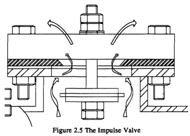
2.2

The Acceleration Period

During this cycle, water accelerates from a source or collection tank, through a length of pipe

known as the drive pipe (see Figure 2.1). This pipe allows the water to fall through a small

distance, accelerating under the force of gravity, and is allowed to discharge at a lower level

through a valve known as the impulse valve.

Figure 2.S1be Impulse Valve

The impulse valve is a simple valve (see Figure 2.5) that is closed by the drag force induced

by a high through flow. The geometry of the valve is such that these drag forces increase

rapidly as the valve moves towards its closed position, so inducing a rapid "snap" closure. See

Figure 2.2.

2.3

Delivery Period

The sudden closure of the impulse valve induces a pressure rise in the drive pipe that is

proportional to the velocity of the fluid in the pipe immediately before the valve closure. This

pressure is maintained while pressure waves propagate along the drive pipe.

During this period in which the drive pipe sustains a high pressure, a small discharge occurs

through a non-return valve (delivery valve) into a vessel containing air at a pressure

approximating to the delivery pressure of the pump. This discharge continues until such time

as the pressure in the drive pipe subsides, at which stage, the non-return valve closes, and the

2.4

Recoil Period

A small remaining velocity in the drive pipe fluid induces a recoil, which in turn induces a

pressure drop at the impulse valve, so allowing it to reopen, and the cyclic operation to recur.

A small air inlet valve (snifter valve) allows a small quantity of air into the drive pipe during

low pressure periods. This is forced through the delivery valve and into the air vessel on the

delivery cycle. This air replaces air that is lost into solution in the air vessel.

The device operates with a cyclic operation of typically 1Hz. The three described phases are

2.5

Detail Function of the Hydraulic Ram Pump

The detailed operation of a hydraulic ram pump as described in the following sections has been determined as a result of a long term study of hydraulic ram pumps involving extensive experimental measurement, computer modelling and simulation.

2.6

Acceleration Period in Detail

The acceleration cycle commences with the opening of the impulse valve. This will usually open under the force of gravity, but is often assisted by the recoil of the previous pumping cycle. The fluid is either stationary, or travelling up the drive pipe towards the feed tank following a velocity recoil in the drive pipe at the end of the previous cycle (this recoil is covered in the following sections).

The fluid in the drive pipe then accelerates under gravity towards the impulse valve. If it is initially in recoil, it decelerates under the differential pressure along the length of the drive pipe imposed by the water level in the drive tank, and this deceleration is increased by friction effects. The equation given in Figure 2.6 gives the deceleration force on the column of fluid in the drive pipe at any instant in time. It should be noted, that this equation assumes the fluid to be a rigid column, and as the wave propagation time is very short compared with

•

the deceleration period, this gives an acceptable approximation for most purposes.

I

~ Ml

l...---J~~==========~

~:celerating

- L

I

M(tJ{ +

M)

A 2dg

Once the fluid is flowing towards the impulse valve, and discharging from it, it accelerates under the action of gravity. This acceleration is reduced by frictional effects.

Time (sees)

Figure 2.8 Velocity History for Acceleration Period

The described acceleration may not be linear because of residual transients propagating in

the drive pipe from the previous pumping cycle as well as changing friction effects. Figure 2.8

illustrates the shape of the velocity history that results from a typical acceleration phase.

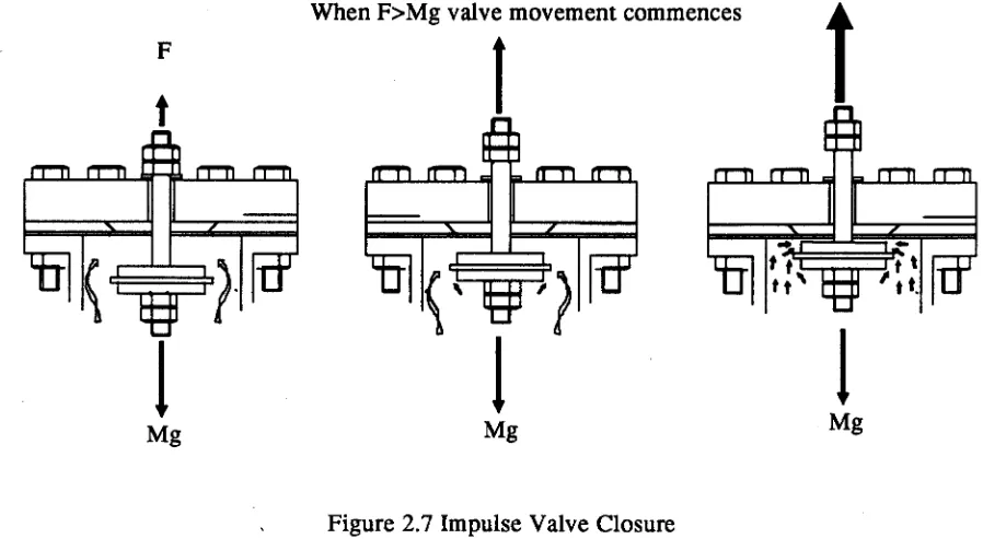
2.7

Valve Closure Period in Detail

The impulse valve disc experiences a drag force as a result of the fluid flowing past it. This

drag force is approximately proportional to the square of the velocity of the fluid flow, and

F

I

t

When F>Mg valve movement commences

t

1

1

1

Mg Mg

proportional to a coefficient of drag for the valve. Once the flow in the drive pipe reaches a level at which the drag force on the valve exceeds the force keeping it open (typically its weight), the impulse valve accelerates towards its closed position.

As the impulse valve disc starts to move, the coefficient of drag increases as the distance

between the valve disc and its seat reduces. Similarly the head loss coefficient across the valve will also increase. This increase in head loss coefficient will act to reduce the acceleration of the flow. The increase in the coefficient of drag will act to increase the acceleration of the impulse valve towards its position of closure.

The valves coefficient of drag increases exponentially as the valve face moves towards the valve seat (this is a characteristic of the type of valve, but is common to the majority of hydraulic ram pumps). This causes an exponentially increasing acceleration on the valve, which in turn leads to a very rapid closure. This valve acceleration is reduced by drag forces restraining the movement of the valve through the fluid in the final stages of closure when the valve velocity exceeds that of the fluid.

The increasing head loss coefficient is significant with respect to the length of the drive pipe, and the acceleration of the fluid. If the drive pipe is relatively short, or the fluid acceleration relatively low, it is possible that the increasing head loss will reduce the velocity of the fluid to such an extent that the drag force on the valve is no longer sufficient to maintain the closure. In this situation, the impulse valve will "bob" up and down, but not reach its seat.

Once the impulse valve reaches its seat, the fluid immediately upstream is brought to a halt.

2.8

Delivery Period in.Detail

The velocity drop and pressure rise propagate upstream in the opposite direction to the

direction of flow. A high pressure wave is also communicated from the three way junction

towards the air vessel. The high pressure wave front will generally reach the delivery valve

well before it reaches the feed tank. The pressure rise experienced is related to the initial

velocity by the equation:

M{=aVo

g - (2.1)

where: I1H = the rise in pressure head (m); a = the velocity of sound in the drive pipe (mls); g

=

=

This is generally referred to as the Joukowsky(4) (1904) pressure head. When this pressure rise reaches the delivery valve, the valve is forced open and fluid is free to flow into the air

vessel. The pressure in the air vessel at this stage is at the delivery head. This flow causes an instantaneous drop in pressure in the main body of the pump. A high frequency pressure

oscillation is induced between the impulse valve and the air vessel water surface on account

of the compressibility of the fluid in the body of the ram.

The opening of the delivery valve causes a new pressure to be sustained. This new pressure

is slightly higher than the pressure in the air vessel on account of the head losses occuring through the delivery valve. The first pressure wave to propagate up the length of the drive

pipe causes a large pressure rise, and brings the' velocity in the drive pipe to a halt. The

opening of the delivery valve causes a second pressure wave to travel up the drive pipe. This

wave front will induce a velocity increase in the drive pipe to allow the delivery flow to

continue, and an associated drop in pressure that is proportional to the increase in velocity.

When the wave front meets the feed tank, the pressure rise is no longer maintained, as there is no inertial change experienced at the reservoir. This effectively transfers a constant head to

the drive pipe. The effect is a wave reflection. The high pressure in the drive pipe is relieved by this pressure wave reflection, and as this wave form propagates back down the drive pipe,

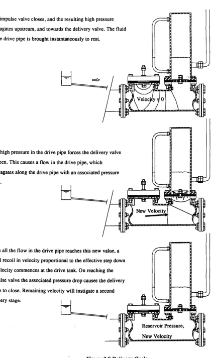
The impulse valve closes, and the resulting high pressure

propagates upstream, and towards the delivery valve. The fluid

in the drive pipe is brought instantaneously to rest.

The high pressure in the drive pipe forces the delivery valve

to open. This causes a flow in the drive pipe, which

propagates along the drive pipe with an associated pressure

drop.

Once all the flow in the drive pipe reaches this new value, a

small recoil in velocity proportional to the effective step down

in velocity commences at the drive tank. On reaching the

impulse valve the associated pressure drop causes the delivery

valve to close. Remaining velocity will instigate a second

delivery stage.

t:i

New Velocity

valve, the magnitude of the relieving pressure becomes smaller because of the friction that

exists in the drive pipe. The pressure that finally arrives at the delivery valve is equal to the

static head supplied by the feed tank, less the friction losses at the new reduced velocity. (See

Figure 2.9).

This new pressure is not sufficient to maintain the delivery pressure, and so the delivery

valve moves towards its dosed position. The nature of the delivery valve is such that there

will be a degree of back flow, and this will vary with operating conditions, but will typically

be equal to the swept volume of the valve. At this stage, the delivery period has undergone its first delivery cycle. There remains a new reduced steady state velocity in the drive pipe.

This velocity effectively meets a closed valve as the delivery valve closes under the

normalised pressures. A pressure rise is induced at the delivery valve that is proportional to

the new velocity in the drive pipe. A new pressure wave then propagates down the drive

pipe, incorporating a Joukowsky pressure rise, and an associated halting of the velocity in the

pipe. This wave propagates up the drive pipe towards the feed tank, but is followed by

another wave front of reduced pressure, and increased velocity associated with the

>.

...

....

g

~

>

Delivery subcycle 1

reopening of the delivery valve.

A typical drive pipe velocity history for the delivery period is given in Figure 2.10. This

illustrates the multiple delivery subcycles. The shaded area represents the volume of water

delivered when multiplied by the drive pipe area.

2.9 Recoil Period in Detail

As before, these waves are reflected at the reservoir, in a normalising pressure wave which

also induces a drop in velocity. When this arrives at the delivery valve, the delivery valve once again closes ( or starts to), and the above cycle recurs. This process of velocity steps

continues until such time as the velocity remaining in the drive pipe is such that the induced

pressure is smaller than the delivery pressure. If this occurs, the whole of the drive pipe becomes pressurised at the new lower pressure and the pressure wave propagates up the

drive pipe. On reaching the reservoir, there is again a reflection involving a reduction in

velocity, and a normalisation of pressure. As the velocity reduction associated with the previous pressure wave travelling up the drive pipe reduced the fluid velocity to zero, this

>.

~

....

o

-

>

Delivery subcycle 1

Delivery subcycle 2

Time

pressure reduction induces a negative velocity known as the recoil. This propagates down the drive pipe towards the delivery valve. This represents an entire wave reflection in which

no deli very occures.

When this negative velocity and pressure normalisation ~rrives at the delivery valve, the delivery valve closes. A negative pressure is then created at the delivery valve, the

downward pressure transient being proportional to the magnitude of the recoil velocity. This

low pressure allows a quantity of air to be induced through a snifter valve located at the

delivery valve. This in turn acts to reduce the magnitude of the drop in pressure, and allows

some of the recoil velocity to be sustained.

When this negative pressure is communicated to the delivery valve, the impulse valve will

typically open under its own weight. If this negative pressure wave is of insufficient magnitude, the valve will fail to reopen. This represents a common reason for pump failure.

This negative velocity pressure wave then proceeds up the full length of the drive pipe. On

reaching the feed reservoir, a reflected wave propagates down the drive pipe normalising the

pressures to reservoir pressure. Small damped pressure oscillations then occur on account of

friction effects. This marks the beginning of the next acceleration cycle.

The velocity history given in Figure 2.11 illustrates the recoil period as described above. This

recoil can be seen to differ from that illustrated in Figure 2.10. In Figure 2.10, the velocity

drop associated with a reflected pressure wave from the reservoir brings the drive pipe

velocity negative which allows the delivery valve to close and the impulse valve to reopen as

above. In this case, there is no residual forward velocity and no additional pressure rise, and

the next cycle can begin immediately. This will marginally increase the frequency, and

therefore the power ouput of the device.

2.10

The Snifter Valve

As mentioned in the above section, the snifter valve operates during the recoil period to allow

a small quantity of air to be induced into the body of the hydraulic ram pump. This will rest

as an air pocket just below the delivery valve. This air will then be transfered to the air vessel

as soon as the delivery valve next opens. The effect of this is to sustain the volume of air in the

Atmospheric

Figure 2.12 The Snifter Valve

There are a number of snifter valve designs used, and the most typical of these is illustrated in Figure 2.12 . It incorporates a simple flap seal over an air inlet orifice. The sizing of this orifice directly influences the volume of air induced on each cycle. It also effects the severity of the negative pressure associated with the recoil, and the magnitude of recoil velocity

attained.

The_orifice is sized empirically to ensure that the quantity of air induced is in excess of that lost into solution. This results in a continuous air discharge into the delivery pipe. This can cause problems downstream, so an air release valve is required immediately downstream of

the air vessel.

2.11 The Significance of this Understanding on Pump Design.

2.11.1 Two modes of recoil effect pump performance.

The observation that there are two ways in which the hydraulic ram pump cycle finishes is

helpful in interpreting sudden frequency shifts in operating pumps and unreliable behaviour

at some delivery heads, and also provides important insight necessary to reliably predict ram

pump performance.

2.11.2 Acceleration efficiency

The concept of acceleration efficiency in this thesis represents the amount of potential energy

The acceleration efficiency in a hydraulic ram pump is closely dependent on the friction experienced in the drive pipe. Similarly, it is also dependent on the acceleration of the fluid

in the drive pipe. This is because with a low acceleration that diminishes significantly with

speed the acceleration period is greatly extended, while the resulting kinetic energy of the

fluid in the pipe is the same for a given final velocity. The result is a significant quantity of

wasted water, and therefore a reduction in pump efficiency and power.

2.11.3 Delivery Efficiency

The concept of delivery efficiency was also invented by the author, and represents the

potential energy attained through the discharge of water to the delivery head as a proportion

of the kinetic energy in the drive pipe at the beginning of the delivery cycle (closure of the

impulse valve).

The efficiency of the delivery cycle has been found to be of some significance. A direct

influence on this is the friction coefficient of the delivery valve. However, other very

significant factors include the swept volume of the delivery valve, and the mode of delivery.

If a hydraulic ram pump incorporates a delivery valve which has a returning force applied to it, the head loss associated with delivery may be much increased, however, the loss of water

as a result of back flow is also greatly reduced. This may compensate for the extra losses

associated with delivery. The significance of this effect increases with higher delivery heads.

2.11.4 High Frequency Oscillations.

The·high frequency oscillations visible in the pressure history given in Figure 2.13, can be

seen to be oscillations between the impulse valve and the air vessel. il, for reasons of

durability, it is necessary to alter the frequency or magnitude of the oscillations, this can be

achieved by dimensional changes within the pump itself. A study of this is illustrated in

chapter 4. A lower frequency oscillation is obtained by increasing the distance between the

impulse valve and the air vessel. The magnitude of the oscillations are reduced by increasing

.

the diameter of the pipework connecting the two. This study was the cause of major changes

60 _--

_'"1---,

..-.

e

' - '

'g

Q)

==

50

40 30

20

10

0

-10

0 _{100 T' ( ) 200}

Ime ms

Figure 2.13 Simulated Pressure Transient in Ram Pump

2.11.S

Snifter Valve Sizing

300

The quantity of air induced into the drive pipe through the snifter valve is quite critical. Too

large a quantity will result in failure of operation of the pump as air will travel up the drive

pipe, and affect the behaviour of the propagating transients. A snifter valve orifice which is

too small will result in insufficient air being induced into the air vessel to replenish that lost

into the delivered water. The result of this will be an empty air vessel, which can potentially

cause significant damage to the pump and delivery pipe work, and will certainly have a

negative effect on performance.

It is evident from the explanation that the quantity of air induced into the drive pipe is also

dependent on the magnitude of the recoil velocity that occurs in the drive pipe. The snifter

valve should therefore be sized or adjusted accordingly.

2.11.6 Time for Valve Closure

From the description of the valve closure period, it is possible to perceive that the major

factor effecting this is the acceleration of the fluid in the drive pipe. As this has a direct effect

on the performance of the pump, it is important that the acceleration of the fluid column is of

a suitably high magnitude when the impulse valve begins to close, to ensure rapid closure of

2.11.7 Impulse Valve Failure To Close

From the description of the delivery valve closure it is possible to understand the interaction

between the impulse valve and the drive pipe during the closure. As the impulse valve

begins to close, the head loss across the valve increases, and this will slow down the fluid in

the drive pipe after a wave reflection time of 2L/ a. A lower velocity will reduce the drag force

on the valve causing it to close, however, the movement of the valve will have increased the

force coefficient for the valve. The net effect is a trade off between an increasing drag

coefficient and a decreasing flow. If the net effect is a force that is less than the weight of the valve, the valve will decelerate. Depending on the severity of the deceleration, and the

velocity of the valve, the valve may never reach its seat, but only ''bob'' up and down.

The above illustrates a problem that is highly dependent on a particular valve's

characteristics. The problem is exacerbated on installations in which the fluid acceleration is

small. Minimum drive pipe lengths and fluid accelerations during the closure cycle should be

quantifiable for a given impulse valve geometry and settings.

2.11.8 Drive Pipe Length

The drive pipe length greatly effects the nature of operation of a hydraulic ram pump.

However, many of the factors that are greatly affected by drive pipe length are cancelling.

For example, a long drive pipe will have a relatively long and inefficient acceleration period,

but will require fewer ram cycles for a given delivery volume. So increased losses associated

with inefficient acceleration are cancelled by reduced losses associated with each valve

closure. For this reason, within a design operating range, the overall performance is largely

unaffected by drive pipe length.

An enhanced understanding of the operation of the hydraulic ram pump enables this

operating range to be more usefully specified.

The acceleration cycle is greatly affected by the length of the drive pipe. The longer the drive

pipe, the more mass that exists to be accelerated by the drive head, and so the slower the

acceleration. Similarly the longer the drive pipe, the more friction that exists on the column of

The valve closure period is affected by the length of the drive pipe. This affects pump performance as a short valve closure period will generally be more efficient. The interaction

between the two is discussed in the above explanation, and more detail is given in Chapter 4

which refers to a study undertaken by the author on this effect using the method of

characteristics simulation.

The delivery cycle is also significantly affected by the length of the drive pipe. The longer the

drive pipe, the longer each of the delivery phases, as each delivery phase lasts a full wave reflection period. A longer delivery phase will deliver proportionately more water.

The recoil period is also directly affected by the length of drive pipe. A recoil on a long drive

pipe will involve more kinetic energy, and will therefore take longer to slow down. This will

reduce the pump beat frequency, and so reduce the output power of the device.

2.12

Summary

This chapter has given a detailed description of the operation of the hydraulic ram pump, and

the interaction of the parameters affecting its performance. Chapter 3 gives a summary of

other analyses undertaken on the hydraulic ram pump, while Chapters 4 and 5 illustrate the

methods employed to obtain and use the described understanding of hydraulic ram pump

Chapter 3:

History of the Hydraulic Ram Pump and Analyses.

The hydraulic ram in its earliest form was invented by John Whithurst of Derby (5) 1772. The

device he created bears little resemblance to the devices of today, and was discovered by chance. He found that a length of pipe that discharged from a reservoir to a low level valve was prone to failure adjacent to the valve. To solve the problem, a small air vessel was connected to the system. This was connected through a one way valve, and a delivery pipework was connected to it. To the surprise of many, water was delivered in this pipe to a level higher than the original source. Unfortunately a continuous delivery was only possible if an individual was deployed to continuously open and close the discharge valve.

Delivery

I

Water Source

Air Vessel

Figure 3.1 The Hydraulic Ram Pump after John Whithurst

A wide variety of hydraulic ram pump devices followed, and hydraulic rams were very

widely deployed, and a large quantity of literature produced before the turn of the century.

Manufacturers also produced dual flow ram pumps capable of pumping clean potable water

using the energy available in falling waste water. Even air compressors were produced that

compressed air by the same operation as a conventional hydraulic ram pump.

3.1

Experimental Research

In the early days of hydraulic ram pumps, extensive experimental work was undertaken on

the device. Documented works include: Eytelwein(7)1805, d' Aubuisson(S)1840, Morin(9)1863,

Tresca(10)1864, Carpenter(11)1894, Richards(12)1898, Church(13)1899, Cia rk(14) 1900,

Anderson(1S)1922 and Clavert(16)1957.

These analyses were invariably based on a single experimental facility and often resulted in

the drawing of sweeping conclusions on hydraulic ram pump design ana operation. A

helpful summary of these is offered by Rennie and Bunt (17)1981. Some of these conclusions

were of significant value in design, but with the lack of theoretical analyses, the conclusions

were often adopted completely regardless of their validity.

3.2

Theoretical Analyses

A number of theoretical analyses of the hydraulic ram pump developed alongside the above

research. Significant works were provided by Montgolfier(6), Venturoli(1S)1818,

Navier(19)1839, Weissbach(20)1897, Rankine(21)1872, Mirapeix(22)1907, Lorenz(23)1910, and

Bergeron(24)1932. None of the above were based on empirical data, and all involved some

erroneous assumptions. A summary of these is also available in the work by Rennie and

Bunt(17).

The above analyses differed in the sophistication with the pumping cycle being subdivided

to varying degrees, from two divisions in the theory proposed by Navier to typically four

divisions adopted by the majority to represent a range of different theoretical periods.

Although the above theories offered a wider perspective than the purely empirical studies,

errors in assumptions and the crudeness of the analyses severely hampered their usefulness.

An attempt to combine experimental data with theoretical analyses was first undertaken by

but he was able to confirm a correlation between experimental and theoretical behaviour

during the acceleration period.

As measurement technologies became more sophisticated, the understanding of the transient

behaviour in the hydraulic ram pump developed. In the 1930's O'Brien and Gosline(26) using the research undertaken by Harza (25), provided a theoretical and experimental investigation

into hydraulic ram pumps which in retrospect was inspired. They provided a theoretical

analysis of the transient behaviour in the drive pipe during the delivery cycle. The simulation

work undertaken in this study largely verifies the analysis proposed. Unfortunately many

subsequent analysis did not acknowledge or adopt the development attained, and later work

by Krol(27)1947 provided a detailed analysis that was widely adopted, but failed to

incorporate the work of O'Brien and Gosline.

A brief summary of the analytical results obtained by O'Brien and Gosline is given in the following section. Beyond this analysis, there were attempts to utilise the graphical method

of transient analysis for which Schyder(28)1932 and Bergeron(24) are famed. The work of Krol

has been adopted by a number of more recent studies.

3.3 Summary of more recent Analyses of the Hydraulic Ram Pump

3.3.1

O'Brien and Gosline(26)1933

A diagrammatic summary of O'Brien and Gosline's theoretical analysis of the hydraulic ram

pump given in Figure 3.2 shows that the researchers were able to predict the characteristic

behaviour identified by the simulation developed within this research. In this respect, their

research is unique, and unfortunately largely unrecognised except within the work of Rennie

and Bunt. The analysis offered for much of the hydraulic ram cycle was typical of such

analyses, but their analysis of the delivery cycle was unique, and they were able to predict the

intricacies of the delivery cycle that are modelled in detail in chapter 5 of this thesis.

O'Brien and Gosline avoid providing a prediction of overall efficiency on the grounds that

such a calculation would be excessively complex. However, they do offer an expression for

acceleration efficiency. This is a valuable concept, and is covered in the proposed design charts in Chapter 6. The reason given for this is that acceleration efficiency dominates in

but is, however, fundamentally flawed, as other inefficiencies such as poor valve closure times can rapidly dominate.

e

=

en en

e

Il..

Drive Head

~~--====~---+---

8-it

Q)

>

·c

s::

....

Delivered Volume

Wasted Volume '

Time

Figure 3.2 Representation after O'Brien & Gosline

3.3.2 Krol(27)1947

A very detailed analysis was provided by Krol using calibrated data from a hydraulic ram pump. It is interesting to note Krol's use of friction and head loss coefficients to determine closure times and flows. It is also interesting to note the degree of success he attained with these. The major failings of his analysis were as a result of his denial of the transient wave propagation during the delivery cycle. His modelling of the impulse valve was valuable, but limited in that it assumed constant drag coefficients. It is possible to see from the calibrations undertaken in chapter 4 that this is clearly an unacceptable assumption.

3.3.3

Rennie and

1981

)

Krol, they adopted the graphical method(24) to solve the behaviour of the impulse valve during closure and the transient regime that followed. In spite of the difficulty involved with representing complex transients using the graphical method, useful results were obtained.

3.3.4 Yau-Chung Chiang(29)

1984

University of Wisconsin-Madison

This was an interesting study into simulation and optimisation of transient oscUlation flow and sound in complex piping systems. The study utilised the hydraulic ram pump as a case study, and created a crude "method of characteristics" simulation of the device, and then proceeded to apply the optimisation routines to the device. The study suffered considerably as a result of the crudeness of the hydraulic ram model adopted. Further problems found were similar to those described in chapter 4, where the quantity of data and variables existing in a single simulation are so great that attempts at optimisation are severely hampered. Chiang attempted to overcome this by considering aspects of design in isolation. This was a valuable approach, but the results obtained suggested improvements in efficiencies to levels far below those currently attained.

3.4

Summary

It is clear that there has been significant research into the hydraulic ram pump, and much of it highly replicatory. The reason for this is largely due to the massive complexity of interacting variables that are involved in an apparently very simple phenomenon. Poor results in much of the early work were a result of poor measurement technologies.

It is interesting to note that as the measurement technologies improved so did the theoretical analyses. The theoretical success of O'Brien and Gosline seemed to be closely related to their ability to measure transient pressures. The work of Krol some years later however, failed to achieve the insight offered by O'Brien and Gosline.

Rennie and Bunt where able to progress Krol's understanding with an improved understanding of hydraulic transients, although the methods used to analyse these are somewhat antiquated, and not without their inadequacies.

Chapter 4:

Computer Simulation of the Hydraulic Ram Pump

4.1

Summary of simulation

An important tool in the analysis of the hydraulic ram pump was a computer simulation of

the device. The development of the simulation was initiated during the author's MSc

research. This simulation utilised the extensively documented "method of characteristics" to

solve the partial differential equations of motion and continuity together with standard

algorithms for the modelling of boundary conditions for the reservoir and air vessel present

in a hydraulic ram. Some innovation was required with respect to modelling some of the

more dynamic boundary elements.

4.2

The modelling of pressure transients in a pipe

A method of characteristics simulation enables an accurate modelling of pressure transients

in a pipe. Although developed during the 1950's the method was popularised by Victor

Streeter and Ben Wylie(30)1993 of the University of Michigan. The majority of modem

transient simulation work currently undertaken utilises this explicit finite difference method

known as the "method of characteristics". The equations used to determine transient flows

and pressures in a pipe using a fixed time step are given in Appendix B.

Recent attempts have been made to employ finite element techniques for transient analysis,

but these have involved severe limitations (Watt and Boldy(31» . The decision to use a

method of characteristics simulation was made for the following reasons:

• The finite element methods available are not readily suited to sharp wave front

transients of the type induced in a hydraulic ram pump.

• The use of finite element techniques for complex pipe systems involves the

production of some highly sophisticated shape functions which although quick

to solve, do not allow minor modifications at a later stage.

• It was anticipated that drastic modification to both program structure and boundary conditions would be carried out in an evolutionary manner. Such

modifications are well suited to a "method of characteristics" simulation as it

effecting the integrity of the rest of the simulation.

• The "method of characteristics" is used widely in the simulation of hydraulic

transients in water pumping systems, and much research has been published

on the most accurate means to represent various commonly occurring

boundary conditions. Streeter and Wylie(30),Chaudry(32),Fox(33) ,5waffield and

Boldy(34), Thorley(35).

The "method of characteristics" requires a good estimate for the transient wave propagation

velocity for each pipe section. To determine this, Joukowsky(4)(1898) and Gibson(36)(1908)

developed a concept of a 'Virtual Bulk Modulus of Elasticity" which also accounts for the

pipe materials and dimensions. Joukowsky's calculation assumed. a linear constraint on the

pipe, and so has become the more widely adopted solution. This led to the following equation for pressure wave propagation velocity of:

-;::::===1

=:;:==-a - .

- " p

[1.

+

K tE

where:

a

=

p

₌

(4.1)

K

₌

D

=

=

E

₌

means by which the pipe is restrained:

For pipes restrained at one end only :CI

=

~

For pipes anchored throughout their length: Cl

=

For pipes with expansion joints along their entire length: Cl

=

Equation (4.1) has been used extensively in this study to predict the speed of pressure wave propagation. The wave speed propagation time was also monitored using sequentially placed pressure transducers which were sampled using a 500kHz analogue to digital converter. This system was used to verify the calculated pressure wave propagation speeds as well as experimentally monitor pressure transients in pipelines.

4.3

The Reservoir Boundary

Submersible Pump

Counesy 01 KSB

Figure 4.1 Experimental Rig

The reservoir boundary condition used is a standard boundary condition used for transient simulation. The equation that describes the boundary condition for outflowing water is simply

v

Hx = Reservoir Level - 2g (4.2)

where Hx is the pressure at the exit from the reservoir; V is the exit velocity, and g is the acceleration due to gravity.

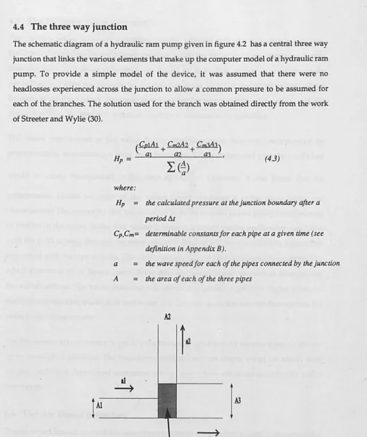
4.4

The three way junction

The schematic diagram of a hydraulic ram pump given in figure 4.2 has a central three way

junction that links the various elements that make up the computer model of a hydraulic ram

pump. To provide a simple model of the device, it was assumed that there were no

headlosses experienced across the junction to allow a common pressure to be assumed for

each of the branches. The solution used for the branch was obtained directly from the work

of Streeter and Wylie (30).

(4.3)

where:

Hp

=

Cp,Cm

=

definition in Appendix B).

a = the wave speedjor each oj the pipes connected by the junction

A

=

A2

!M

- - -

l~

13)

4.5

The Delivery Valve Boundary

The delivery valve boundary condition initially adopted was one of a simple two way

junction with a facility for a diameter variation across the valve, and a mechanism to ensure

that any backward flows calculated are forced to zero. This represents a highly crude

modelling as it does not account for friction across the valve, or the swept volume of the

delivery valve. No attempt was made to account for the swept volume of the valve until the

model described in chapter 5 included a facility to account for its operation.

The losses experienced at the valve during discharge were, however, incorporated by

experimentally determining a head loss coefficient. It was anticipated that the coefficient

would be easily incorporated in the form Hf=

Ct

~

.

characteristic. The reason for this was believed to be on account of two parallel' mechanisms

of friction in the valve. In the first instance, there is a simple orifice mechanism associated

with the fluid passing through the valve orifice(s). Beyond this there is a friction mechanism

associated with the type of valve. The most common type of valve incorporates a rubber disc,

which distorts to allow flow through in the delivery direction, and recovers its shape to seal

the valves orifices. The valve, therefore will distort to a greater degree for higher flows, so

significantly reducing the friction coefficient. It is this part of the mechanism that explains the

more linear characteristic.

For this reason, it is necessary to modify the boundary condition for various typesof delivery valve boundary conditions. The boundary condition can then simply adopt the steady state

friction coefficient determined experimentally for every flow condition experienced under

simulation.

4.6

The Air Vessel Boundary

The air vessel boundary condition incorporated into the simulation is used to determine the

quantity of fluid delivered per pumping cycle and the continuous delivery flow rate. The