Set up for assessment of localisation accuracy of Structure from Motion algorithms

Set-up for reproducible, conditioned experiments

related to 3D surface reconstruction from

image sequences

A.G. (Alexander) Green

BSc Report

C

e

Dr.ir. F. van der Heijden

Prof.dr.ir. R.N.J. Veldhuis

Dr. F.J. Siepel

June 2017

012RAM2017

Robotics and Mechatronics

EE-Math-CS

University of Twente

Set-up for assessment of localisation accuracy of

Structure from Motion algorithms

Alexander G. Green – [email protected] – s1012789

May 25, 2017

Abstract—This paper discusses the need for a reliable experi-mental set-up providing a consistent benchmark to facilitate the assessment of the accuracy of localisation in varying implemen-tations of Structure from Motion algorithms. The physical set-up involves a KUKA LWR4+ arm robot and a USB camera, both connected to a personal computer.

A key step in determining the trajectory of the camera is finding its pose relative the robot arm’s end effector. Two methods are introduced in this paper to address this problem. These methods are subjected to simulated and real-world tests. One method clearly outperforms the other when dealing with noisy, real-world extrinsic camera calibration at the cost of vastly increased computational complexity.

I. INTRODUCTION

R

ELIABLE camera localisation is vital for many applica-tions regarding spatial measurements and presentation. One such application is 3D surface reconstruction from 2D image data. This can be achieved through range imaging techniques which apply triangulation to feature points matched in image frames taken by cameras positioned at different loca-tions. Similar to the stereopsis that most of us enjoy, a stereo camera uses two lenses with a known transformation between each other in order to acquire a sense of depth. However, reconstructing a 3D surface from just two narrow vantage points often does not suffice. An increase in the number of vantage points can be attained by employing multiple cameras. This requires knowing their translation and orientation (pose) relative to each other, or by moving the camera and accurately tracking the motion (often referred to asStructure from Motion

or SfM), which is where reliable camera localisation comes into play.

The increasingly prevalent field ofaugmented reality (AR) also relies heavily on accurate camera localisation to correctly augment the image feed with visual aids depending on the vantage point. Medical applications of AR often involve endoscopic biopsies in which biopsy sites are tracked and projected onto the image plane “facilitating re-targeting and serial examination” [1]. Keeping track of which segments have been examined can be difficult without proper localisation. This can lead to incomplete examinations which in turn increases the miss rate for pathological conditions [2]. Another medical application of AR can be employed in brain tumour resection [3]. Planning surgery of this nature can involve the use of neuronavigational systems which reconstruct a 3D visualisation through MRI images. After the optimal surgical pathway has been determined it can be projected onto the

live video feed, aiding the surgeon’s navigation in this most precarious endeavour.

In many practical applications the camera is not fastened to a robot’s manipulator. If no other reliable data regarding the camera’s pose at the time of the image frames is available, one must resort to visual localisation. The use of artificial features (fiducials) can drastically simplify the camera resectioning problem. The application of such features, however, can be impractical or even impossible in certain circumstances such as endoscopic biopsies. Development of algorithms addressing this localisation problem require reproducible and conditioned experiments. A reliable experimental set-up can provide a con-sistent benchmark to facilitate the assessment of the accuracy of localisation in varying implementations of SfM. To provide a consistent benchmark, the camera’s pose should be available in a constant coordinate frame, regardless of changes in camera model or mounting method between runs.

This paper presents an experimental set-up and calibration algorithms to accurately localise the camera relative to a robot arm’s end effector. Since the robot arm can be precisely tracked through forward kinematics, the camera can be tracked with the accuracy of the calibrated, static transformation between the manipulator and the camera, without suffering from drift. Comparing the trajectory found through this method with the trajectory of an SfM method provides insight into the accuracy of this implementation. The main research question is how to obtain the camera’s pose relative to a robot’s end effector.

Consistency relies on accurately measuring the pose of the camera relative to the arm’s manipulator. This process will be referred to ashand-eye calibration. It is vital in several aspects including the following [4].

• An automated 3D robotics vision measurement of the

spatial relationships between points on an object can be done by moving the camera to different positions in the workspace. The poses of the camera must be known in order to relate the images to each other. If the robot system is capable of computing its manipulator’s pose and the camera is rigidly fastened to this manipulator, the pose of the camera in the robot coordinate frame can be computed through hand-eye calibration.

• The aforementioned automated 3D robotics vision

the transformation between manipulator and camera to be known.

The physical set-up will consist of an arm robot, a monoc-ular camera, a fiducial marker, and a personal computer. A software package will be provided to control the arm, calibrate the camera’s intrinsics, and compute the camera’s trajectories. The desired accuracy of the camera localisation has a maximum translation error of 0.1 mm and rotation error of 0.1 degree.

The following sections will provide an abstract overview of the calibration problem and will be followed by a discussion of the practical implementation of the procedure. A series of tests are performed to evaluate the efficacy of the system. The results of these tests are presented and will be followed by an interpretation thereof, leading to recommendations for further development.

II. MATERIALS

The set-up is realised with the following hardware.

• KUKA LWR4+arm robot with an absolute unidirectional

accuracy of 1.0 mm [5].

• Logitech C270USB camera with a resolution of 720p.

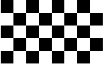
• Calibration marker as shown in Figure 1 with a square

size of 30 mm.

• Personal computer connected to the robot through an

[image:3.595.374.483.59.133.2]

ethernet cable and to the camera through USB The software used is detailed in Section IV-B.

Figure 1: Calibration marker consisting of an asymmetric square pattern

III. CALIBRATION PROBLEM

In order to localise the camera, its extrinsic parameters (pose) need to be computed relative to the robot’s base, which will be referred to as the reference frame. This calibration problem consists of the following coordinate frames.

• Camera{C}

• Calibration marker{M} • Flange{F}

• Reference frame{R}

The coordinate frames and their relative poses are repre-sented graphically as a directed graph in Figure 2.

Of interest is the pose of the camera relative to the flange to which it is rigidly fastened. This transformation (FTC) can

be computed by comparing their respective trajectories.

M C(n)

R F(n)

R_T F(n) R

TM

RTC

(n) FTC C_T

[image:3.595.77.258.404.515.2]

M(n)

Figure 2: Directed graph of the coordinate frames and their relative poses

The pose data of the flange !RTF

"

is provided by the KUKA System Software, calculated through forward kinemat-ics based on its seven joints. The trajectory of the camera can be extracted from image frames containing a calibration marker. The poses received through this visual localisation method are defined in the coordinate system of the marker.

The following sections will discuss two methods developed for computingFTC.

A. Bipartite method

The method for determining the transformation between the flange and the camera !F_T

C

"

is divided into an orientation part !F_R

C

"

and a translation part !F_t C

"

, which require a trajectory consisting of pure translations and pure rotations respectively.

1) Orientation: The camera’s trajectory is considered from timeiandjas a displacement relative to its coordinate system at timei{Ci}(see Figure 3). One can derive the displacement

as follows.

M

T−1

C (i) M

TC(j) =CTM(i)MTC(j) =CiTCj (1)

=Ci_R

Cj

Ci_t

Cj =

Ci_t

Cj (2)

Here R and t are a transformation matrix and a translation vector, respectively. Equation (2) follows from the fact that the trajectory has no rotation !Ci_R

Cj =I

"

. This can be applied to the trajectory of the flange as well:

R

T−1

F (i) R

TF(j) =FTR(i)RTF(j) =FiTFj (3)

=Fi_R

Fj

Fi_t

Fj =

Fi_t

Fj (4)

{ }

F

_i

{ }

F

_j

{ }

C

_i

{ }

C

_j

θ

FC

v

_C

v

_F

[image:3.595.336.548.525.715.2]

In the two dimensional case, the angle (θF C)between the

two displacements(vF andvC)can be obtained by

normalis-ing them and applynormalis-ing the inverse cosine to their dot product:

θF C = cos−

1

#

vF

∥vF∥

· vC

∥vC∥

$

(5)

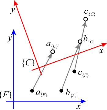
Comparing at least three noncollinear points with equal ori-entation within both {C} and {F} will give the orientation between the camera and the flange (see Figure 4). The rotation between two coordinate frames can be obtained by applying the Kabsch algorithm [6]. This is a procedure for computing the optimal rotation between two given vector sets.

x

y

{ }

F

a

{ }F

b

{ }F

c

{ }F

x

y

{ }

C

a

{ }C

b

{ }C

[image:4.595.341.516.55.245.2]

c

{ }C

Figure 4: Relating two points is enough to compute the orientation between two 2D coordinate frames, a third is needed when relating 3D systems.

2) Translation: A rotation around an axis gives the distance from that axis. This forms a cylinder of possible solutions. A rotation around two axes gives the intersection of two cylinders and so on. While three cylinders gives eight points (see Figure 5), four can be excluded for lying in the negative

z volume. To narrow it down to a single point, knowing in which quadrant of the xy plane of the flange it falls would suffice, as would adding two more rotation axes.

The algorithm to determine these points is explained in the following steps.

1) Perform three rotational trajectories with orthogonal axes of rotation.

2) For each trajectory findCi_TC j and

Fi_TF j.

3) Find the rotation axis of each Fi_TF

j by solving

Fi_TF

jα=α. This real eigenvector forms the direction

of one cylinder.

4) Determine the Euclidian norm (d) of the distance tra-versed by the camera relative to the flange:

d=∥Ci_T

Cj∥ − ∥

Fi_T

Fj∥ (6)

5) Determine the radius (r) of the cylinder:

r= d

2 sin!α

2

" (7)

y

[image:4.595.79.254.221.402.2]

x

z

Figure 5: Knowing the distance from three axes gives eight possible translation vectors. This image was generated with a translation vector at(3,4,5).

6) The radius of a cylinder can be related to the position of the potential points along the orthogonal axes:

r2a=b

2

+c2 r2b =a

2

+c2 r2

c =a

2

+c2

The locations can be resolved and aligned to Cartesian axes:

pa=aαa=±

%

r2

b+r

2

c−r

2

a

2 αa (8)

pb=bαb=±

%

r2

a+r

2

c −r

2

b

2 αb (9)

pc=cαc=±

%

r2

a+r

2

b −r

2

c

2 αc (10) 7) Summing the contributions of each axis will results in a potentialFtC. Since each axis grants two possibilities,

there are23

= 8potentialFtC.

B. Procrustes method

This method tries to approach the optimal transformation through iteratively applying the Procrustes method. The algo-rithm to findFTC is explained in the following steps.

Known:R_T

F(n)andMTC(n), forn= 0,1, . . . , N. IfFtC

were to be known, then: 1) RtC(n) =RTF(n)FtC

2) MtC(n)is known fromMTC(n).

3) Apply Procrustes to computeMTRfrom steps 1 and 2.

4) Calculate the goodness of fit:

J = 1

N

N

&

n=1 ∥M_t

C(n)−MTRRtC(n)∥

2

J is dependent on FtC. If FtC was correct, then

J!F_t C

"

5) Ft'C =argmin J

!F_t C

"

6) Apply Procrustes again to computeMTRwith the newly

foundF_t' C.

7) CalculateM_t

F(n) =MTRRtF(n).

8) Apply Procrustes yet again to compute F_T C from M_t

F(n)andMtC(n).

C. Tsai-Lenz method

The following method is adopted from a paper from Tsai and Lenz [7].

To compute the orientation of the camera relative to the flange, we first compute the time derivative of the rotation axis

!_C

r′

F

"

from the rotation axis describing the rotation between timeiandj for both the camera and the flange.

Skew(Fi_r′

Fj+

Ci_r′

Cj

)

C

r′

F = Fi_r

Fj +

Ci_r

Cj (11)

The skew-symmetric matrix of a vector v is generated as follows.

Skew(v) =

⎡

⎣ 0 −vz

vy

vz 0 −vx

−vy vx 0

⎤

⎦ (12)

FindingCr′

F leads us to the rotation angleθF C and rotation

vectorCrF.

θF C = 2 tan−

1

|C_r′

F| (14) C

rF =

2C_r′

F

.

1 +|C_r′

F|

2 (15)

The rotation matrix !FRC

"

can be computed from the rotation angle and axis through Equation (13) on p. 5. Once the orientation is known, the transformation can be computed, provided one has at least two sets ofi andj, by solving the following linear system of three linear equations withFTC as

unknowns.

!Fi_R

Fj −I

"F

TC =CRFCiTCj−

Fi_T

Fj (16)

IV. PROCEDURE

The calibration system can be compartmentalised into sev-eral modular components. These components can be seen in the functional structure of the process depicted in Figure 6. The functionality of these components and their software implementation are described in this subsection.

A. Functionality

In order to assign physical dimensions through planar homography and to negate the disturbance caused by lens distortion one must perform intrinsic calibration. This can be achieved by having a camera observe a planar pattern from several, different orientations [8].

Once the camera is calibrated, the distance a point travels in the image plane relative to the distance the camera moved (motion parallax[9]) will provide us with enough information to compute the distance between that point and the focal point. Combining this information with the angle from the principal

axis based on the pixel coordinates, results in the position of the point being computable in the camera’s coordinate system. The pose of the flange can be determined through kinematic equations based on the state of the joints [10]:

F =A1A2E1A3A4A5A6 (17)

In our case the arm has seven joints, each with one degree of freedom (DoF). Therefore, the arm has seven degrees of freedom, meaning it can assume any position and orientation within its workspace while being able to afford to lose a DoF when encountering a singularity and continue its trajectory without discontinuities.

B. Software implementation

The software implementation is built using the Robot Op-erating System (ROS) middleware as a framework to collect the sensor data (raw camera images and joint angles) and MATLABto process the data.

1) Image frames: The raw image frames of the camera are obtained through the ROS packageusb_cam1_.

2) Intrinsic camera calibration: The intrin-sics of the camera are computed with the

estimateCameraParameters2function from MATLAB’s Computer Vision System Toolbox.

3) Marker tracking: The camera’s pose relative to a calibra-tion marker can be found through theextrinsics3function from MATLAB’s Computer Vision System Toolbox.

4) Arm positioning: The arm can be moved manually through the KUKA Control Panel or through commands sent through the Fast Research Interface4 _(FRI).

5) Forward kinematics: Whichever method is used to move the arm, an FRI instance must be running to be able to read the joint angles. These angles are used to compute the pose of the flange with the fkfunction (see Appendix B-A).

6) Hand-eye calibration: The three hand-eye calibration methods described in III-A each have their separate imple-mentation.

a) Bipartite method: This method contains separate methods for finding the orientation and the translation of the camera relative to the flange. The orientation part relies on the procrustes5 function from MATLAB’s Statistics and Machine Learning Toolbox for finding the optimal rotation between the trajectory of the camera and the flange. An imple-mentation can be seen in Appendix B-B. An impleimple-mentation of the cylinder method relies only on standard trigonometric functions as can be seen in Appendix B-C.

b) Procrustes method: This method relies heavily on the

procrustesfunction mentioned above. An implementation can be seen in Appendix B-D.

c) Tsai-Lenz method: For this method a MATLAB im-plementation can be found on Zoran Lazarevic’s homepage6

1_{http://wiki.ros.org/usb cam}

2_{http://nl.mathworks.com/help/vision/ref/estimatecameraparameters. html} 3_{https://nl.mathworks.com/help/vision/ref/extrinsics.html}

4_{http://cs.stanford.edu/people/tkr/fri/html/}

5_{https://nl.mathworks.com/help/stats/procrustes.html}

6_{http://lazax.com/www.cs.columbia.edu/∼laza/html/Stewart/matlab/}

R=

⎡

⎣ cos

θ+r2

x(1−cosθ) rxry(1−cosθ)−rzsinθ rxrz(1−cosθ) +rysinθ

ryrx(1−cosθ) +rzsinθ cosθ+r

2

y(1−cosθ) ryrz(1−cosθ)−rxsinθ

rzrx(1−cosθ)−rysinθ rzry(1−cosθ) +rxsinθ cosθ+rz2(1−cosθ)

⎤

⎦ (13)

Intrinsic calibration

Marker tracking

Hand-eye calibration

Arm positioning

Forward kinematics

[image:6.595.99.232.120.252.2]

Camera in robot frame

Figure 6: Functional structure of the process

7) Camera in robot frame: After the full transformation between flange and camera is computed, placing the camera in the robot coordinate frame (world coordinates) is as trivial as applying this transformation to the flange transformation in the robot coordinate frame found throughfk. To help visualise these transformations, the functioncfplot was written (see Appendix B-G).

V. RESULTS

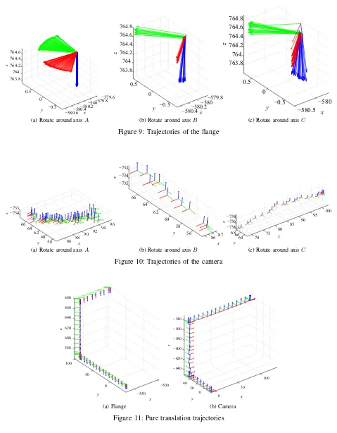
Test trajectories were run to assess the accuracy of the calibration algorithms discussed in Section III. All methods use the pure rotation trajectories as seen in Figure 9 in Ap-pendix A. The bipartite method also requires a pure translation trajectory as seen in Figure 11.

The same flange data is used for both the simulation and the real-world test. The simulation, however, involves a predetermined, randomF_T

C andMTR from whichMTC(n)

is computed. The real-world test on the other hand employs actual extrinsic camera calibration to computeM_T

C(n).

A. Simulation

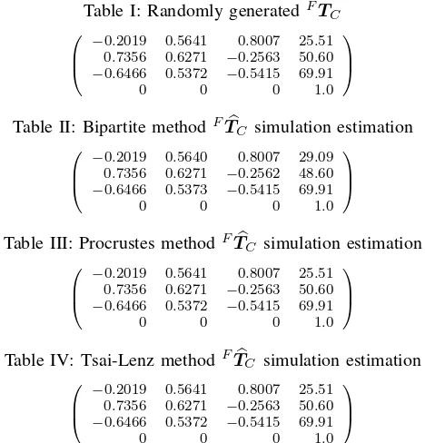
The simulation involves a predeterminedFTC(see Table I)

to facilitate the comparison of estimated and actual values.

1) Bipartite method: The bipartite method uses the pure translation trajectory to compute the orientation of the camera relative to the flange and the pure rotation trajectory is used to compute the translation. Combining these results gives us the estimated flange-to-camera transform

(

F_T' C

)

as seen in Table II.

2) Procrustes method:The Procrustes method only requires the pure rotation trajectory. The estimated flange-to-camera transform

(

F_'

TC

)

can be seen in Table III.

3) Tsai-Lenz method: The Tsai-Lenz method also only requires the pure rotation trajectory. The estimated flange-to-camera transform(F_T'

C

)

can be seen in Table IV.

For clarity, the predetermined transformation and the es-timations are combined in Figure 7. The errors of each estimation can be found in Table V.

25.5 26 26.5 27 27.5 28 28.5 29 29.5

x[mm] 48.5

49 49.5

50 50.5

51

y

[mm]

Figure 7: Predetermined, randomF_T

C and the Procrustes and

Tsai-Lenz estimations overlap on the left. The bipartite method estimation can be seen on the right. The z-axis was omitted for spacial clarity.

B. Real-world test

For the real-world test, we employ extrinsic calibration to attain the pose of the camera relative to the marker. The trajec-tories of the flange and the camera can be seen in Appendix A in Figure 9 and Figure 10, respectively. The estimated values of the pose of the camera relative to the flange can be found in Tables VI, VII, and VIII. A plot of these transformations can be seen in Figure 8. The differences between the results of the methods are summarised in Table IX.

12.5

x

[mm]

−

6

.0

−

5.8

−

5.6

−

5.4

−

5.2

−

5

.0

−

4.8

−

4.6

−

4.4

−

4.2

−

4

.0

y

[mm]

a

b

c

[image:6.595.313.534.148.297.2]

13.0

1 5

3.

Figure 8: FTC computed with three methods: a Bipartite,

[image:6.595.336.518.502.705.2]

[image:7.595.49.283.73.317.2]

Table I: Randomly generatedFTC

⎛

⎜ ⎝

−0.2019 0.5641 0.8007 25.51 0.7356 0.6271 −0.2563 50.60

−0.6466 0.5372 −0.5415 69.91

0 0 0 1.0

⎞

⎟ ⎠

Table II: Bipartite methodFT'C simulation estimation

⎛

⎜ ⎝

−0.2019 0.5640 0.8007 29.09 0.7356 0.6271 −0.2562 48.60

−0.6466 0.5373 −0.5415 69.91

0 0 0 1.0

⎞

⎟ ⎠

Table III: Procrustes methodF_T'

C simulation estimation

⎛

⎜ ⎝

−0.2019 0.5641 0.8007 25.51 0.7356 0.6271 −0.2563 50.60

−0.6466 0.5372 −0.5415 69.91

0 0 0 1.0

⎞

⎟ ⎠

Table IV: Tsai-Lenz methodF_T'

C simulation estimation

⎛

⎜ ⎝

−0.2019 0.5641 0.8007 25.51 0.7356 0.6271 −0.2563 50.60

−0.6466 0.5372 −0.5415 69.91

0 0 0 1.0

⎞

⎟ ⎠

Table V: Error metrics of the simulation results shown as the summation of the Euler angle differences and the norm of the translation differences to the generatedFTC

Angle [degrees] Translation [mm] Bipartite 4.4×10−3 _4.1

[image:7.595.47.279.363.639.2]

Procrustes 2.2×10−5 8.6×10−5 Tsai-Lenz 3.1×10−13 4.4×10−13

Table VI: Bipartite methodFT'C reality estimation

⎛

⎜ ⎝

0.7156 0.6966 0.0510 12.06

−0.6957 0.7174 −0.0370 −5.39

−0.0624 −0.0090 0.9980 74.61

0 0 0 1.0

⎞

⎟ ⎠

Table VII: Procrustes methodFT'C reality estimation

⎛

⎜ ⎝

0.7478 0.6565 0.0987 12.63

−0.6599 0.7513 0.00255 −4.65

−0.0725 −0.0670 0.9951 74.23

0 0 0 1.0

⎞

⎟ ⎠

Table VIII: Tsai-Lenz method FT'C reality estimation

⎛

⎜ ⎝

0.6974 0.7165 0.0138 13.07

−0.7167 0.6972 0.0167 −5.06 0.0023 −0.0216 0.9998 74.58

0 0 0 1.0

⎞

⎟ ⎠

Table IX: Error metrics of the real-world test results shown as the summation of the Euler angle differences and the norm of the translation differences between estimations

Angle [degrees] Translation [mm] Bipartite↔_{Procrustes 6.8 1.0040}

Bipartite↔_{Tsai-Lenz 5.9 1.0627}

Procrustes↔_{Tsai-Lenz 11.6 0.6996}

VI. DISCUSSION

Based on the simulation results, it can be said that all three algorithms can accurately estimate the orientation of the camera relative to the flange. Estimating the translation however, poses a problem for the bipartite method in both the x andy axes. The limited angles of the flange trajectory can be the cause of the discrepancy; whereas the flange can freely roll while keeping the calibration marker in frame, only a slight tilt and yaw is allowed. This limits the accuracy of the cylinder radii estimation. As can be noted from Figure 5, a slight variation in radius can have significant influence on the intersection point coordinates.

The results from the real-world test again show the bipartite method’s translation estimation deviates significantly more along thexandyaxes. While thezvalue merely varies with a range of less than a quarter of a millimetre between methods, the accuracy of these estimations is disputable; all methods base their estimations on the same extrinsic camera calibration data which is by far the least accurate along this axis. A small deviation in perceived marker size has major consequences for the distance estimation compared to an erroneous perceived translation parallel to the calibration marker plane. This error could be reduced by decreasing the distance between the marker and the flange. This will, however, further limit the tilt and yaw angles for keeping the marker in frame. Besides, this distance should approach the camera’s focal distance.

The tilt and yaw limits reveal a strict limit provided by the chosen rotational trajectories. Having the flange move along an arc over the marker (instead of rotating with a static position) would greatly increase the viewing angles while allowing closer proximity to the marker at the expense of increased kinematic planning complexity.

REFERENCES

[1] P. Mountney, S. Giannarou, D. Elson, and G.-Z. Yang,Optical Biopsy Mapping for Minimally Invasive Cancer Screening, pp. 483–490. Berlin, Heidelberg: Springer Berlin Heidelberg, 2009.

[2] H. A. Shah, L. F. Paszat, R. Saskin, T. A. Stukel, and L. Rabeneck, “Factors associated with incomplete colonoscopy: A population-based study,” inGastroenterology, pp. 2297–2303 vol.132, Mar 2007. [3] K. Abhari, J. S. H. Baxter, E. S. Chen, A. R. Khan, C. Wedlake, T. Peters,

R. Eagleson, and S. de Ribaupierre, The Role of Augmented Reality in Training the Planning of Brain Tumor Resubsection, pp. 241–248. Berlin, Heidelberg: Springer Berlin Heidelberg, 2013.

[4] R. Y. Tsai and R. K. Lenz, “Real time versatile robotics hand/eye calibration using 3D machine vision,” in Proceedings. 1988 IEEE International Conference on Robotics and Automation, pp. 554–561 vol.1, Apr 1988.

[5] F. Geiselhart, “Accuracy of KUKA Robot: LBR 4.” Customer sheet designed 3 Mar 2006.

[6] W. Kabsch, “A solution for the best rotation to relate two sets of vectors,” Acta Crystallographica subsection A, vol. 32, pp. 922–923, Sep 1976. [7] R. Y. Tsai and R. K. Lenz, “A new technique for fully autonomous

and efficient 3d robotics hand/eye calibration,” inIEEE Transactions on Robotics and Automation, vol. 5, pp. 345–358, 1989.

[8] Z. Zhang, “A flexible new technique for camera calibration,” IEEE Transactions on Pattern Analysis and Machine Intelligence, vol. 22, pp. 1330–1334, Nov 2000.

[9] R. I. Hartley and A. Zisserman,Multiple View Geometry in Computer Vision. Cambridge University Press, ISBN: 0521540518, second ed., 2004.

APPENDIXA TRAJECTORY PLOTS

763.8 764 764.2

z

764.4

0.5 764.6

y

−579.6

0 ₋₅₈₀−579.8

x

−580.2

−0.5 _−580.4

−580.6 (a) Rotate around axisA

763.8 764

0.5 764.2

z

764.4 764.6

0

y 764.8

−579.8

−580 x

−0.5 _−580.2

−580.4

(b) Rotate around axisB

763.8 764

0.5 764.2

z

764.4 764.6 764.8

y 0

x

−580 −0.5

−580.5

(c) Rotate around axisC

Figure 9: Trajectories of the flange

−734 −733

z

66 96

94 64

y

92

x

62 ₉₀

60 88

86 58

(a) Rotate around axisA

−735

−734

z

−733

66 64

62

y 60

58

56 ₈₇

x 86

(b) Rotate around axisB

100 95 90

x

85 80 −738

−736 −734

68

z

75

y

66₆₄ 70

[image:8.595.58.537.101.715.2]

(c) Rotate around axisC

Figure 10: Trajectories of the camera

580

100 600 620

z

640

50 660

y

680

−500 0

x

−550

(a) Flange

−640

100 −620

x

40 −600

y

50 20

−580

z

−560

0 −540

0

(b) Camera

[image:8.595.146.454.509.682.2]

APPENDIXB MATLAB CODE

A. Function:fk

% KUKA LWR4+ Forward Kinematics

% Compute the flange pose through forward kinematics. Returns a homogeneous % transformation matrix of the flange pose in robot base coordinates based % on the given joint angles.

% Alexander G. Green % 24 Feb. 2017

function rTf = fk(J)

A1 = [ cos(J(1)), 0, sin(J(1)), 0;

sin(J(1)), 0, -cos(J(1)), 0; 0, 1, 0, 310.5;

0, 0, 0, 1];

A2 = [ cos(J(2)), 0, -sin(J(2)), 0;

sin(J(2)), 0, cos(J(2)), 0; 0, -1, 0, 0;

0, 0, 0, 1];

E1 = [ cos(J(3)), 0, -sin(J(3)), 0;

sin(J(3)), 0, cos(J(3)), 0; 0, -1, 0, 400;

0, 0, 0, 1];

A3 = [ cos(J(4)), 0, sin(J(4)), 0;

sin(J(4)), 0, -cos(J(4)), 0; 0, 1, 0, 0;

0, 0, 0, 1];

A4 = [ cos(J(5)), 0, sin(J(5)), 0;

sin(J(5)), 0, -cos(J(5)), 0; 0, 1, 0, 390;

0, 0, 0, 1];

A5 = [ cos(J(6)), 0, -sin(J(6)), 0;

sin(J(6)), 0, cos(J(6)), 0; 0, -1, 0, 0;

0, 0, 0, 1];

A6 = [ cos(J(7)), -sin(J(7)), 0, 0;

sin(J(7)), cos(J(7)), 0, 0; 0, 0, 1, 78;

0, 0, 0, 1];

rTf = A1*A2*E1*A3*A4*A5*A6;

return

B. Orientation through Procrustes analysis

load ./mat/ttt steps = length(mTc);

ctraj = zeros(steps,3); jtraj = zeros(steps,3);

for index = 1:steps

ctrajp = (mTc(:,:,index))\(mTc(:,:,1)); ctrajp = ctrajp(1:3,4);

ctraj(index,:) = ctrajp';

jtrajp = (rTf(:,:,index))\(rTf(:,:,1)); jtrajp = jtrajp(1:3,4);

jtraj(index,:) = jtrajp';

end

[d,Z,transform] = procrustes(ctraj,jtraj); fRc = rotm2tform(transform.T);

C. Translation through the cylinder method

%% A-axis

l = length(rTf);

tformFA = rTf(:,:,1)\rTf(:,:,l); tformCA = mTc(:,:,1)\mTc(:,:,l); axisA = tform2axang(tformFA); aA = axisA(4);

dA = norm(tform2trvec(tformCA))-norm(tform2trvec(tformFA)); ra = dA/(2*sin(aA/2));

%% B-axis

load ./mat/B l = length(rTf)-1;

tformFB = rTf(:,:,1)\rTf(:,:,l); tformCB = mTc(:,:,1)\mTc(:,:,l); axisB = tform2axang(tformFB); aB = axisB(4);

dB = norm(tform2trvec(tformCB))-norm(tform2trvec(tformFB)); rb = dB/(2*sin(aB/2));

%% C-axis

load ./mat/C l = length(rTf);

tformFC = rTf(:,:,1)\rTf(:,:,l); tformCC = mTc(:,:,1)\mTc(:,:,l); axisC = tform2axang(tformFC); aC = axisC(4);

dC = norm(tform2trvec(tformCC))-norm(tform2trvec(tformFC)); rc = dC/(2*sin(aC/2));

%% Points

a = sqrt((rbˆ2+rcˆ2-raˆ2)/2)*axisA(1:3); b = sqrt((raˆ2+rcˆ2-rbˆ2)/2)*axisB(1:3); c = sqrt((raˆ2+rbˆ2-rcˆ2)/2)*axisC(1:3);

index = 1;

points = zeros(2ˆ3,3);

for ai=1:2

for bi=1:2

for ci=1:2

points(index,:) = a + b + c; index = index + 1;

c = -c;

end

b = -b;

end

a = -a;

end

ftc = points(8,:);

D. Procrustes method

load ../mat/C wTf = rTf; bTc = mTc; load ../mat/B

wTf = cat(3,wTf,rTf); bTc = cat(3,bTc,mTc); load ../mat/A

wTf = cat(3,wTf,rTf); bTc = cat(3,bTc,mTc);

Nmeas = length(wTf);

hold on

daspect([1 1 1]) figure

hold on

daspect([1 1 1])

%% define a grid in the t space (3 dimensional)

Ngrid = 1e5; % number of grid points

N = round(Ngridˆ(1/3)); % number of grid points per dimension

L = 100;

tx = linspace(-L,L,N); ty = linspace(-L,L,N); tz = linspace(-L,L,N);

M = length(TX(:));

%% find the goodness of fit of Procrustus

ftc = [TX(:),TY(:),TZ(:)]';

R = (TX(:).ˆ2 + TY(:).ˆ2 + TZ(:).ˆ2).ˆ0.5; ind = find(R>=0 & R<10000);

h = waitbar(0,'geduld');

K = length(ind); J = zeros(K,1);

for k=1:K

J(k) = goodness_of_fit(ftc(:,ind(k)),wTf,bTc);

if mod(k,100)==0, h = waitbar(k/K,h); end

end

delete(h);

[Jmin,kmin] = min(J); imin=ind(kmin);

ftc_min = [TX(imin),TY(imin),TZ(imin)]' myfun = @(x)goodness_of_fit(x,wTf,bTc);

options = optimoptions(@fminunc,'Display','iter');

[x,fval] = fminunc(myfun,ftc_min,options)

%% visualize the error landscape in a 2D plane

% define a grid in the t space (2 dimensional)

Ngrid = 1e6; % number of grid points

N = round(Ngridˆ(1/3)); % number of grid points per dimension

tx = linspace(-L,L,N); ty = linspace(-L,L,N); tz = linspace(-L,L,N);

[TX,TY,TZ] = ndgrid(x(1),ty,tz); M = length(TX(:));

ftc = [TX(:),TY(:),TZ(:)]';

J = zeros(size(TX));

h = waitbar(0,'geduld');

for k=1:M

J(k) = goodness_of_fit(ftc(:,k),wTf,bTc);

if mod(k,100)==0, h = waitbar(k/M,h); end

end

delete(h); figure

contour(ty,tz,squeeze(J),linspace(min(J(:))+eps,max(J(:)),10))

ylabel('ty (mm)')

xlabel('tz (mm)')

%% registrate

ftc = x;

[J,btc_est,T] = goodness_of_fit(ftc,wTf,bTc); bTw_est = [T.T' T.c(1,:)';0 0 0 1];

figure;

plot3(btc_est(:,1),btc_est(:,2),btc_est(:,3),'r.');

hold on

btc = squeeze(bTc(1:3,4,:));

plot3(btc(1,:),btc(2,:),btc(3,:),'g.');

daspect([1 1 1]); err = btc_est' - btc; rms = sum(err.ˆ2).ˆ0.5; figure;

plot(rms)

%% find fTc

fTc_est = zeros(4,4,Nmeas);

for i=1:Nmeas

fTc_est(:,:,i) = inv(wTf(:,:,i))*inv(bTw_est)*bTc(:,:,i);

end

E. Function:goodness_of_fit

function [J,btc_guessed,bTw_guessed] = goodness_of_fit(ftc_guessed,wTf,bTc)

N = size(wTf,3);

wtc_guessed = zeros(3,N);

for n = 1:N

wtc_guessed(:,n) = wTf(1:3,1:3,n)*ftc_guessed +wTf(1:3,4,n); % wTf(:,:,n)*ftc

end

[J,btc_guessed,bTw_guessed] = procrustes(squeeze(bTc(1:3,4,:))',wtc_guessed','reflection',false,'scaling',

J = 1e0*J.ˆ0.25;

F. Function:fillTmat

function [ T ] = fillTmat( t,R )

%FILLTMAT(t,R) creates and fills transformation matrices

if size(t,2)==3, t=t'; end

if size(R,3)==3, R = permute(R,[3 1 2]); end

N = size(t,2); T = zeros(4,4,N); T(1:3,1:3,:) = R;

T(1:3,4,:) = t;

T(4,4,:) = 1;

end

G. Function:cfplot

% Coordinate frame plot

% Plot the axes of the coordinate frame given as a homogeneous % transformation matrix 'htm' and a scale factor 's' (set to 0 % for unity).

% Alexander G. Green % 24 Feb. 2017

function cfplot(htm,s)

quiver3(htm(1,4),htm(2,4),htm(3,4),htm(1,1),htm(2,1),htm(3,1),s,'red') % X

hold on

quiver3(htm(1,4),htm(2,4),htm(3,4),htm(1,2),htm(2,2),htm(3,2),s,'green')% Y

quiver3(htm(1,4),htm(2,4),htm(3,4),htm(1,3),htm(2,3),htm(3,3),s,'blue') % Z

axis('equal')

grid on

xlabel('x')

ylabel('y')

zlabel('z')