The Effect of the Fluid Film Variable Viscosity on the Hydrostatic Thrust Spherical Bearing Performance in the Presence of Centripetal Inertia and Surface Roughness Part 2, Recessed Fitted Bearing

(1)

http://www.sciencepublishinggroup.com/j/ijmea doi:10.11648/j.ijmea.20180603.15

ISSN: 2330-023X (Print); ISSN: 2330-0248 (Online)

The Effect of the Fluid Film Variable Viscosity on the

Hydrostatic Thrust Spherical Bearing Performance in the

Presence of Centripetal Inertia and Surface Roughness

Part 2, Recessed Fitted Bearing

Ahmad Waguih Yacout Elescandarany

Mechanical Department, Faculty of Engineering, Alexandria University, Alex, Egypt

Email address:

To cite this article:

Ahmad Waguih Yacout Elescandarany. The Effect of the Fluid Film Variable Viscosity on the Hydrostatic Thrust Spherical Bearing Performance in the Presence of Centripetal Inertia and Surface Roughness Part 2, Recessed Fitted Bearing. International Journal of Mechanical Engineering and Applications. Vol. 6, No. 3, 2018, pp. 73-90. doi: 10.11648/j.ijmea.20180603.15

Received: July12, 2018; Accepted: August14, 2018; Published: September11, 2018

Abstract:

The study deals with the fluid viscosity variation, the centripetal inertia and the bearing surface roughness affecting the externally pressurized thrust spherical bearing performance where the partial differential equation of the temperature gradient previously derived from the fluid governing equations, is integrated and applied to this type of bearings to calculate and predict temperature distribution along the fluid film. In this part of the research, the recessed fitted type of bearings has been studied deriving mathematical expressions that not only cover this configuration but also cover the fitted type of this bearing with its different configurations and showing also the recess effect on the bearing performance. The results showed the effect of the viscosity variation on the pressure, the load caring capacity, the fluid flow rate, the frictional torque, the friction factor, the power factor, the stiffness factor and the central pressure ratio as well as the effect of the speed parameter and the eccentricity on the temperature rise. Applying these derived mathematical expressions, which could be considered as a general solution for the fitted type, an optimum design for the fitted type with its different configurations (with and without recess; hemispherical and partial hemispherical seats) has been performed. Using the same bearing dimensions, the application of these equations proved the excellence of the aforementioned optimum design of this bearing in our previous papers where the temperature of the outlet flow was less than 14 degrees centigrade over its inlet temperature.

Keywords:

Hydrostatic Bearings, Spherical Bearings, Surface Roughness, Inertia Effect, Viscosity Effect

1. Introduction

Following the 1st part of this research, studying the un-recessed fitted type, the un-recessed type of the bearing has been handled.

Reynolds equation “modified by Dowson and stochastically developed by the author” to be applicable to the hydrosphere is thermally re-developed to study and examine such type of bearings [1-4].

Essam Salem and Farid Khalil [5] studied the hydrosphere and found that the temperature rise reduces the load and the frictional torque while increases the flow rate.

Keith Brockwell et al [6] studied the temperature characteristics of a (PSJ) pivoted shoe journal bearing where

it is stated that the temperature increases with speed and load. SB Glavatskih and S De Camillo [7] studied the viscosity effect on thrust pad bearing and concluded that the bearing temperature is significantly affected by the oil viscosity grade; increases with the mean sliding speed and the thicker oil increases the power losses.

Minhui He et al [8] examined the fluid film journal bearing and concluded that the viscosity shearing generates heat in the fluid film which leads to reduce the viscosity and to increase the temperature and the power losses.

(2)

engines and found that reducing the oil viscosity directly influences theminimum thickness of the oil film and the resistance of journal in the bearing where it results in increasing the friction due to the decrease in the min. film thickness and rough surfaces on the bearing which also contribute to significant increase of mechanical losses.

Srinivasan V. [10, 11] studied, theoretically and experimentally, the annular recessed bearing considering the inertia and the viscosity variation concluding that the speed increase leads to raise the temperature and pressure.

N. B. Naduvinamani and A. K. Kadadi [12] studied the effect of the viscosity variation on a short journal bearing behavior stating that the effect of the variation in the viscosity leads to decrease the load carrying capacity.

Shigang Wang et al [13] studied the temperature effect on the hydrostatic bearing performance in both cases of sufficient and deficient fluid film using the “Fluent 6.5 Software” to simulate the temperature field. According to the obtained results, it is concluded that the oil viscosity will affect the temperature distribution and the temperature rise.

B. Bouchehit1 et al [14] studied a foil lubricated bearing and concluded that the temperature has a noticeable effect on the bearing performance.

NOMENCLATURE A =−(6

µ

q e3

π

p_i)

a=Bearing projected area (πR2).

C=−(6µ_iq π).

v

c = Lubricant specific heat

E (f) =Expected value of. e= Eccentricity &e_r = ∆ +e

f = Dimensionless friction factor.

F= Friction factor.

H = Dimensionless film thickness.

h= Film thickness.

o

h = Deterministic (mean) part of the film thickness (ecosθ).

st

h = Random stochastic part of the film thickness.

f

h = Power factor

v

K = Constant of viscosity variation

e

K = (e R)&K_r= (e_r R). m= Frictional torque.

M = Dimensionless frictional torque (m e_o 2

πµ

ΩR4)

o

m = Deterministic part of the frictional torque.

st

m = Random stochastic part of the frictional torque. N= Shaft speed (rpm).

P = Dimensionless pressure ( p p_i) p= pressure along the fluid film

i

p = Inlet pressure.

s

p =Supply pressure (5 10x 5 N m2).

Q = Dimensionless volume flow rate (Q= −A). q= Flow volume flow rate

R = Bearing radius (50 mm).

S = Speed parameter (3

ρ

Ω2R2 40p_i ). SF = Stiffness factor

T = Temperature

W = Dimensionless load carrying capacity(w

π

R p2 _i)

w= Load carrying capacity.

( )

b r

z = e e &

α

=(z_b3)

β

=( p_i p_s ).

θ= Angle co-ordinate.

b

ϕ = Seat outer rim angle.

r

ϕ =Recess angle

i

θ =Inlet flow angle.

e

θ = Outlet flow angle. ∆= Recess depth

ρ= Lubricant density(867 N s. 2 m4)

σ

= Dimensionless surface roughness parameter. 2

o

σ

= Variance of the film thickness.

λ= Bearing stiffness.

µ=Lubricant viscosity(0.068 N s m. 2)

Ω=Rotational speed

2. Theoretical Analysis

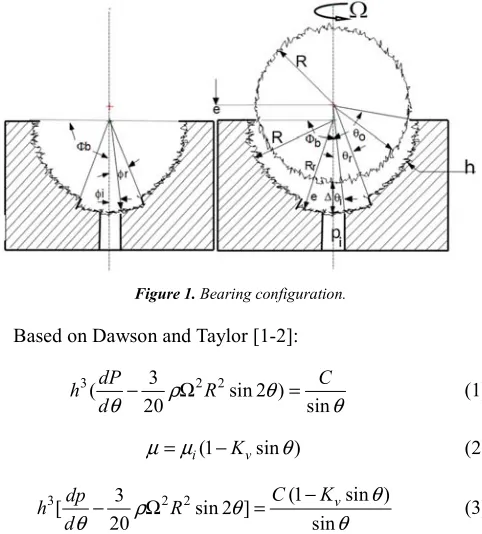
The modified form of Reynolds equation derived by Dowson and Taylor [1-2] and their suggested equation for the lubricant viscosity variation applicable to the hydrosphere Figure (1) have been adopted in this study.

Figure 1. Bearing configuration.

Based on Dawson and Taylor [1-2]:

3 3 2 2

( sin 2 )

20 sin

dP C

h R

dθ − ρΩ θ = θ (1)

(1 sin )

i Kv

µ µ= − θ (2)

3 3 2 2 (1 sin )

[ sin 2 ]

20 sin

v

C K

dp

h R

d

θ

ρ θ

θ θ

−

− Ω = (3)

(3)

2 2

3 2

(1 sin ) 3

sin 2 20

( 3 ) sin

v o o o

C k

dp

R

d h h

θ

_ρ

_θ

θ

σ

θ

−

= + Ω

+ (4)

3 2 2

1

3 2 2 2

4

( )(1 )

v

A

P dH S HdH

H b H H

Ak

dH

H b H H

− = − + − + + −

∫

(5)

2 2

2

2 ₂ ₂

2

1

{ ln(1 sec ) ln(tan( )}...

1 2

1 sin 1 1 sin

{ln( ) ln( )}

1 sin

2 ₁ _{1 sin}

2 cos

v

A

P b

b b

k A b

b _b _b

S B θ θ θ θ θ _θ θ = + + + + + − − + − ₊ _{+ +} − + (6) Where: i

P= p p ; H=h e_o =cosθ; A=C e P3 _i,σ_o e=σ

2 2

(3 40)

S=

ρ

Ω R , 3σ2 =b2, C= −6µ_iQ π

(1 sin )

dθ= − θ dH

3. Theoretical Solutions

3.1. Pressure Distribution

3.1.1. Recessed Zone

Following Yacout [4] in treating the recessed zone as a fitted type bearing of radius (R) and eccentricity (e_r):

( )r ( r )

h = e e h&A_r =αA

Equation (5) and its integration become:

( ) 3 2 2

1

3 2 2 2

4

( )(1 )

r

v

A

P dH S HdH

H b H H

Ak

dH

H b H H

α α − = − + − + + −

∫

(7)

2 2

( ) ₂ ₂

2

2 ₂ ₂

2

1

{ ln(1 sec ) ln(tan( )}...

1 2

1 sin 1 1 sin

{ln( ) ln( )}

1 sin

2 ₁ _{1 sin}

2 cos r v r A P b b b

A k b

b _b _b

S B α _θ _θ α θ θ θ _θ θ = + + + + + − − + − ₊ _{+ +} − + (8)

Applying the boundary conditions:

Atθ θ= _i→P_{( )}_r =1

Atθ θ= _r→P( )r =Pr

Then:

2 2 2

2 ₂ ₂

1 1

1 2 cos [ { ln(1 sec ) ln(tan( )}

1 2

1 sin 1 1 sin

{ln( ) ln( )}]

1 sin

2 ₁ _{1 sin}

r i i

v i i

i _i

B S A b

b b

k b

b _b _b

θ α θ θ θ θ θ _θ = + − + + + + + − − + − ₊ _{+ +} 2 2

2 2 2 2

2

2 2

2 2 2

2 2

(1 sec ) (tan( )

1 1

1 [ { ln ln }

(tan( )

1 2 (1 sec )

1 sin 1 sin

{ln( * )

1 sin 1 sin

2

1 sin 1 sin

1

ln( * )}]

1 1 sin 1 sin

2 (cos cos )

r r

r

i i

v r i

r i i r r i i r b P A

b b b

k b

b b

b b b

S θ θ α θ θ θ θ θ θ θ θ θ θ θ θ + = + + + + − + − + − + + + + − + + + + − + − (9)

3.1.2. Seat Zone

Applying the boundary conditions:

Atθ θ= _r→P=P_r

Atθ θ= e→P=0

Then:

2 2 2

2 ₂ ₂

1 1

2 cos [ { ln(1 sec ) ln(tan( )}

1 2

1 sin 1 1 sin

{ln( ) ln( )}]

1 sin

2 ₁ _{1 sin}

e e e

v e e

e _e

B S A b

b b

k b

b _b _b

θ θ θ θ θ θ _θ = − + + + + + − − + − ₊ _{+ +} 2 2 2 2 2 2

2

2 2

2 2 2

2 2

(1 sec ) (tan( )

1 1

[ { ln ln }

(tan( )

1 2 (1 sec )

1 sin 1 sin

{ln( * )

1 sin 1 sin 2

1 sin 1 sin

1

ln( * )}]

1 1 sin 1 sin

2 (cos cos )

r r

r

e e

v r e

r e e r r e e r b P A

b b b

k b

b b

b b b

S θ θ θ θ θ θ θ θ θ θ θ θ θ θ + = + + + − + − + − + + + + − + + + + − + − (10)

Equating the two equations (9) and (10) gives:

2 2

1 2

1 2 (cosS i cos e)

A L L θ θ + − = − Where: 2 2 1 2 2 2 2

2

2 2

2 2 2

(1 sec ) (tan( )

1 1

[ { ln ln }

(tan( )

1 2 (1 sec )

1 sin 1 sin

{ln( * )

1 sin 1 sin

2

1 sin 1 sin

1

ln( * )}]

1 1 sin 1 sin

r r

e e

v r e

r e e r r e b L

b b b

k b

b b

b b b

(4)

2 2

2 ₂ ₂ ₂ ₂

2

2 2

2 2 2

(1 sec ) (tan( )

1

[ { ln ln }

(tan( )

1 2 (1 sec )

1 sin 1 sin

{ln( * )

1 sin 1 sin

2

1 sin 1 sin

1

ln( * )}]

1 1 sin 1 sin

r r

i i

v r i

r i i r r i b L

b b b

k b

b b

b b b

θ θ α θ θ α θ θ θ θ θ θ θ θ + = + + + − + − + − + + + + − + + + + − Generally: 2 2 2 2 2

2 ₂ ₂

2

1

{ ln(1 sec ) ln(tan( )}... 1 2

1 sin 1 1 sin

{ln( ) ln( )}

1 sin

2 ₁ _{1 sin}

2 cos

v

A

P b

b b

A k b

b _b _b

S D α _θ _θ α θ θ θ _θ θ = + + + + + − − + − ₊ _{+ +} − + (11)

Where: ( 1)

( 1)

r

D B at

D B at

α

= <

= =

Hint:

This pressure formula covers the un-recessed bearing also when (α=1)

3.2. Load Carrying Capacity

From the Appendix (A1): 2

1 1 2 2

sin 2[( ) ( )]

W=

θ

+ a +b − b −a (12)

3.3. Temperature Distribution

From Elescandarany [4]:

2 2

2 4 2

( sin 2 ) ( ) 4 ( ) sin(2 )

0.21

( )

(2 sin 2 )

( ) sin sec (1 sin )

(2 sin 2 ) i

v

dP dP S

S p

dT _d _d

dP d c d Const k X dP d θ θ θ θ θ ρ _θ θ θ θ θ θ θ − + = − − + = − 1 1 2 2 4 160 ( ) n n i i i e T X

T T X

T T

S Const

p R K

θ θ µ ρ − ∆ = ∆ = + ∆ = = (13)

3.4. Frictional Torque

Following Yacout and Dowson [1-4]:

3 3

4 sin 4 sin

2 2 cos cos e r i r r r

m R d R d

e e θ θ θ θ θ θ πµ θ πµ θ θ θ = Ω

_∫

+ Ω

_∫

(1 sin )

i kv

µ µ= − θ

3 4

3

(1 sin ) sin cos 2

(1 sin ) sin cos r i e r v b i v k me z d e R k d e θ θ θ θ θ _{θ θ} θ π µ θ _{θ θ} θ − = Ω − +

∫

3 3

(1 sin ) sin

r i e r v b v k

M z d

h k d h θ θ θ θ θ _{θ θ} θ _{θ θ} − = − +

∫

The Integration could be found in the Appendix (A3) as:

b r s

M =z M +M (14) Where: 2 2 2 2 2 2 3 cos

[ ( 1) ln (cos ) ]

2 2 cos

[( 1){sin ln (tan sec )}

sin

{ln (sec tan ) sec tan } ]

2 3 r i r i r v M k θ θ θ θ θ _σ _θ σ θ σ θ θ θ σ _θ _θ _θ _θ θ = + − + − − − − + − + − − 2 2 2 2 2 2 3 cos

[ ( 1) ln (cos ) ]

2 2 cos

[( 1){sin ln (tan sec )} sin {ln (sec tan ) sec tan } ]

2 3 e r e r s v M k θ θ θ θ θ _σ _θ σ θ σ θ θ θ σ _θ _θ _θ _θ θ = + − + − − − − + − + − −

3.5. Volume Flow Rate

From [1-4]

Q=−A (15)

3.6. Friction Factor

From [1-4]:

F=M W (16) 3.7. Power Factor

From [1- 4]:

2 3 cos f e Q h W

π

θ

= (17)

3.8. Pump Power

From [3- 5]:

2 3 6

s t

p e

P π β Q

µ

(5)

3.9. Frictional Power

From [3- 5]:

4 2

2

f

R

P M

e

π Ω

= (19)

3.10. Total Losses

t p t

P =P +P (20)

3.11. Stiffness Factor

From [1- 4]:

_ _

( )

SF= − βW+βW (21)

4. Results

As previously mentioned, the main target of the research is to thermally examine the design of this type of bearings.

Mathematical expressions have been derived to examine the recessed bearing characteristics such as pressure

distribution, temperature distribution, load carrying capacity, flow rate, frictional torque, friction factor and stiffness factor. The bearing characteristics have been examined for the bearing with hemispherical and partially hemispherical seats. The recess effect on the bearing behavior has been also examined and an optimal design based on the minimum losses is performed.

These mathematical expressions could be considered as general expressions for the fitted type of bearings where they could also be applied to examine and design the un-recessed bearing.

5. Discussion

Studying the thermal behavior of the recessed fitted bearing in the presence of inertia and surface roughness, the visions of references [1-5] have been followed.

5.1. The Pressure Distribution

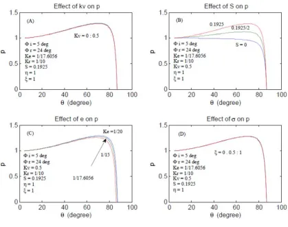
The pressure distribution under the effect of different parameters is represent by figures (2, 3)for a bearing with hemispherical and partial hemispherical seats.

Hemispherical Seat

(6)

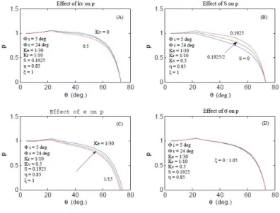
Partial Hemispherical Seat

Figure 3. Effect of different parameters.

5.1.1. The Effect of the Viscosity

From subfigures (2a, 3a) it could be observed that the viscosity has insignificant effect on the pressure in case of the hemispherical seat due to the high inertia while its effect could be appreciable in the case of the partial hemispherical seat due to lesser inertia.

5.1.2. The Effect of the Inertia

Subfigures (2b, 3b) show the pressure under the effect of the inertia which has a dominant role in increasing the pressure specially with the hemispherical seat despite its lesser effect with the partial hemispherical one. The inertia is represented by the speedparameter [1-4],

5.1.3. The Effect of the Eccentricity

The eccenrticity effect on the pressure is represented by Subfigures (2c, 3c) where it is clear that the pressure decreases with the increase in the eccentricity. This insignificant decrease inthe pressure despite the presence of the vicosity variation proovesthe highly stiffened bearing configuration designed in Yacout [3].

5.1.4. The Effect of the Surface Roughness

From subfigures (2d, 3d) it is clear that the two bearing configurations ’hemi and partial hemispherical seats’ haven’t been significantly affected by the surface roughness.

Comparing these results with those in Yacout [3-4] no remarkable difference could be observed despite the viscosity variability which leads to the prediction that the bearing stiffness will not be seriously affected by the viscosity

variation [4].

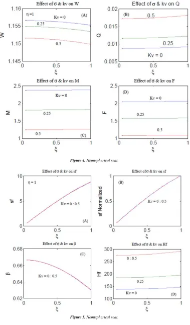
5.2. The Viscosity Effect on the Performance

The effect of the viscosity on the performance of a bearing with hemi and partial hemispherical seats is represented by figures (4-7).

Subfigures (4a, 6a) show the load decrease with the increase in both of the viscosity variation costant and the surface roughness where it could be easily predicted from the pressure figures.

It could be seen from the subfigures (4b, 6b) that the volume flow rate increases with the increase in the viscosity variation constant and the surface roughness parameter in turn the power factorsubfigures (5d, 7d)dependently increases where it could be sirectly predicted from the mathematical equation numbered (17).

Subfigures (4c, 6c) and subfigures (4d, dc) show decreasing inthe frictional tourque and the fricrion factor respectively.

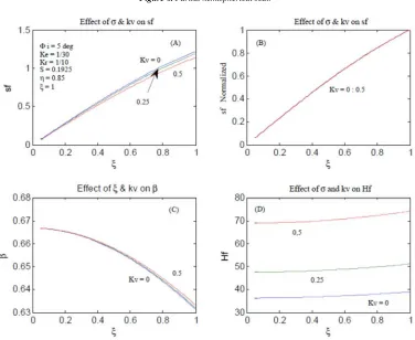
The stiffness factor, subfigures (5a, 7a), shows insignificant effect specially in case of the partial hemispherical seat at the high values of thesurface roughness parameter and when normalized, subfigures (5b, 7b), it showsconsistancy.

(7)

Figure 4. Hemispherical seat.

(8)

Figure 6. Partial hemispherical seat.

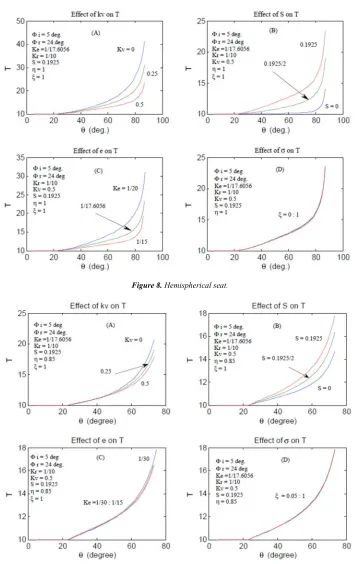
5.3. The Temperature Distribution

Figures (8, 9) represent the effects of the viscosity variation, the inertia, the eccentricity and surface roughness on the temperature distribution.

5.3.1. The Effect of the Viscosity

(9)

5.3.2. The Effect of the Inertia

Subfigures (8b, 9b) shows that the inertia plays an important role in raising the temperature where it is more efficient in case of the partial hemi spherical seat [4].

5.3.3. The Effect of the Eccentricity

Subfigures (8c, 9c) shows that the temperature is positively affected by the decrease in the eccentricity in case of the hemispherical seat while its effect could be considered

insignificat in case of the partial hemispherical sea.

5.3.4. The Effect of the Surface Roughness

Subfigures (8d, 9d) shows that the surface roughness has the least effect on the temperature where it could be practiclly ignored [4].

(10)

5.4. The Effect of the Recess

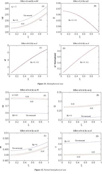
Figures (10-13) represent the effect of the recess on the bearing performance.

5.4.1. The Load Carrying Capacity

Subfigures (10 a, 12 a) show notable increase in the load reaches to about % 2 in case of the hemispherical seat while it reaches to about % 30 in case of the partial hemispherical one. Deepening the recess gets insignificant increase in the load.

5.4.2. The Volume Flow Rate

Subfigures (10 b, 12 b) show increase in the volume flow rate where it is comperatively more in case of the partial hemispherical seat. Increasing the recess depth has insignificant effect.

5.4.3. The Frictional Torque and the Friction Factor

Subfigures (10 c, d & 12 c, d) show decrease in the frictional torque and the friction factor and the decrease is relatively more in case of the partial hemispherical seat. Deepening the recess has insignificant effect.

5.4.4. The Power Factor

Subfigures (11 a, 13 a) show decrease in the power factor but it could be very small in case of the hemispherical seat comparatively to that in case of the partial hemispherical one. High values of the recess depth have insignificant effect.

5.4.5. The Central Pressure Ratio

Subfigures (11 b, 13 b) show approximately no effect in case of the hemispherical seat and notable decrease in case of the partial hemi-spherical one specially at higher values of the surface roughness parameter. Deepening the recrss has insignificant effect.

5.4.6. The Stiffness Factor

Subfigures (11 c, 13 c) shownotable decrease in case of the partial hemi-spherical seat specially at higher values of the surface roughness parameter and insignificant effect in case of the hemispherical seat. Normalizing the Stiffness, factor, subfigures (11 d, 13 d) show no effect which reveals the bearing consistancy. Deepening the recrss has insignificant effect.

(11)

(12)

5.5. The Bearing Design

As in Yacout [3], abearing with the same dimensions is re-desigend under the same conditions in the presence of the fluid variable viscosity.

50

R= mm, 5

o i

φ = , 24

o r

φ = ,η =(1& 0.85),

ξ

=0.05,

(1 10 )

r

K = ,N=100rps,S=0.1925 p_s =5 1x o N m5 2,

2 3

β = ,

ρ

=867 N s. 2 m4 ,

µ

=0.068 N s m. 2,

2 2

1880 . o

v

C = m s c ,K_v =(0 & 0.5)

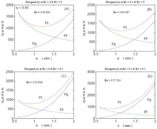
5.5.1. Determening the Eccentrecity

Figures (14, 15) show losses at different eccentricities for the fitted type covering its eight possible cases. Subfigures (14 a, b & 15 a, b) for the bearing (with and without) recess, (hemi and partial hemi) seats at constant viscosity. Subfigures (14 c, d & 15 c, d) for the bearing (with and without) recess, (hemi and partial hemi) seats at variable viscosity.

The optimum eccentricity for each is determined at the minimu total Power losses from the graphs [14, 15].

(13)

5.5.2. The Bearing Characteristics and Behavior

The concerned bearing in this part of the research is the recessed one at variable viscosity with heni snd partial hemispherical seats.

Figures (16-21) represent the designed bearing performance and its behavior if operated under conditons differ from the those of the design.

5.5.3. Checking the Bearing Design

To check the bearing designed in Yacout [3], Subfigures (14 a, b & 15 a, b) show the eccentricity ratios (Ke = 1/17.606) forboth

the un-recessed and recessed hemispherical seats which coincide with those in Yacout [3] and (Ke = 1/41.831)

forun-recessedpartial hemispherical seat and (Ke = 1/43.367) for

recessedpartial hemispherical seat respectively. In Elescandarany [4] the study doesn’t handle the design.

(14)

(15)

(16)

6. Conclusion

This part of the research concerns with the recessed fitted type of bearings when the fluid film viscosity is variable in the presence of inertia and surface roughness.

The main items could be abstracted from the aforementioned discussion are:

a)Deriving mathematical expressions cover this type of bearings with its different configurations and whether the fluid film viscosity is constant or variable.

b)Optimal design based on the minimum losses. c)Checking bearing design with constant viscosity.

Future Work

The 3rd part of the research handles the design of the fitted type with its different configurations comparing between their performances revealing the advantages and drawbacks of each.

Appendix

A1– The Load Carrying Capacity Derivation

Following Dowson and Yacout [1-4]:

2 2 2

( )

2

sin 2 sin( ) cos( )

2 sin( ) cos( )

r i o

r

i i r

w R p R p d

R p d

θ

θ θ

θ

π θ π θ θ θ

π θ θ θ

= +

_∫

+

∫

2

( )

sin 2 sin( ) cos( ) 2 sin( ) cos( )

e r

i r

W P d P d

θ θ

θ θ θ θ θ θ θ

= +

_∫

+

_∫

2

1 2

sin _i 2( )

W=

θ

+ F +F

Where:

1 ( )sin( ) cos( )

r i

r

F P d

θ

θ θ θ

=

_∫

2 sin( ) cos( )

e r

F P d

θ

θ θ θ

=

_∫

The integration of (F2) could be directly found in Yacout [3, 4] as:

(17)

2 2 2

2 2

1 ₂ ₂ ₂

2

4 2

2

cos sin

[ ln ( cos ) ln (sin )

4 ( 1) 2( 1)

cos

ln (cos )] [cos ] [ cos ]

2 2

2

e e

r

e r r

b

a A b

b b b

S B b θ θ θ θ θ θ θ _θ θ _θ θ _θ _θ _θ + = + − − + + + −

2 2 2 2

2 ₂

2 2

(cos ) (1 sin ) cos ( 1 sin )

[ ln ( ) ln ]

2 (1 sin )

4 2 1 ( 1 sin )

e r

v

K A b b

a

b b b

θ θ θ θ θ θ θ _θ − + + − = − + ₊ _{+ +}

And the integration of (F1) has exactly the same form as: F1 = b1 +b2

2 2 2

2 2

1 ₂ ₂ ₂

2

4 2

2

cos sin

[ ln ( cos ) ln (sin )

4 ( 1) 2( 1)

cos

ln (cos )] [cos ] [ cos ]

2 2

2

i r r

r i i

r

b

b A b

b b b

B S b θ θ θ θ θ θ θ _θ θ _θ θ _θ _θ _θ + = + − − + + + − 2 2 ₂

2 2 2

2 2

(cos ) (1 sin )

[ ln

2 (1 sin ) 4

cos ( 1 sin )

( ) ln ]

2 1 ( 1 sin )

r i v r K A b b b b b b θ θ θ θ θ θ θ θ − = − + + + − + + + r

A =αA

Hence:

2

1 1 2 2

sin 2[( ) ( )]

W=

θ

+ a +b − b −a

A2 – The Integration of the Frictional Torque

3 3

(1 sin ) sin e(1 sin ) sin

r

i r

v v

b

k k

M z d d

h h θ θ θ θ θ θ _θ θ θ _θ − − =

_∫

+

_∫

Following Yacout [3, 4]:

2 2 2 2

3 3 1 cos ( ) cos h E h h σ θ σ θ + +

= = (Fitted)

Taking the expectation of both sides:

2 2 3

3

2 2 3

3

(cos )(1 sin ) sin

cos

(cos )(1 sin ) sin

cos r i e r v b v k

M z d

k d θ θ θ θ θ σ θ _{θ θ} θ θ σ θ _{θ θ} θ + − = + − +

∫

b r s

M =z M +M

2 2 3

3

(cos )(1 sin ) sin

cos r i v r k M d θ θ θ σ θ _{θ θ} θ + − =

_∫

2 2 3

3

(cos )(1 sin ) sin

cos e r v s k M d θ θ θ σ θ _{θ θ} θ + − =

_∫

The integration could be found in Yacout [3, 4] as:

2 2 2 2 2 2 3 cos

[ ( 1) ln (cos ) ]

2 2 cos

2 3 r i r i r v M K θ θ θ θ θ _σ _θ σ θ σ θ θ θ σ _θ _θ _θ _θ θ = + − + − − − − + − + − − 2 2 2 2 2 2 3 cos

[ ( 1) ln (cos ) ]

2 2 cos

2 3 e r e r s v M K θ θ θ θ θ _σ _θ σ θ σ θ θ θ σ _θ _θ _θ _θ θ = + − + − − − − + − + − − 2 2 ₂

2 2 2

2 2

(cos ) (1 sin )

[ ln

2 (1 sin )

4

cos ( 1 sin )

( ) ln ]

2 1 ( 1 sin )

r i v r K A b b b b b b θ θ θ θ θ θ θ θ − = − + + + − + + +

References

[1] Dowson D. and Taylor M. 1967, “Fluid inertia effect in spherical hydrostatic thrust bearings”, ASLE Trans. 10, 316- 324.

[2] Dowson D. and Taylor M. 1967, “A Re- Examination of hydrosphere performance”, ASLE Trans. 10, 325- 333. [3] Ahmad W. Yacout, Ashraf S. Ismaeel, Sadek Z. Kassab, 2007,

“The combined effects of the centripetal inertia and the surface roughness on the hydrostatic thrust spherical bearing performance”, Tribolgy International Journal Vol. 40, No. 3, 522-532.

[4] Ahmad W. Y. Elescandarany, 2018, “The Effect of the Fluid Film Variable Viscosity on the Hydrostatic Thrust Spherical Bearing Performance in the Presence of Centripetal Inertia and Surface Roughness (Part 1 Un-recessed fitted bearing)”, The International Journal of Mechanical Engineering and Applications Vol. 6, No. 1, pp. 1-12.

[5] Essam Salem and Farid Khalil, Variable viscosity effects in Externally Pressurized spherical Oil Bearings, Journal of Wear 1978, 50, 221-235.

[6] Keith Brockwell, Scan Decamillo and Waldemar Dmochowski, 2001, “Measured temperature characteristics of 152 mm diameter pivoted shoe journal bearings with flooded lubrication”, Tribology Transaction vol. 44, No. 4, 543-550. [7] B Glavatskih and S De Camillo, 2004, “Influence of oil

viscosity grade on thrust pad bearing operation”, Proc. Inst. Mech. Eng. Vol. 218, part j: J. Engineering tribology.

(18)

[9] Ivan Filipović and DževadBibić, 2010, “Impact of oil viscosity on functional parameters of journal bearings in internal combustion engines”, Gorivaimaziva, 49, 4, 334 - 351 [10] Srinivasan V. 2012, “Analysis of Static and Dynamic Load on the Hydrostatic Bearing with Variable Viscosity Affected by the Environmental Temperature”, Journal of Environmental Research and Development Vol. 7, No. 1A, 346-353.

[11] Srinivasan V. 2013, “Analysis of Static and Dynamic Load on Hydrostatic Bearing with Variable Viscosity and Pressure”, Journal of Environmental Research and Development Vol. 6 (6s), 4777-4782.

[12] N. B. Naduvinamani and Archana K. Kadadi, 2013, “The effect of viscosity variation on the micro-polar fluid squeeze film lubrication of a short journal bearing”, Advances of

Tribology Journal, Vol. 2013, Article ID 743987.

[13] Shigang Wang, Xianfeng Du, Mingzhu Li, Zhongliang Cao, Jianjia Wang, 2013,“Analysis of temperature effect on the lubricating state of hydrostatic bearing”, Journal of Theoretical and Applied Information Technology Vol. 48, No. 2, 817-821.

[14] B. Bouchehit, B. Bou-Saïd and M Garcia, 2016, “Static and dynamic performances of refrigerant- lubricated foil bearings”, 7th international conference on advanced concepts in mechanical engineering.