Developments in stylus profilometry

(1)

Developments in Stylus Profîlometry

A Thesis Submitted for the Degree

of

Doctor of Philosophy of the University of London

by

Ho Soon Yang

Optical Science Laboratory

Department of Physics and Astronomy

University College London

University of London

(2)

ProQ uest Number: U 642019

INFORMATION TO ALL U SE R S

The quality of this reproduction is d ep en d en t upon the quality of the copy subm itted.

In the unlikely even t that the author did not sen d a com plete manuscript

and there are m issing p a g e s, th e se will be noted. Also, if material had to be rem oved, a note will indicate the deletion.

uest.

ProQ uest U 642019

Published by ProQ uest LLC(2015). Copyright of the Dissertation is held by the Author.

This work is protected against unauthorized copying under Title 17, United S ta tes C ode. Microform Edition © ProQ uest LLC.

ProQ uest LLC

789 East E isenhow er Parkway P.O. Box 1346

(3)

(4)

Abstract

(5)

List of Figures

Figure 1.1: Layout o f a conventional Fizeau interferometer with the phase shifter, reproduced from Burge (Burge 1995)... 23 Figure 1.2: Theoretical calculation o f fringe number per pixel o f detector along the centre

line with respect to the best-fit sphere, when the Gemini secondary mirror (convex) is tested with Fizeau interferometry. The pixel number o f detector is 512x512. The dotted line is at h alf fringe, under which the phase o f the fringe can be unwrapped correctly by PSI techniques... 24 Figure 1.3: The optical layouts o f various null configurations, (a) Offher null test, (b)

Offtier two-mirror test, (c) Hindle test, and (d) modified Hindle test. C\ and C2

are conjugate points o f convex hyperboloid. C2 is also coincident to the centre o f

curvature o f Hindle sphere in (c) and the reference surface o f the meniscus lens in (d)...25 Figure 1.4: OPD construction o f TWPSI technique, reproduced from Optical Shop

Testing (Malacara 1992). The circles are spaced X\ and the crosses X2...27

Figure 1.5: Schematic diagram o f a quantitative knife-edge testing, reproduced by the kind permission of Kim (Kim 1998)...30 Figure 1.6: The schematic diagram o f the old SPLOT (1996)... 32 Figure 2.1: The comparison of the surface profiling techniques in terms o f spatial

wavelength range, reproduced from Bennett (Bennett 1985). Numbers in parentheses are the range o f heights. The wavelength used in TIS (total integrated scattering) technique is 632.8 nm... 35 Figure 2.2: The conceptual diagram o f a modem stylus profîlometry... 36 Figure 2.3: Schematic diagram o f Form Talysurf traverse unit with the laser

(11)

Figure 2.5: The typical plunger type stylus system, reproduced from Leadbeater

(Leadbeater 1990)... 38

Figure 2.6: Diagrams o f two different reference types: (a) a skid reference (b) a separate reference...44

Figure 2.7: The principle o f reversal method, reproduced from Estler (Estler 1985). (a) normal orientation and (b) reversed orientation: reference is rotated 180° about its long axis... 45

Figure 2.8: The schematic diagram o f the optical system in LTP, reproduced from Irick (S. C. Irick 1992)...46

Figure 2.9: Geometry for the swing arm profilometer (Burge 1997)...47

Figure 3.1 : The block diagram o f the SPLOT...53

Figure 3.2: The probe system for SPLOT (Hubbard 1996)...54

Figure 3.3: The guidance system o f probe system in SPLOT (Hubbard 1996)...55

Figure 3.4: The optical layout o f interferometric distance measurement system adapted in SPLOT...57

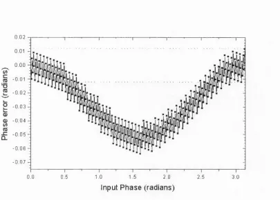
Figure 3.5: Simulated phase error between the calculated phase in the interpolation programme and input phase, when the phase difference o f two output signals from interferometry is about 87 degrees. 256 interpolation was selected. The dotted line is the resolution o f phase calculation... 59

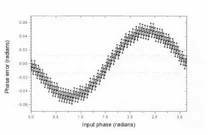
Figure 3.6: Simulated phase error between the calculated phase by the interpolation programme and input phase, when one output signal from the interferometer is 10% bigger than the other. 256-interpolation was selected. The dotted line is the resolution o f the phase calculation... 61

Figure 3.7: The diagram o f flexure system o f SPLOT...63

Figure 3.8: Error signal generation of quadrant diode...64

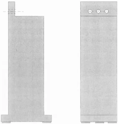
Figure 3.9: New Cervit pillar for laser reference system... 66

Figure 3.10: Side view o f the layout for generating reference beam and horizontal interferometer, installed on the new cervit pillar... 66

Figure 3.11 : Schematic diagram o f SPLOT after some preliminary modifications... 67

Figure 4.1 : The typical drifting trend o f the height measurement... 69

(12)

Figure 4.3: Fast recording o f the height variation (graph (1)) and its derivative (graph (2)) during the movement o f the probe system. The speeds o f case (a), (b) and(c) are the same as the Figure 4.2...73 Figure 4.4: The conceptual picture o f explaining why the height apparently rises after the

probe hits the surface. The solid configuration is just when the probe hits the surface and the dotted one is when the motion o f probe stops...74 Figure 4.5: Experimental result o f height error variation according to the different driving

speed...75 Figure 4.6: The speed variation o f the MM when it travels fi-om top to bottom o f its travel

length... 76 Figure 4.7: The conceptual picture to show how the stopping position o f probe system

varies according to the surface slope to be measured: (a) upward slope (b) downward slope... 77 Figure 4.8: The assembly o f the probe using a Ruby ball... 78 Figure 4.9: Drawing o f the new probe arm... 79 Figure 4.10: The assembly o f the probe, retro-reflector and counterweight on the probe

arm... 79 Figure 4.11 : The optical switch and movable pod on the body o f the probe system... 82 Figure 4.12: Experimental result o f monitoring the probe motion (boxed points) and the

signal from the optical switch (circled points)... 82 Figure 4.13: Proposed clamping method for the thin wire in the new probe system... 83 Figure 4.14: Pictures o f the new probe system assembled on the SPLOT: (a) front view,

(b) side view...85 Figure 4.15: The speed variation o f the MM with a new controller... 87 Figure 4.16: The flowchart for the CPF measurement... 88 Figure 4.17: Monitoring the height variation when the probe contacts the optical flat with

zero slope. Graph (a) is the continuous recording o f the probe motion and graph (b) is the difference between two successive data in graph (a)... 90 Figure 4.18: The height variations at four different speeds: 30 pm/sec (■), 120 pm/sec

(•), 170 pm/sec ( ^ ) , a n d 260 pm/sec ( ^ ) ... 91 Figure 4.19: Monitoring the vertical displacements when the probe contacts the optical

fiat with 8.1 degree o f slopes. Graph (a) is the continuous recording o f the probe motion and graph (b) is the differences between two successive data in graph (a)..93

(13)

Figure 4.20: The repeatability test on the zero slope surface. The boxed points come from CPF measurement and the circle points from final state measurement 95 Figure 4.21 : The repeatability test on the 8.1 degrees sloping surface. The boxed points

come from CPF measurement and the circle points from final state measurement. 95 Figure 4.22: The repeatability test on zero slope surface (square points) and the drifting

measurement (solid line)...96 Figure 5.1 : Schematic diagram o f horizontal motion system for SPLOT... 101 Figure 5.2: Schematic diagram o f winding o f the cord around the motor shaft...101 Figure 5.3: The oscillatory motion o f the horizontal system at various positions on the

granite beam: (a) 110 cm, (b) 70 cm and (c) 30 cm away from the motor...103 Figure 5.4: The Fourier transform o f Figure 5.3... 104 Figure 5.5: Theoretical variation o f the resonant frequency o f the horizontal system 106 Figure 5.6: The picture o f the air bag used in SPLOT... 108 Figure 5.7: Translation, pitch and roll mode o f the system... 108 Figure 5.8: Environmental vibrations o f various frequencies, reproduced from Melles

Griot (Melles Griot )... 110 Figure 5.9: The experimental set-up (backside view) o f viscous damping for the air

bearing motion...I l l Figure 5.10: The structure o f the belt used in the horizontal system... 112 Figure 5.11 : The oscillatory motion o f the horizontal system when the stainless steel belt

is used instead o f the polyethylene cord. Graph (a) is the sampling data from DSP (1.23nm resolution), (b) power spectrum o f (a)...113 Figure 5.12: The repeatability test on 15.6 degrees sloped surface at stationary state o f

horizontal drive system. The square points are the height measurement and the circled ones are the horizontal measurement... 114 Figure 5.13: Differences o f two successive vertical measurements (square points) and

expected vertical differences derived from the difference o f two successive horizontal measurements (circled points)...116 Figure 5.14: The error o f two differences at each sampling point in Figure 5.13...116 Figure 5.15: Speed fluctuation o f the horizontal motion driven with two different speeds:

(a) 400 pm/sec and (b) 570 pm/sec...118 Figure 5.16: The vibration o f the probe during the horizontal motion at the speed o f 570

(14)

Figure 6.1: Conceptual diagram o f the new laser reference system for one channel. The

other channel is the replica o f this one... 124

Figure 6.2: The circuit diagram o f QD electronics... 125

Figure 6.3: The circuit diagram o f pre-amplifier...127

Figure 6.4: Schematic diagram o f the relay and relay electronics...128

Figure 6.5: The circuit diagram o f PZT amplifier... 128

Figure 6.6: Experimental result o f gain curve o f high voltage amplifier against the frequency o f input voltage. The dotted line is the 3dB line...130

Figure 6.7: Two-axis flexure system developed by Hubbard (Hubbard 1996)... 131

Figure 6.8: Experimental set-up o f eddy current sensors for measuring the displacement o f the QD...132

Figure 6.9: The variation o f voltage o f vertical channel o f the QD according to the change o f the QD position vertically...133

Figure 6.10: The variation o f voltage o f the horizontal channel o f the QD according to the change o f the QD position horizontally with respect to the table... 133

Figure 6.11: Block diagram o f the reference system when the PZT operates... 134

Figure 6.12: The simulation o f transient responses o f the PZT (circle points) to the step perturbation (sold line)...135

Figure 6.13: The horizontal (square points)/vertical (circle points) displacement o f the QD for the vertical (bottom x-axis)/horizontal (top x-axis) flexure movement 137 Figure 6.14: The conceptual diagram to show the arcuate motion according to the longitudinal displacement (Ax) in a single-axis flexure system...138

Figure 6.15: New bracket for removing the slip between the horizontal PZT and MM. The centre part o f the bracket is not a material... 140

Figure 6.16: The cross-talk o f the flexure system after modification... 140

Figure 6.17: The vertical (upper lines) and horizontal (lower lines) displacement o f the reference beam on the QD, when the air bearing is off. (a) there was no polythene curtain, (b) there was a single polythene curtain, and (c) there was a single polythene curtain and a second polythene cover on the instrument... 143

Figure 6.18: The typical vertical (upper lines) and horizontal (lower lines) o f the reference beam displacement from the centre o f the QD when the air bearing is on, with conditions (a) there was a single polythene curtain and (b) there was a single polythene curtain and cover on the instrument... 144

(15)

Figure 6.19: The picture o f experimental set-up to prevent the direct effect o f leaked air from the air bearing to reference beam path...145 Figure 6.20: The typical variation o f height in open loop operation, when the probe

system was stationary in the air and the polythene shielding was used... 146 Figure 6.21: The typical variation o f height in closed loop operation, when the probe

system was stationary in the air and the polythene shielding was used... 147 Figure 6.22: The generation o f step error function to the vertical flexure o f reference

system. The vertical PZT loses control at point ‘A ’ and regains it at point ‘B ’ manually...149 Figure 6.23: The magnified picture o f Figure 6.22 around event ‘B ’. The dotted line is the

original height value... 150 Figure 6.24: The difference between the original heights and flnal heights after the

compensation completed. The time interval between two events was about 2 seconds, so that the amount o f step error is about 0.5 pm ... 151 Figure 6.25: The repeatability test on the flat surface with zero slope when the laser

reference system is operated... 152 Figure 6.26: The repeatability test after the movement o f vertical flexure was

compensated... 153 Figure 7.1: The picture o f surface contour o f sample flat using WYKO 6000... 157 Figure 7.2: Two-dimensional profile o f the sample flat along the line which SPLOT

traces to measure... 157 Figure 7.3: Profile measurements o f the sample flat with the reference system enabled.

Square and circle points are results by SPLOT and the solid line is the profile produced by the WYKO 6000... 158 Figure 7.4: Profiles o f two scans o f the sample flat without the reference system enabled.

The solid line is the profile produced from the WYKO 6000... 159 Figure 7.5: An air bearing carriage loaded on the granite beam. The direction o f motion

is along the x-axis. The air bearing has error motions related to each o f the six degrees o f freedom. The centre o f the rotational motion is placed on the centre o f the air bearing... 161 Figure 7.6: The pitch angle o f the granite beam (upper) and its integration (lower) to

(16)

Figure 7.7: The effect o f the angular error. The dotted line is the original configuration and the solid line is the configuration after the rotation o f the carriage...163 Figure 7.8: The schematic diagrams o f the roll error o f the air bearing (end view), (a)

configuration (b) simplified diagram o f (a). The short dotted line and the solid line represent situations without and with the roll error ( 0 x ) . The long dotted line

in (b) represents the situation when the reference system operates. The circle, square and triangle points represent centres o f the roll motion, the beam splitter, and the QD respectively... 164 Figure 7.9: The roll error o f the carriage along the granite beam...165 Figure 7.10: Picture o f key components o f SPLOT (side view)... 167 Figure 7.11 : The schematic diagrams o f the pitch error o f the air bearing (side view), (a)

simplified configuration, (b) geometrical configuration, and (c) the motion o f the retro-reflector (★) in the horizontal interferometer. The long dashed line in (b) is the final configuration after the reference system compensated the QD position error... 167 Figure 7.12: The schematic diagrams o f the yaw error o f the carriage (top view), (a)

simplified configuration, (b) geometrical configuration (only beam splitter (★)and retro-reflector (■) were considered)... 169 Figure 7.13: Conceptual diagrams o f differential height measurement method, (a) the

original differential height measurement and (b) the simplified method for evaluating the differential height measurement with only one sphere... 172 Figure 7.14: The picture o f surface contour o f the sample sphere using WYKO 6000... 174 Figure 7.15: The 2-D profile o f the residual errors o f the sample sphere from the

reference sphere, along the line which SPLOT traces to measure...175 Figure 7.16: Profile measurement o f the sample sphere... 176 Figure 7.17: Residual errors o f the sample sphere, which were generated by subtraction

o f the best-fit sphere from the original data. Square and circle points are measurements on the no-tilt surface and tilted surface by SPLOT respectively. The solid line is the deviation from the reference sphere produced by WYKO 6000... 177 Figure 7.18: The cubic spline interpolation to the residual errors o f no-tilt measurement. 179

(17)

Figure 7.19: Differences o f best-fit curves o f two measurements (upper) and residuals generated by the subtraction o f the best-fit linear line from the differences (lower)...180 Figure A .l: The effect o f the tilt motion o f the probe system, (a) geometry o f the probe

system and (b) geometry o f the tilt motion... 188 Figure B .l: (a) Schematic diagram o f the horizontal drive system, (b) The simplified

modelling o f the horizontal driving system...191 Figure B.2: The dynamic magnification o f the system... 193 Figure C .l: Calculated variation o f the refractive index o f the air for typical laboratory

temperature changes (20-25 °C) at 1013 mbar o f the air pressure...196 Figure C.2: Calculated variation o f the refractive index o f the air as air pressure changes

at 20 °C...196 Figure C.3: Calculated variation o f the refractive index o f air as relative humidity

(18)

List of Tables

Table 1.1 : The primary and secondary mirror types o f reflecting telescopes... 21 Table 1.2: Characteristics o f very large telescopes (Kim 1998)...21 Table 3.1: Theoretical maximum frequency o f signal and maximum velocity o f moving

arm for the different level o f interpolation...62 Table 4.1 : The SD o f repeatability test at three different driving speed... 70 Table 4.2: Comparison o f dimensions o f each parameters o f the probe system and

theoretical estimation o f the effect of the overshooting o f the MM. In parenthesis is the result when the position o f retro-reflector is on the top o f the probe tip and other dimensions are not changed in the old system...80 Table 4.3: The comparison o f heights measured by CPF.exe and the final state

measurement at four different driving speeds... 91 Table 4.4: Comparison o f the l a o f the repeatability test with CPF.exe and the final

value measurement for the new probe system and the old probe system. The result o f the old probe system came from Figure 4.2... 96 Table 7.1 : The dimensions o f variables o f Figure 7.11... 168 Table 7.2: Comparison o f the estimated height errors due to rotational errors o f the air

bearing carriage. Target surfaces are the nominal fiat and curved surface (Gemini secondary mirror). The numbers in parenthesis are the original Abbe errors (lateral displacement o f the probe tip on the surface)... 171 Table 7.3: Notations and their definitions used in the demonstration o f the differential

height measurement method with one sphere... 173 Table C.l : Measurement errors for the variations o f the environmental conditions... 198

(19)

Glossary and symbols

ADC Analogue to Digital Converter

CCPM Computer Controlled Polishing Machine

CGH Computer Generated Hologram

CPF Contact Point Finding

DAC Digital to Analogue Converter DSP Digital Signal Processor

FEA Finite Element Analysis

KAIST Korea Advanced Institute o f Science and Technology MAI Multiple Annular Interferometry

MM Motor Mike

NPL National Physical Laboratory in UK

OPD Optical Path Difference

OSL Optical Science Laboratory at the UCL

PC Personal Computer

PSI Phase Shifting Interferometry

P-V Peak to Valley

QD Quadrant Diode

RMS Root-Mean-Square

ROC Radius O f Curvature

SNI Sub-Nyquist Interferometry

(20)

SUT Surface Under Test

TWPSI Two-Wavelength Phase Shifting Interferometry UCL University College London

a Standard Deviation

(21)

chapter 1 Introduction

1.1 Astronomical background

Up to the end o f the Middle Ages, the most important means o f observation in astronomy was the human eye. The telescope was invented in Holland at the beginning o f the 17^*’ century, and in 1609, Galileo Galilei made his first astronomical observations with his new telescope o f a converging objective lens and a diverging eyelens.

With advances in astronomy, astronomers needed larger telescopes since the light collecting power is a function o f the telescope diameter D as 7iD^/4, and according to Lord Rayleigh’s criterion (Smith 1990), the diffraction limited angular resolution is also increased by increasing the diameter, or

0 = 1.22X/D (radians), (1.1)

where X is the wavelength o f light.

(22)

Reflecting telescopes Primary mirror Secondary mirror

Newtonian Concave paraboloid Flat

Gregorian Concave paraboloid Concave ellipsoid

Cassegrain Concave paraboloid Convex hyperboloid Ritchey-Chretien Concave hyperboloid Convex hyperboloid

Table 1.1: The primary and secondary mirror types o f reflecting telescopes.

Telescopes Gemini VLT Subaru LET Keck

Number 2 4 1 1 2

Diameter 8 m 8 m 8.3 m 2x8.4 m 10 m

Type RC RC RC Cassegrain RC

F/# primary 1.8 1.8 1.8 1.14 1.75

Conic const. -1.003756 -1.004616 -1.0

Table 1.2: Characteristics o f very large telescopes (Kim 1998).

Therefore, all the m odem large telescopes are reflectors with aspheric surfaces. Table 1.1 shows the mirror types o f several kinds o f reflecting telescope and Table 1.2 lists characteristics o f very large telescopes (8 m class).

However, aspherics are not easy to make as well as test. While a spherical mirror can be polished with tools o f the same radius o f curvature, an aspheric surface should be polished with tools o f various diameters and radii o f curvature according to the polished zonal area o f surface. It takes much time to make, compared to the same diameter o f spherical mirror.

Testing an aspheric is even more problematic. The most commonly used testing method for spherical mirror, interferometry, would fail in testing even a mild aspheric mirror since it would generate too many fringes to analyse in the resulting

(23)

interferogram. Using null correctors is one o f the most frequent methods to reduce the fringe number without losing the measurement accuracy. However, this method sometimes led to the wrong result. One significant example o f those errors occurred at the testing o f the primary of the Hubble Space Telescope (HST) (L. Allen 1990). It was tested with a reflective null corrector consisting o f a field lens and two spherical mirrors. Two spherical mirrors compensated the spherical aberration o f the primary mirror so that the interferometric set-up was possible. However, the null corrector used was not a correct one due to a measurement error in its manufacture. It resulted in the form error o f the primary mirror.

The secondary mirrors for large telescopes are often convex, highly aspheric, and large (up to 1.7 m in diameter). Since the convex surface reflects the incident beams to be divergent, to test the secondary mirror is sometimes more difficult than to test the primary one, even though the size o f the secondary mirror is smaller than that o f the primary one.

In conclusion, in spite o f many advantages o f using aspherics in the large telescopes, the difficulty in testing aspherics increases the cost and risk o f telescope projects.

1.2 Technical background

1.2.1 Conventional Fizeau Interferometry

Conventional testing methods o f large optics are mainly to use the interferometry. The interferometry generates the interferogram, the optical phase difference (OPD) between the test surface and the reference surface. The image device digitises the fringes, and the fringe analysis system finds the phase information from them. The recent fringe analysis system such as WYKO 6000 (WYKO ) uses the phase shifting interferometry (PSI) (J. H. Bruning 1974; J. E. Greivenkamp 1992), which measures the phase to 7t/25~tc/250. Several algorithms used in PSI techniques are well explained in Optical Shop Testing (Malacara 1992). The deviation o f the test surface from the reference surface is then given by.

I n I

(24)

Reference surface

Phase shifter

▼ r Laser

BS C ollim ator

Im aging lens ^

T est surface

CC D cam era

Figure 1.1: L ayout o f a conventional Fizeau interferom eter w ith the phase shifter, reproduced from B urge (Burge 1995).

Flow ever, w hen the surface is severely aspheric, the conventional direct interferom etric testings fail due to m any fringes in one pixel o f the detector. O ne exam ple is show n here for the secondary m irror o f the G em ini telescope, w hich is the m ain case study throughout this thesis. Its diam eter is 1.022 m, the conic constant is -1 .6 1 2 8 9 8 , and the paraxial radius o f curvature is -4 1 9 3 .0 6 8 5 m m (H ansen 1994). L et us suppose that it is tested using the H e-N e laser and a detector w ith 512x512 pixels in a Fizeau interferom etry set-up o f w hich layout is show n in Figure 1.1.

Figure 1.2 show s the theoretical fringe num ber per pixels o f the detector along the centre line w ith respect to the best-fit sphere. The fringe num ber per pixel is m axim um 5.3 at the periphery o f the m irror. T his is ten tim es beyond the N y quist frequency o f the detector (tw o detector elem ents per fringe), w hich degrades the m odulation o f the fringe. A lso, since conventional PSI assum es that the phase difference betw een pixels is less than ti (or h a lf fringe) due to 27t am biguity (J. E. G reivenkam p 1992), a surface generating fringes m ore than the N yquist frequency cannot be correctly reconstructed. Therefore, m ost o f the area o f the G em ini secondary m irror cannot be tested w ith the conventional Fizeau interferom etry w ith PSI teclinique.

To test the optics w ith large asphericity, various m ethods have been developed such as null testing (H indle 1931; F. A. Sim pson 1974; O ffner 1978), S ub-N yquist Interferom etry (SN I) (G reivenkam p 1987; J. E. G reivenkam p 1992; G reivenkam p 1996), tw o-w avelength phase shifting interferom etry (T W PSI) (Y. Y. C heng 1984; K. C reath 1985), sub-aperture testing, etc. B rie f descriptions o f these m ethods are follow ed.

(25)

</)

0)

&

5

(D

I

S:

O)

c

6

5

4

3

2

1

0

1 0 0 20 0 300

Pixel number

400 5 00

F igure 1.2: T heoretical calculation o f fringe num ber per pixel o f d etector along the centre line w ith respect to the best-fit sphere, w hen the G em ini secondary m irror (convex) is tested w ith Fizeau interferom etry. The pixel num ber o f d etector is 512x512. The dotted line is at h a lf fringe, under w hich the phase o f the fringe can be unw rapped correctly by PSI techniques.

1.2.2 Null testing

The m ost frequently used m ethod in highly accurate aspheric testing w ould be to use null optics. The null corrector can be lenses, m irrors, or a com bination. T hey introduce into the test w avefront an equal and opposite aberration produced by the asphere, resulting in a spherical w avefront that is easy to m easure. D epending on the type o f the surface, concave or convex, the configuration o f testing set-up is different. Figure 1.3 is the optical layouts o f various null testing set-ups.

H ow ever, this null testing has at least three draw backs:

(26)

H in d le s p h e re

O ffrier null lens

C l C2

C on cav e M irro r2

(c) M i r r o r l

Meniscus lens

C2 C l

Figure 1.3: The optical layouts o f various null configurations, (a) O ffner null test, (b) O ffner tw o-m irror test, (c) H indle test, and (d) m odified H indle test. Ci and C2 are

conjugate points o f convex hyperboloid. C2 is also coincident to the centre o f curvature

o f H indle sphere in (c) and the reference surface o f the m eniscus lens in (d).

• A different null corrector should be constructed for each d ifferen t aspheric surface. A lso, very precise alignm ent is required.

• Som e aspherics have no convenient null test (e.g. saddle shape).

Recently, the m ethod using the C om puter G enerated H ologram (C G H ) w as developed to verify the null correctors and test the large convex aspherics (B urge 1993; J. H. B urge 1994; B urge 1995; B urge 1997). The aspheric departure o f the surface is com pensated by diffraction from a CGH. H ow ever, this m ethod has also a verification problem and each C G H is useful for testing only one aspheric surface as the null correctors (S. M. A rnold 1995).

1 .

2.3 Sub-Nyquist Interferometry (SNI)

SNI is an extended m ethod o f PSI, using a sparse-array sensors (pitch-to-w idth ratio (G) o f pixel is on the ord er o f 0.1). The sparse-array sensor is acco m p lish ed by incorporating a separated m ask into the CC D fabrication, w ith pinhole apertures placed over each pixel. This sensor can record the high frequency o f fringe, 10 tim es h igher than norm al array sensors, w ith o u t suffering from averaging. In addition to this, if a priori inform ation about the surface (e.g. slope o f surface is continuous) is used to reconstruct a fringe p attern , then the w avefront w ith several hundred w aves o f departure could be recorded and analysed.

(27)

Further reduction o f G value increases the Nyquist frequency o f the sensor, so that the larger departure o f aspherics may be correctly tested. Nevertheless, due to the small active area o f pixels, it requires more light than the conventional interferometry. Also, the smaller the value G, the more sensitive the construction o f the wavefront to the stray interference patterns such as reflections from the interferometer optics or the cover glass on the sensor, which can generate the phase shift and noise in the wavefront. Those reasons may provide the limitation in the reduction o f G value.

1.2.4 Two-wavelength phase shifting interferometry

(TWPSI)

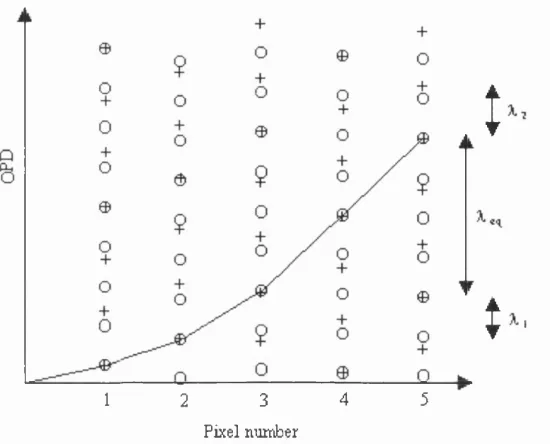
TWPSI is a combined technique o f PSI and two-wavelength interferometry. Figure 1.4 explains the principle o f TWPSI. The ‘+ ’ and ‘o ’ marks are possible OPDs with each wavelength intervals (phase modulo 2n), measured w ith standard PSI technique. The possible solutions at each pixel would be the points at which ‘+ ’ and ‘o ’ marks are overlapped. These possible solutions are spaced with the equivalent wavelength

Since the equivalent wavelength is much longer than each wavelength, the OPD difference between pixels would be less than Xeq/2 and the phase can be correctly unwrapped using standard PSI techniques. The 2n ambiguity o f the measurement using each wavelength can be corrected by using the equivalent wavelength phase data. In this way, the repeatability o f measuring a surface having a sag o f ~ 100 pm was better than 2.5 nm rms (Y. Y. Cheng 1984).

(28)

1 2 3 4 5

I

t

Pixel number

Figure 1.4: O PD construction o f T W PSI technique, reproduced from O ptical Shop

Testing (M alacara 1992). The circles are spaced X\ and the crosses I2.

1 .

2.5 Sub-aperture testing

Sub-aperture testing (O. Y. K w on 1981; S. C. Jensen 1984) is a m eth o d to analyse large optical w avefronts using a set o f sm aller section and pieced together to p rovide the full aperture aberrations. The w avefront departure in each section is w ithin the m easurem ent range o f the instrum ent. A s the later version o f this m ethod, m ultiple annular interferogram s (M A I) (M auro M elozzi 1993) divides the aspheric surface into several overlapping annular sections (rings). E ach section can be teste d w ith the standard PSI, and overlapping o f the sections m akes it possible to stitch them together to give a profile o f the full aperture. It does not require high reso lu tio n o f sensor or sparse-array sensor.

H ow ever, the m ore rings the optics requires to be tested, the w orse the m easu rem en t accuracy is, because o f several sources o f error, e.g. uncertainty in the m easu rem en t o f the radius o f curvature, interferom eter enlargem ent factor, tran slato r m isalig n m en t, ring-to-ring sew ing error, etc (M auro M elozzi 1993). For exam ple, w ere the G em ini secondary m irror tested w ith this m ethod, the num ber o f rings w ould be m ore than 10, since m axim um fringe num ber per pixel is 5 at periphery, as show n in F igure 1.2. T herefore, the accurate m easurem ent cannot be expected w ith this m ethod. It w as suggested in the sam e paper that this m ethod m ight be used in co n ju n ctio n w ith som e sim ple com pensating elem ent to reduce the num ber o f rings, w hich m ig h t bro ad en its applicability to very steep aspheres.

(29)

1.2.6 Alternative method for interferometry

Reviewing the interferometric testing methods developed to overcome the conventional interferometry showed their own advantages and disadvantages. As indicated by Wyant, there is no one solution applicable to all aspheric testing problems. In this situation, the stylus profilometry can be a very effective candidate for the wide application since it has following advantages:

• Since the stylus directly contacts the surface tested and measures the height, it does not require making null correctors, which can reduce the testing cost and eliminate a source o f error.

• It does not require the precise alignment for the measurement.

• It can measure a spheric as well as an aspheric, a rough surface as well as a smooth surface, and a convex surface as easily as a concave surface. Also, it can measure the special shape such as a saddle, which cannot be measured by the null testing. However, the conventional stylus profilometry was also known to have several drawbacks.

• Since the stylus contacts directly the surface and moves along with gravitational force, it can damage the surface.

• The geometrical shape and size o f the tip may distort the profile o f the surface. • When a rough surface is scanned with a low contact force established, the

frequency spectrum o f the vertical motion o f the stylus can overlap the resonance frequencies o f the stylus structure and cause erroneous readings o f the surface profile.

• Two-dimensional profile cannot reveal the whole picture o f the sample.

These disadvantages have been investigated for a long time, and there have been some efforts in reducing these effects. Such activities are explained in chapter 2.

(30)

However, unfortunately, the stylus profilometry applicable to measure the form o f large optics for astronomy was seldom found in the world. Hence, Optical Science Laboratory (OSL) in University College London (UCL) initiated the long-term project in 1992, to develop the stylus profilometry for measuring the large optics very accurately.

1.3 OSL background in developing Profilometry

1.3.1 Testing methods employed in OSL

Since OSL was established in 1984 by Dr. David W alker and Dr. Richard Bingham, it has undertaken numerous projects, particularly in astronomical optical instrumentation, but also in the general area o f optical systems for industry. OSL has a capability o f producing large optics. The 1-metre polishing machine and the 8 ft (2.4 m) diamond milling and polishing machine have been in operation since they were bought from the NEI Parson Ltd in 1987.

With these machines, OSL has tried to have several independent testing methods to eliminate measurement errors that might be generated from applying a method that has some critical errors in its set-up or theory. At present stage, there are three different testing methods employed in OSL: interferometric system, knife-edge test, and profilometric test.

• There are four kinds o f interferometric system in OSL: WYKO 6000, WYKO IR3, shearing interferometer, and scatter plate interferometer. The shearing and scatter plate interferometers (J. M. Burch 1953; Murty 1964) have been used for several years in OSL to test the optics. Their interferograms are captured by CCD camera and analysed using the fringe analysis system, WYKO 4000(WYKO). More advanced fringe analysis systems, WYKO IR3 and WYKO 6000, have been employed in OSL since 1998. WYKO IR3 uses the 00% laser (^=10.6 pm), so that it is very useful in testing aspheric mirrors without any null optics and grinding surface. WYKO 6000 phase shifting interferometer has very high accuracy, which is known to be better than 6 nm. The spheric can be tested by using a supplied reference spherical optics with X/20 quality. Since its performance has been well verified and certified, the performance o f the new technology for measuring optics can be evaluated with respect to this instrument. One disadvantage is that this system requires null correctors to test the aspheric.

(31)

Lateral t

direction Axial

direction

iloggj

□

---B

Figure 1.5: Schematic diagram o f a quantitative knife-edge testing, reproduced by the kind permission o f Kim (Kim 1998).

• The OSL has two types o f knife-edge testing method: conventional knife-edge test and an experimental quantitative knife-edge test. The conventional knife-edge test (Foucault 1858) (Platzeck 1939) determines the form o f mirror qualitatively by a shadow pattern emerging from the knife-edge located on the centre o f curvature. A quantitative knife-edge test was developed by Kim (Kim 1998) in OSL, to enable a quantitative measurement o f the form. It measures the slope o f point on the mirror by using the image at intra and extra focal planes, as can be seen in Figure 1.5. The height distribution o f the mirror is then quantified by the integration o f the slope data. Kim claimed that the Gemini primary mirror, o f which conic constant is - 1.0038, could be measured with this method. Also, he added that the only limitation to measure the aspheric surface came from the limited travel length o f positioners, not from the measurement principle itself. However, this method can not test the convex aspheres without auxiliary optics.

(32)

Stylus Profilometry for Large Optics Testing (SPLOT). Mark 1 and M ark 2 were designed to test the grinding and lapped surface o f which P-V is about ± 4 pm, whereas SPLOT was developed primarily to test the polished surface. The detailed descriptions o f Mark 1 and Mark 2 are shown in the K im ’s thesis (Kim 1993). The brief description o f SPLOT is as follows.

1.3.2 SPLOT

SPLOT was initiated in 1992, with the goal o f testing the polished secondary mirror o f the Gemini telescope. The Gemini telescopes are twin telescopes, which are located at Hawaii and Chile each, so that both north and south hemispheres are covered by the almost identical telescopes. The telescopes are being made by an international partnership o f the U.S.A., U.K., Canada, Chile, Argentina, Brazil, and Australia.

Since the surface figure was required to be less than 100 nm RMS (root-mean-square) (Hansen 1994), very precision profilometry was necessary. A number o f OSL members had been involved in this project. In particular, Hubbard won his Ph.D. degree by taking some steps to new methods in SPLOT.

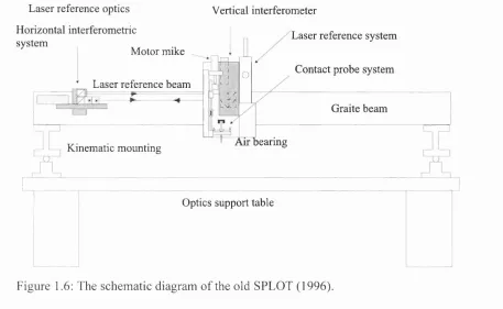
Figure 1.6 is the schematic diagram o f SPLOT in 1996, just when the author joined this project. This consists o f a low-contact force type o f probe system, a laser reference system, and an interferometric distance measuring system. M ost components are loaded on the air bearing carriage, including a vertical slide-way for the probe system, the laser reference system, and the vertical interferometer.

The horizontal interferometer and the beam splitter for generating the reference beam are on a separate Cervit block, which is installed on the granite beam. The reference line is defined by the laser beam that is propagated in the air, not by the granite beam. The position o f the vertical interferometer maintains constant with respect to this reference beam by some feedback system, so that the height o f the surface is measured with respect to this reference line. The probe system is moved down on the target position o f the surface, lifted up after the height measurement and moved to the next position. This gives us two-dimensional profile o f the surface. More details about the system are described in chapter 3.

(33)

Laser reference optics _{Vertical interferometer}

Horizontal interferometric

system Laser reference system

Motor mike _

Contact probe system ^ Laser reference beam

Air bearing Kinematic mounting

Optics support table

Graite beam

Figure 1.6: The schematic diagram o f the old SPLOT (1996).

1.4 Author’s contribution

The author joined this project (SPLOT) on January 1996 as a part o f international collaboration between Korea Advanced Institute of Science and Technology (KAIST) and University College London (UCL). A Ph.D. student in OSL, Hubbard, constructed a prototype of SPLOT and carried out some tests. The author is fully responsible for the development of this project since Hubbard left the project in 1996.

The author has contributed to the project in the following areas:

• Analysis of previous works related to SPLOT, which revealed many sources of error and unreliability and which defined the direction for this thesis.

• Movement of SPLOT to a new metrology room and refurbishment.

• Design and installation of Cervit pillar for the stable reference beam with respect to the tabletop.

• Improvement o f the probe system to increase repeatability and accuracy.

(34)

Development o f a closed loop system for the laser reference system and its performance testing.

Investigation on the sources o f measurement error.

1.5 Summary of the thesis

This thesis details the author’s contribution to the profilometry project (SPLOT). This is a continuing research project at OSL, and as such this thesis does not encompass the entire R&D process. The contents o f the thesis are as follows.

• Chapter 2 introduces the general concepts o f stylus profilometry and application to the large optics testing.

• Chapter 3 describes the principle o f operation o f SPLOT in detail, as it was when the author joined the project (1996).

• Chapter 4 describes the performance test o f the old probe system and development o f new probe system to improve the repeatability and accuracy o f measurement. • Chapter 5 describes the development o f the motorised horizontal drive system. • Chapter 6 describes the development o f the laser reference system based on only

hardware and its performance testing.

• Chapter 7 identifies the sources o f error through the measurements on the nominal flat and checks how accurately SPLOT can measure the aspherics.

• Chapter 8 briefly summarises the results o f this work and suggests future works necessary to meet the ambitious target o f accuracy.

(35)

chapter 2 Stylus Profilometry

2.1 Introduction

The stylus profilometry has been dominant in measuring the profile since the first surface texture recorder was described by Schmaltz in 1929 (Schmaltz 1929). The “Profilometer” was the commercially registered name o f the instrument developed by Ernest Abbott (E. Abbott 1933) in the USA.

In the early stage o f stylus profilometry, several methods were used in order to magnify the vertical movement o f the stylus tip on the surface: light reflection, mechanical lever and optical projector, or simple moving-coil transducer. The information o f the surface was displayed on the photographic paper, smoked glass disc, or the screen o f cathode- ray tube, etc. The vertical magnification in these ways was about maximum 10,000X (Dagnall 1986), which might correspond to 50 nm, supposing that the resolution o f the line displayed be 0.5 mm.

(36)

Electron

Microscope (stereo)

Stylus Profilometry Interferometry Optical heterodyne Profilometry Mireau heterodyne Interferometry Total integrated Scattering 1

(20-1500 A I

(4 A -lOpm)______

I * depends on

(10-2500 A ) instrument

type

(4-1000 A )

(4-3000;A)

(5-350 A rms )

---H Height unresolved

10 100 nm

0.1 10 100

1 10 mm

1000 pm

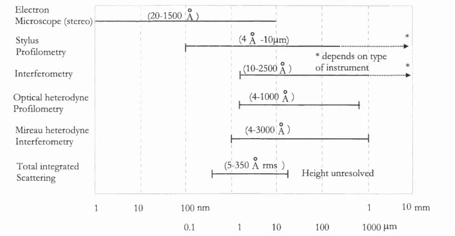
Figure 2.1: The comparison o f the surface profiling techniques in terms o f spatial wavelength range, reproduced from Bennett (Bennett 1985). Numbers in parentheses are the range of heights. The wavelength used in TIS (total integrated scattering) technique is 632.8 nm.

In this chapter, the general structure and principles o f operation of main parts in the stylus profilometry (stylus, transducer, and reference systems) are described in detail. Also, reviewed are aspects of the conventional stylus profilometry that should be modified in order to apply this method to measure the large optics.

2.2 Principle of the Stylus Profilometry

Figure 2.2 is the conceptual diagram of a typical modern stylus profilometry. It mainly consists o f 6 parts: stylus, transducer, traverse unit, reference plane, digitisation circuit, and computer. The stylus directly contacts the surface and is moved across the surface by the traverse unit. The vertical displacement o f the stylus is measured with respect to the reference line. The transducer converts its vertical movements into an electrical signal. This signal is filtered and digitised by the electrical circuit. The microcomputer converts the number into the height information and calculates wanted surface parameters.

(37)

Stylus

Traverse unit

Digitizer

Reference surface

C om puter Transducer

Surface under test

Figure 2.2: The conceptual diagram of a modem stylus profilometry.

Laser

Traversing Interferometer

Carnage Datum

Shaft

Verticm interferometer

Figure 2.3: Schematic diagram o f Form Talysurf traverse unit with the laser interferometric transducer, reproduced from Dagnall (Dagnall 1986).

(38)

2.3 Stylus system

It is not exaggerating to say that the probe system is one o f the most im portant parts in stylus profilometer because it contacts the surface directly and measures the heights o f the contacting point. The properties o f the stylus system are mainly determined by three factors: structure, geometry o f stylus tip (shape and size), and contact force.

2.3.1 Structure

Generally, stylus systems have two generic types o f structure: a pivot (cantilever) system or a plunger system (Leadbeater 1990; Mike Keamy 1998). In a pivot system, an arm supports a stylus tip and the vertical movement o f the tip is detected by the transducer that is attached to the other end o f the arm. A typical structure o f this type can be seen in Figure 2.4. This is a very simple structure and has an advantage in measuring inside o f holes, such as in hollow cylinders. However, due to the dimensions o f its structure (H, Li, and L2 in Figure 2.4), the pivot system generates two

kinds o f non-linear effect, which requires a calibration or compensation process after the measurement:

• The arc motion o f the stylus generates a non-linear variation between the vertical displacement o f the stylus tip (yi) and the value measured by the sensor (yo) (Dobosz 1994), or,

• The arc motion o f the stylus also generates horizontal positional error, which is the difference between the positions o f the stylus tip on the workpiece (x/) and the horizontal position o f the stylus system measured by the sensor (Xo) (Dobosz 1994), or,

= ^ o ~ = A

f

“

[1

“ (To / ^2 Ÿ

I

}“ / ^2

Another disadvantage o f this type is that the measurement range o f the transducer limits the vertical range o f measurement. Even though the long-range transducer such as an interferometric transducer is adopted, the arc motion o f the stylus will move the retro- reflector out o f the beam path, which considerably reduces the vertical measurement range.

(39)

L i L2

H Pivot retro-reflector

or sensor

Figure 2.4: Typical structure o f the pivot type stylus system.

BIAS C O IL S U PE R INVAR R E T R O

R E F L E C T O R H O U SIN G _{AIR BEA RIN G BUSH}SQ U A R E SE C T IO N

Z E R O D U R S P IN D L E

RUBY P R O B E T IP I ^ S E R BEAM

Figure 2.5: I'he typical plunger type stylus system, reproduced from Leadbeater (Leadbeater 1990).

In a plunger system, however, the tip is connected to an actuator or sensor directly without lever so that straight-line motion is possible. It can intrinsically have a larger vertical range than pivot type. Another advantage of this type is that it does not require the compensation process (equation (2.1) and (2.2)), which is necessary in the pivot type. However, it has generally complicated structure, as can be seen in Figure 2.5. This is because it requires the precise mounting for ensuring the straight and frictionless motion of the stylus system and constant and very low contact force. Therefore, it costs much more than the pivot type.

2.3.2 Shape and size of the tip

(40)

the traverse direction o f 2 |am, and 3 |xm in the direction at right angle to the traverse direction, although 0.1 jim width tip is also available. It is mounted so that the direction o f travel is perpendicular to the longer dimension o f the stylus, making it ideal for measuring surfaces having a unidirectional lay such as gratings or single point diamond-machined surfaces (J. M. Bennett 1981).

Many researchers have been investigating the effects o f finite size o f the stylus on the profiling experimentally and theoretically. Bennett (J. M. Bennett 1981) studied the effect o f stylus radius to the diffraction grating (grating space 3.6 p.m) with respect to the lateral resolution, using two different radius o f styli, 8 p.m and 1 pm. The experiment showed that the 8 pm radius stylus gave only a hint o f the grooved nature o f the surface, whereas the 1 pm radius stylus gave nearly complete lateral resolution o f the V-shaped grooves. Bennett derived the condition, with which the feature o f the sinusoidal component is accurately represented as follow:

d > 27r>fhr ,

where r is the stylus radius, d the period and h the amplitude o f the sinusoidal component.

Song et al (J. F. Song 1991) measured the random profile with two different radii tips, 0.5 and 12.5 pm, and found that the peaks and valleys are distorted for the bigger tip. The peaks were wider and the valleys were narrower and shallower and some valleys disappeared from the result, compared to the sharper tip.

Kratz et al (F. ICratz 1996) simulated the effect o f the stylus tip size on the rms roughness measurement and correlation length o f the profile and compared it with the experimental result. It was found that the simulation matches well with the experiment in roughness measurement but some deviations occurred in the correlation length, probably due to the surface-prohe interaction such as friction or distortion by the contact force.

Mendeleyev (Mendeleyev 1997) investigated the effect o f three factors (rms roughness(a) and stylus tip radius (r) and correlation length o f profile (p)) on the rms roughness measurement error, by means o f computer simulation. He found that fractional measuring error ( a = ( a - a ’)/cj where a ’ is the rms roughness o f traced profile) does depend not on individual factors, but on the ratios, a /r and a /p , while a /r were in the range o f 0.005-0.05 and a /p were equal to 0.028 and 0.048. That is, if the ratio a /r is the same, a is the same even though different radius tip is used.

(41)

2.3.3 Contact force

Since the probe is urged to follow the surface by gravity, the contact force always exists. This contact force can sometimes damage the surface. Poon (Chin Y. Poon 1995) demonstrated that even Im g load could damage the glass-ceramic disk substrate if a 0.1 pm radius o f tip was used. A larger radius tip with less load (0.2pm, 0.5 mg) considerably reduced the damage. However, if soft material such as KCl (Mob hardness<2) was measured, this amount o f contact force was found to damage the sample according to Bennett (J. M. Bennett 1981). It was found that 1 pm radius with 0.5 mg load could be used non-destructively on soft material.

Nevertheless, the use o f very low contact force could cause problems in accurate measurement. That is, the system can be affected by the noise generated from roughness surface when measured as well as environmental sources o f vibration. To reduce this effect, Wheeler (Wheeler 1994, US patent N o.5309755) used air damping by inserting a paddle between narrow capacitive sensor plates. This is effective when the overall mass o f the stylus assembly (tip, arm and wire) remains minimal, for example, less than 50 mg.

(42)

2.4 Transducer system

The function o f the transducer is to convert the height variation o f the stylus on the surface into proportionate electrical or digital signal. There are various principles in existence. These may use the change o f electrical properties such as the inductance or capacitance according to the deflection o f stylus tip. Or it may use change o f interference fringe or the change o f resonant frequency in an optical resonator. In this section, the author reviews the performance and the technical characteristics o f transducer systems for highly accurate measurement.

2.4.1 Capacitance and inductance sensors

Capacitance sensors detect the variation o f a capacitor due to displacements o f the electrodes. In normal configurations, this consists o f three electrodes; two outer ones are fixed and the middle one is attached to the stylus. The differential capacitance is varied as the tip is vertically deflected. By arranging the sensors into a capacitance bridge, the differential change in capacitance unbalances the bridge and produces an AC output voltage. If the bridge is driven by a sinusoidal signal with amplitude Vo, the corresponding output is (R. Loxton 1986),

where x is the moving distance from the middle position between outer electrodes. In this way, the accuracy achievable is usually 0.02% o f the travel.

Another way o f using three electrodes is to pick up the electric field potential through the middle electrode (Mike Keamy 1998), instead o f using a capacitance. The outer electrodes are driven by AC signals in which the polarities o f electric field potential are opposite but the amplitudes are the same at the outer electrodes. The middle electrode takes on the electric potential at its location: it produces zero voltage at the middle position between outer plates and drive voltage at maximum deflection. The displacement o f the stylus is measured by demodulating or integrating the voltage measured. Its resolution was not published; however, the target o f this method was set to 0.2 nm (Mike Keamy 1998).

Similar to capacitance sensors, the variation o f inductance has been also used as a transducer system. A ferromagnetic armature is fixed to the other end o f the stylus arm and moves between two coils. The differential inductance is varied as the tip is

(43)

vertically deflected, which unbalances the bridge and generates an output proportional to the deflection. Linear Variable Differential Transformers (LYDT) use this method as well. Its resolution reaches 10 nm over travel bigger than 1 mm, Physik Instrumente (Physik Instrumente GmbH ). The drawbacks are a relatively low frequency response (upper limit o f is approximately 100 Hz) and large non-linearity (D'Arrigo 1996).

2.4.2 Interferometer

Interferometry methods are one o f the most widely used for transducers. Especially, this method is useful in measuring the large distances because o f the coherent properties o f the source (laser). The principle o f distance measurement depends on how fringes are generated. However, irrespective o f the principle, this method requires a quadrature signal to determine the movement direction.

There are two basic approaches to generate fringes: optical path difference and frequency difference. The use o f optical path difference is the conventional method. The retro-reflector is attached to the stylus. As the stylus moves, the optical path length from the beam splitter to the retro-reflector is changed. Then, the distance moved is the fringe number times half-wavelength due to the double path o f the light.

Alternatively, fringes can be generated by the frequency difference o f two beams. This can be accomplished using a grating, so it is called a grating interferometer. It uses the Doppler shift o f the beam frequency. The grating is attached to the stylus in which the motion o f stylus is perpendicular to the line o f grating, which is illuminated by the laser. The diffracted +1 and -1 order beams suffer the Doppler shift due to the motion o f the grating. Since the velocity o f the grating in the direction o f +1 order beam differs from that in the direction o f -1 order beam, there is the frequency difference between two reflected beams as follows (Dobosz 1992),

2v. (2.4)

Av = - g nd

where Vg is the velocity o f the grating, n is the refractive index o f air, and d is the grating constant. The above equation is valid under the assumption that Vg « c .

(44)

2.4.3 Fabry-Perot cavity

A Fabry-Perot cavity can be also used as a precise transducer system, US patent N o.5565987 (Jain Kanti 1996). It consists o f two parallel mirrors, o f which one moves together with the tip. As the tip traverses the surface, it is vertically deflected, and the length o f cavity is changed. Since the resonant frequency o f a Fabry-Perot cavity has a narrow bandwidth, very small deviations o f the cavity can be detected by monitoring the laser beam incident on the cavity. The feedback system modulates the frequency o f the laser beam so that the resonance is maintained. The displacement o f the tip can be measured by monitoring the modulation o f the frequency. A simple calculation shows that 0.5 nm change o f cavity length can be compensated with 5 MHz o f modulation, which is easily obtainable with a commercial acousto-optical frequency modulator.

2.5 The métrologie reference for Profilometry

Measuring the surface height accurately is one key element o f profilometry. Since the height is measured with respect to the reference surface, errors in the reference propagate into errors in the height measurement. Therefore, the reference system is very critical part for the high precision profilometry.

The transducer system must move along a reference line so that the output represents only the stylus movement on the surface being scanned. There are two ways o f generating a reference line: a skid and a separate reference surface (absolute reference surface).

1. A skid is a curved surface, o f which radius is considerably greater than the spacing o f the peaks o f the sample surface. It basically supplies the local flatness and it is well known that it modifies the profile. The effects o f skid-stylus separation on the measurement and skid configurations in several situations are well explained by Whitehouse (Whitehouse 1994).

2. The alternative way is to use a separate reference surface (optical flat), scanned by a second large-radius probe in a fixed relationship to the stylus. A separate reference can be very accurate but limit the scan ranges due to the difficulty o f manufacture and installation o f the large reference with high accuracy.