Predicting Surface Water Critical
Loads at the Catchment Scale
Thesis submitted for the degree of
Doctor of Philosophy
University of London
Martin Kernan
Department of Geography
University College London
ProQuest Number: 10011142
All rights reserved
INFORMATION TO ALL USERS
The quality of this reproduction is dependent upon the quality of the copy submitted.
In the unlikely event that the author did not send a complete manuscript and there are missing pages, these will be noted. Also, if material had to be removed,
a note will indicate the deletion.
uest.
ProQuest 10011142
Published by ProQuest LLC(2016). Copyright of the Dissertation is held by the Author.
All rights reserved.
This work is protected against unauthorized copying under Title 17, United States Code. Microform Edition © ProQuest LLC.
ProQuest LLC
789 East Eisenhower Parkway P.O. Box 1346
Abstract
Current applications of the critical loads concept are geared primarily towards targeting
emission control strategies at a national and international level. In the UK maps of critical
loads for freshwaters are available at 10km^ resolution based on a single representative site
in each grid square. These maps do not take variations of water chemistry within mapping
units into account and are therefore of limited use for application to non-mapped sites. This
thesis describes the development of an empirical statistical model, which uses nationally
available secondary data, to predict freshwater critical loads for catchments lacking the
appropriate water chemistry information.
A calibration exercise using data from 78 catchments throughout Scotland is described.
Water chemistry for each catchment has been determined and each catchment is
characterised according to a number of attributes. Multivariate statistical analysis of these
data shows clear relationships between catchment attributes and water chemistry and
between water chemistry and diatom critical load. The key variables which explain most of
the variation in critical load relate to soil, geology and land use within the catchment. Using
these variables (as predictors) in a regression analysis diatom critical load could be
predicted across a broad gradient of sensitivity = c.0.8). The predictive power of the
model was maintained when different combinations of explanatory variables were used. This
accords the model a degree of flexibility in that model paramaterisation can be geared
towards availability of secondary data.
There are limitations with the model. These relate to the nature of the predictor variables
and the ability of the model to predict critical loads for more sensitive sites. Nevertheless the
ability of the model to differentiate between sensitive and non-sensitive sites offers
considerable scope for environmental managers to undertake national inventories of
Acknowledgements
This research was funded by the Natural Environment Research Council (Grant GT4/92/17/P). Funding for water chemistry analysis was provided by the UGL Graduate School.
I would like to thank my supervisors Tim Allott and Rick Battarbee and co-supervisor Steve Juggins for their advice and encouragement throughout this research.
I was helped on fieldwork by Jon Cox, Chris Curtis and Dave Ryves, each of whom contributed very useful discussion towards many aspects of this thesis.
Analytical water chemistry was carried out at the Freshwater and Fisheries Laboratory, Pitlochry. I am grateful to Ron Harriman for this and for advice in this area. I would also like to thank Tony Osbourne (Dept of Geology, UCL) and Sarah James (Dept of Geology, RHUC) for help with the ion chromatograph and ICP facility respectively.
Much secondary data was made available to me and I am grateful for the co-operation and assistance of the following:
i) The CLAG Freshwaters sub-group for use of the chemistry and other data from the CLAG database.
ii) The Institute of Terrestrial Ecology who provided me with data from the Land Classification and Land Cover datasets. Permission for use of these data was granted by Bob Bunce and Robin Fuller respectively. I am grateful to Jane Hall, Helen Dyke, Jacquie Ullyet and Mike Brown for help with extracting these and other data held at ITE.
ill) ENSIS for permission to use the Acid Waters Monitoring Data and Mike Renshaw who extracted it for me.
iv) The British Geological Society for granting me a license to digitise geology maps.
v) The Macauley Land Use Research Institute for permission to digitise Scottish soil maps and for use of data. I am particularly indebted to Simon Langan for valuable help and advice with extracting and interpreting these data. Mark Hodson, also at MLURI, aided my interpretation of geological data.
I was helped along the steep GIS/Unix learning curve by Dave Allison (from the Remote Sensing Unit at UCL), Trevor Tsang, Su-min Shen and Ian Carson.
For advice on the application of, and dangers associated with, multivariate statistical techniques I am grateful to John Birks.
For help with putting the final product together I would like to thank Catherine Dalton.
Table of contents
A b s tra c t... 2
Acknowledgements... 3
Table of contents ... 4
List of ta b le s... 10
List of fig u re s ... 13
List of appendices... 15
Chapter 1 : Introduction 1.1 Background ... 17
1.2 The critical loads approach ... 18
1.3 Prediction of catchment critical loads - the study ra tionale... 20
1.4 Structure of th e s is ... 21
Chapter 2: Acidification 2.1 Introduction... 23
2.2 Acid r a in ... 24
2.3 Emissions of acidifying compounds ... 25
2.3.1 Sulphur em issions... 26
2.3.1.1 Natural sources ... 26
2.3.1.2 Anthropogenic sources ... 27
2.3.2 Nitrogen emissions... 28
2.3.2.1 Natural sources... 28
2.3.2.2 Anthropogenic sources ... 28
2.3.3 Other emissions ... 29
2.4 Atmospheric transportation and transformation of acidifying com pounds... 30
2.4.1 Dry phase transformation... 30
2.4.2 Aqueous phase transformations... 31
2.5 Atmospheric Deposition... 31
2.5.2 Wet deposition ... 33
2.5.3 Cloud droplet (occult) deposition... 33
2.5.4 Monitoring and mapping deposition p a tte rn s ... 34
2.6 The links between deposition and surface water acidification... 36
2.7 Catchment sensitivity... 37
2.7.1 Geology and s o ils ... 37
2.7.1.1 Introduction ... 37
2.7.1.2 Fundamental concepts - soil acidification... 38
2.7.1.3 Soil as a b u ffe r ... 40
2.7.1.4 Geology as a b u ffe r... 44
2.7.2 Land use and catchment management... 45
2.7.2.1 Conifer afforestation... 45
2.7.2.2 Upland agricultural improvement ... 48
2.7.2.3. Catchment liming ... 48
2.7.2.4. Lake liming ... 49
2.7.3 Catchment morphology and hydrology ... 49
2.7.3.1 Introduction... 49
2.7.3.2 Catchment morphology ... 50
2.1.3.2 Hydrological pathways... 51
2.8 An integrated approach : catchment characteristics as predictors of surface water chemistry . . . 52
2.9 S u m m a ry... 54
Chapter 3: The Critical Loads Concept 3.1 Introduction... 55
3.2 Critical loads for freshwaters ... 55
3.2.1 Diatom critical load ... 57
3.2.2 Henriksen (steady state water chemistry) Critical Load ... 60
3.2.3 The First Order Acidity Balance (FAB) Model ... 62
3.2.4 Dynamic modelling ... 64
3.3. Critical load exceedances... 65
3.5 Problems with mapping resolutions ... 67
3.6 Catchment scale critical loads: a predictive m o d e l... 68
Chapter 4: Research Design and Methodology 4.1 Introduction... 71
4.2 Site selection ... 71
4.3 Temporal variation in water chemistry... 75
4.4 Sampling techniques... 79
4.5 Analytical chemistry... 81
4.6 Secondary data sources ... 82
4.6.1 Phase 1 secondary data ... 83
4.6.1.1 Catchment properties from the CLAG database... 83
4.6.1.2 Soil Critical L o a d s ... 84
4.6.1.3 Land classification data... ... 86
4.6.1.4 Land cover data ... 87
4.6.1.5 Site sensitivity... 88
4.6.2 Phase 2 secondary data ... 90
4.6.2.1 Introduction... 90
4.6.2.2 Catchment delineation... 91
4.6.2.3 Land u s e ... 91
4.6.2.4 Solid geology ... 92
4.6.2.5 Drift deposits... 96
4.6.2.6 S o il... 96
4.6.2.7 Other attributes... 101
4.7 Statistical analysis ... 103
4.7.1 Ordination ... 103
4.7.1.1 Introduction... 103
4.7.1.2 Indirect gradient a n a lysis... 105
4.7.1.3 Direct gradient analysis... ... 106
4.7.1.4 Direct gradient analysis as a data reduction tool ... 108
4.7.3 Multiple regression ... 109
4.8 Discussion ... I l l 4.8.1 Land use d a ta ... I l l 4.8.2 Geology data ... I l l 4.8.3 Soil d a ta ... 112
4.8.4 Deposition d a ta ... 113
Chapter 5: Phase 1 - Preliminary study of model feasibility 5.1 Introduction... 114
5.2 Analysis of the full dataset (954 CLAG sites)... 115
5.2.1 Exploratory data analysis of response variables (water chemistry) ... 115
5.2.1.1 Summary statistics... 116
5.2.1.2 Correlation Structure ... 117
5.2.1.3 Principal Components Analysis ... 119
5.2.2 Exploratory data analysis - explanatory variables ... 127
5.2.2.1 Summary statistics for continuous variables... 127
5.2.2.2 Correlation ... 128
5.2.2.3 Distribution of nominal/ordinal variables... 128
5.2.3 Direct gradient analysis - chemistry and catchment data ... 131
5.2.3.1 Preliminary Redundancy Analysis (RDA) of the nominal/ordinal variables... 131
5.2.3.2 RDA of chemistry and catchment va ria b le s... 132
5.2.3.3 Forward selection of explanatory variables ... 138
5.2.3.4 RDA using DCL as a single response variable... 140
5.3 Analysis of a reduced dataset of more sensitive sites (Ca^'^<20G|ieq I’’ ) ... 144
5.3.1 Redundancy analysis of water chemistry and catchment variables ... 144
5.3.2 Forward selection of environmental variables ... 148
5.3.3 RDA using DCL as a single response variable ... 149
Chapter 6: Phase 2 - Model Development and Calibration
6.1 Introduction... 155
6.2 Exploratory analysis - chemistry and catchment datasets... 157
6.2.1 Water chemistry d a ta ... 157
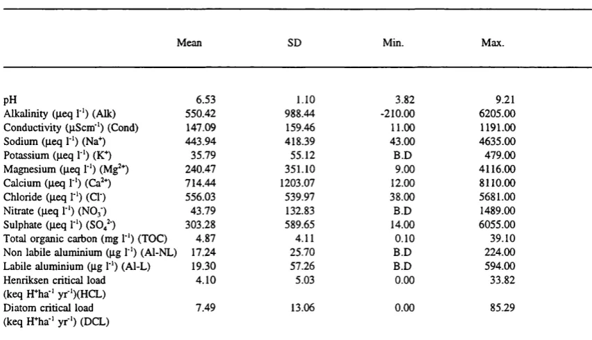
6.2.1.1 Summary statistics... 158
6.2.1.2 Principal components analysis (PCA)- water chemistry d a ta ... 162
6.2.2 Catchment data ... 167
6.2.2.1 Summary statistics ... 168
6.2.2.2 Correlation ... 171
6.2.2.S Principal Component Analysis (PCA) - catchment a ttrib u te s... 174
6.3 Direct gradient analysis - chemistry and catchment variables... 178
6.3.1 Redundancy Analysis (RDA) on full catchment and chemistry datasets... 179
6.3.2 Forward selection of catchment variables ... 184
6.3.3 Redundancy analysis (RDA) using Diatom critical load (DCL) as a single response v a ria b le ... 190
6.3.4 Variance partitioning ... 196
6.4 Analysis of a reduced dataset of more sensitive sites (Ca^*<400|ieq T’ ) ... 203
6.4.1 Exploratory analysis of response (water chemistry) v a ria b le s... 204
6.4.2 Exploratory data analysis - explanatory variables... 209
6.4.3. Direct gradient analysis... 212
6.4.3.1 Redundancy analysis (RDA) on sites where Ca^‘'<400|ieq r ’ ... 212
6.4.3.2 Forward selection of environmental variables... 215
6.4.3.3 RDA using DCL as a single response variable... 218
6.5 S u m m a ry ... 223
Chapter 7: Phase 2 - Model calibration 7.1 Introduction... 226
7.2 Regression results and model diagnostics ... 226
7.3 Multiple Regression with more sensitive sites (Ca^"^<400|ieq I"’) ... 236
Chapter 8: Discussion and Conclusion
8.1 Introduction... 239
8.2 Summary of re s u lts ... 239
8.3 Implications of results for model development... 241
8.4 Methodological Is s u e s ... 242
8.4.1 Sampling s tra te g y ... 243
8.4.2 Water chemistry ... 246
8.4.3 Catchment characterisation ... 247
8.5 Model representation of catchment processes... 254
8.5.1 Geology... 256
8.5.2 Soil... 262
8.5.3 Land use... 276
8.4 Model evaluation... 286
8.7 Further research possibilities... 288
8.7.1 Potential improvements in model paramaterisation... 289
8.7.2 Analysis of catchment data at different spatial resolutions ... 293
8.7.3 Potential for predicting other measures of sensitivity and acid-base s ta tu s ... 294
8.7.4 Model evaluation and further development using national d a ta ... 300
8.8 Implications of model improvement for catchment m anagement... 305
8.9 Conclusions ... 307
References... 310
Appendices ... 332
List of tables
Table 2.1:
Table 2.2:
Table 2.3:
Table 2.4:
Table 4.1:
Table 4.2:
Table 4.3:
Table 4.4:
Table 4.5:
Table 4.6:
Table 4.7:
Table 4.8:
Table 4.9:
Table 4.10:
Table 5.1:
Table 5.2:
Table 5.3:
Table 5.4:
Table 5.5:
Table 5.6:
Estimates of global emissions of sulphur and nitrogen. (From Rodhe et a/.,1995)
Summary of chemical processes in neutralisation of rainfall acidity (from UKAWRG, 1986)
25
43
Soil buffering classes used by Catt (1985, in Hornung, 1990b) to map soil neutralising capacity in Wales. Terminology based on classification
by Avery (1980) 43
Buffering capacities of solid geology in Wales (from Hornung at a i, 1990b) 45
Precision, accuracy and detection limits of analytical methods, Freshwater
Fisheries Laboratory (FFL) 81
Mineralogical and petrological classification of soil material and critical loads of soils (after Nilsson and Grennfelt, 1988 and Sverdrup and Warfvinge,
1988 - modified by Hornung at ai, 1994) 85
Number of sites in each land classification class 86
Aggregated land cover classification (9 classes) 88
Aggregated land cover classification (6 classes) 88
Surface water sensitivity classes as defined by soil and geology classes
(after Hornung at ai, 1995a) 90
Categories adopted for classification of the solid geology map (1:625,000) of the UK according to sensitivity to acidification (after Kinniburgh
and Edmunds, 1984) 94
Classification of individual map units of the solid geology map (1:625,000) of the UK according to sensitivity to acidification (after Kinniburgh
and Edmunds, 1994) 94
Soil series sensitivity classes (after Hornung at ai, 1995a) 99
Weathering rates for 17 major soil associations (after
Langan et a/., 1995) 101
Summary statistics for untransformed chemistry/response variables
(n = 954) 117
Matrix of Pearson product-moment correlations for 14 transformed water
chemistry determinands from 954 CLAG sites 118
Results of PCA on transformed water chemistry determinands (954 sites). 121
Ca^* and DCL values for seven sites along the first PCA axis 125
Key chemical values for selected outlying sites (t=|ieq l'\ *=p,Scm \
BD=Below detection limits) 126
Summary statistics for untransformed catchment/explanatory variables
Table 5.7:
Table 5.8:
Table 5.9:
Table 5.10a:
Table 5.10b:
Table 5.11:
Table 5.12:
Table 5.13:
Table 5.14a:
Table 5.14b:
Table 5.15:
Table 5.16:
Table 6.1:
Table 6.2:
Table 6.3:
Table 6.4:
Table 6.5
Table 6.6:
Table 6.7:
Table 6.8a:
Table 6.8b:
Table 6.9:
Table 6.10:
Table 6.11:
Table 6.12:
Table 6.13:
Table 6.14:
Matrix of Pearson product-moment correlations between transformed catcfiment
attributes for 954 CLAG sites 128
RDA of chemistry and selected classifications 132
Results of RDA on chemistry and environmental variables (954 sites) 134
Forward selection of environmental variables 139
RDA summary using variables identified in the forward selection procedure 139
Results of an RDA on DCL and catchment attributes (954 sites) 141
Forward selection with DCL as a sole response variable 141
Results of RDA on chemistry and environmental variables (469 sites) 145
Forward selection of environmental variables 148
RDA summary using variables from forward selection 148
Results of an RDA on DCL and catchment attributes (459 sites) 149
Forward selection with DCL as a sole response variable 150
Summary statistics for untransformed chemistry/response variables in the
Phase 2 (calibration) dataset (n=78) 158
Results of PCA on transformed water chemistry determinands (n = 78) 163
Summary statistics for untransformed catchment/predictor variables (n=78) 169
Matrix of Pearson product-moment correlations for 31 transformed catchment variables (n = 78)
Results of a PCA on transformed catchment attributes (see Table 6.3 for full description of variables)
Values for dominant catchment variables for 5 sites along PCA Axis 1
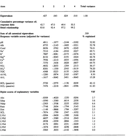
Results of RDA on chemistry and catchment variables {n=78)
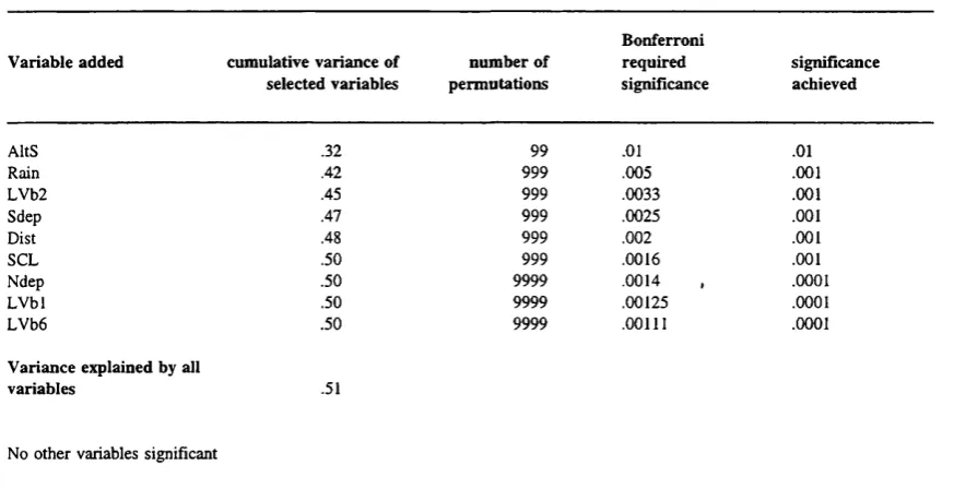
Catchment variables identified by the forward selection procedure
RDA summary using catchment variables identified by forward selection
Results of an RDA on DCL and catchment attributes
Forward selection with DCL as a sole response variable
Redundancy Analyses on Catchment Variable Components
Results of (partial) RDA (A=Soil, B=Geology, C=Land use, D=Extrinsic, AnBnc=Unique covariance between A,B and C)
Results of PCA on transformed water chemistry determinands for sites where Ca^^ <= 400peq T’
Results of a PCA on transformed catchment attributes on sites with Ca^+ < 400eq I''
Table 6.15: Results of RDA on chemistry and environmental variables for sites
where Ca^‘'<400neq T’ 213
Table 6.16a: Forward selection of catchment variables at sites where Ca^‘'<400^eq T’ 217
Table 6.16b: RDA summary using variables from forward selection at sites where
Ca^+<400|ieq I'' 217
Table 6.17: Results of an RDA on DCL and catchment attributes (using forward
selection) for sites where Ca^'" < 400p,eq 1-1 219
Table 6.18: Redundancy Analysis (with forward selection) on datasets of varying
sensitivity 221
Table 7.1: Multiple linear regression output with G1, G2, SOL, and LC2 as
predictors. 228
Table 7.2: Multiple linear regression output with G1, G2, hF and LG2 as predictors 232
Table 7.3: Multiple linear regression output with G1, G2, and LC2 as predictors 233
Table 7.4: Results of regression analyses on a variety of catchment attribute
combinations 234
Table 7.5: Multiple linear regression output with SCL3 and LC2 as predictors
List of figures
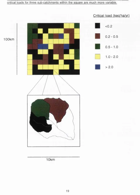
Figure 1.1; Schematic illustration showing critical load variation 19
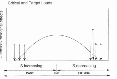
Figure 3.1: Critical and target loads concept (after Battarbee et al., 1994). The critical load for a site is exceeded at (a)\ (b) and (c) are critical loads for specific species. A target load (T) can be chosen to protect selected species as acid deposition declines in the future.
Full recovery is represented by point (a) on the ’future’ curve. 56
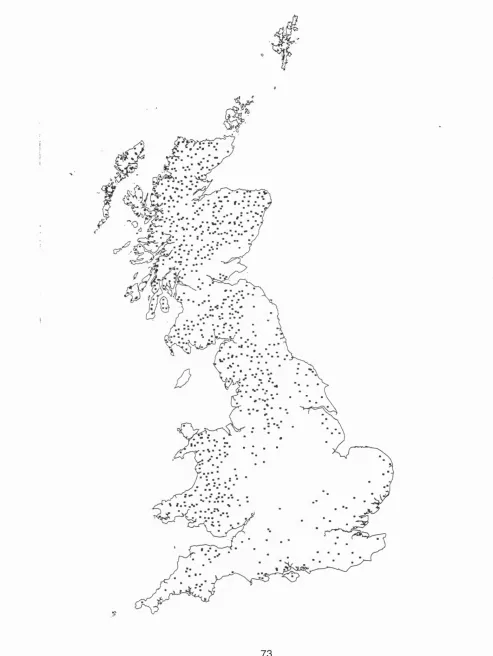
Figure 4.1: Location of CLAG sites used in Phase 1 analysis 73
Figure 4.2: Location of Phase 2 model calibration sites 76
Figure 4.3: Calcium concentrations at minimum, mean and maximum flow for 11
Acid Waters Monitoring Network sites 78
Figure 4.4: Flow diagram illustrating the soil variables available for characterising
catchments 102
Figure 5.1: PCA correlation biplot of 15 water chemistry determinands for 954 CLAG sites
(plotted using CALIBRATE - Juggins and ter Braak, 1993) 122
Figure 5.2: PCA biplot showing the position of sites relative to the first two PCA axes
(vectors have been multiplied by three for clarity) 124
Figure 5.3: Scatterplot of DCL against PCA axis 1 site scores 126
Figure 5.4: Bar charts showing the distribution of sites for the nominal/ordinal
explanatory variables 129
Figure 5.5: RDA correlation biplot of chemistry and surrogate catchment data (954 sites) showing water chemistry (solid vectors), continuous catchment parameters
(dashed vectors) and dummy variables (filled circles) 137
Figure 5.6: Box plots showing DCL values classed according to nominal explanatory
variables 142
Figure 5.7 Scatterplots showing DCL against continuous catchment variables 143
Figure 5.8: RDA biplot of chemistry and environmental data (469 sites) 147
Figure 5.9: Box and whisker plots of distribution of site DCL according to classification
variables - sensitive sites 150
Figure 5.10: Scatterplot showing DCL against continuous environmental variables
-sensitive sites 151
Figure 6.1: Percentage of Diatom Critical Load classes for the Phase 1, Phase 2 and
CLAG mapping datasets (Curtis at al, 1995) 161
Figure 6.2: PCA correlation biplot of Phase 2 water chemistry (plotted using CALIBRATE -Juggins and ter Braak, 1993) - vectors have been multiplied by three to aid
clarity 165
Figure 6.3: Scatterplot of DCL against PCA Axis 1 site scores 167
Figure 6.4: PCA correlation biplot of Phase 2 water chemistry (plotted using CALIBRATE -Juggins and Ter Braak, 1993) - vectors have been multiplied by three for
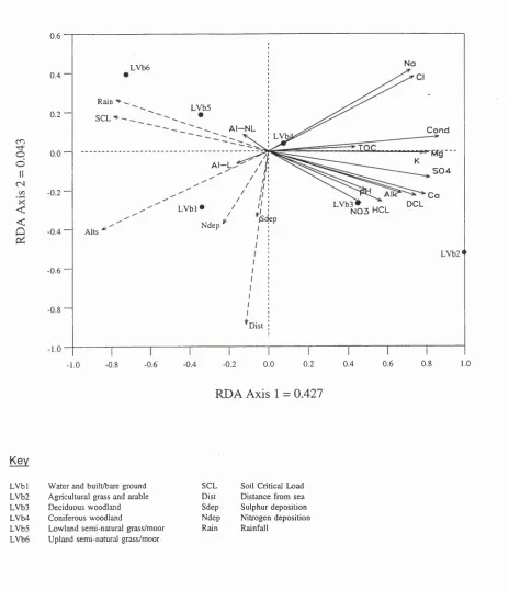
Figure 6.5: RDA biplot of chemistry and catchment data showing water chemistry (solid vectors) and catchment attributes (dashed vectors). See Tables 6.1
(chemistry) and 6.3 (catchments) for key 183
Figure 6.6: RDA biplot of chemistry and catchment data showing water chemistry (solid vectors) and catchment parameters (dashed vectors) for soil map unit,
the latter included following forward selection. 186
Figure 6.7 Scatterplots showing DCL against variables selected by the forward selection
procedure 194
Figure 6.8: Schematic representation of the explanatory variable components and covariances used in (partial) RDA on significant catchment variables and DCL. ATIB is the unique covariation between A and B, AFlBIlC between A, B and C etc., 200
Figure 6.9: Bar chart showing the results of (partial) RDA on catchment attributes and
DCL 202
Figure 6.10: PCA plot of water chemistry determinands from sites where
Ca^+ <=400peq r' 207
Figure 6.11: Scatterplot of Diatom Critical Load (DCL) against PCA Axes scores for sites
where Ca^<400peq T’ 208
Figure 6.12: PCA correlation biplot of transformed catchment attributes on sites where
Ca^"<400peq I'' 211
Figure 6.13: RDA biplot of chemistry and chemistry attributes for sites where
Ca^^<400peq I ’ 214
Figure 6.14: RDA biplot using variables from forward selection at sites where
Ca^"<400peq r' 218
Figure 6.15: Scatterplots showing diatom critical load against variables selected by
forward selection procedure (sites where Ca<400peq 1'^) 220
Figure 7.1: Residuals plotted against predicted DCL 229
Figure 7.2: Distribution analyses of studentized residuals 230
List of appendices
4.1; Sampling strategy originally adopted during Phase 2 332
4.2: Phase 2 site locations 339
4.3: Scatterplots of calcium concentration (peq 1-1) against
flow (cumecs) for selected Acid Waters Monitoring Network sites 343
4.4: Water chemistry for Phase 2 sites (including critical load
values) 349
4.5a: Summary of ITE Land classification system (from
Bunce et al., 1982) 352
4.5b: Hierarchical aggregations of ITE Land classification system
(from Bunce et a!., 1982), aggregated using TWINSPAN (Hill, 1979) 357
4.6: Classes from the Land Cover Map of Great Britain. Correspondence
between the 25 'target' cover types and 17 'key' cover types
(from Fuller and Groom, 1993a) 359
4.7: Percentage of each land cover class at each site (25m resolution,
6 class aggregation) 361
4.8: Percentage of each sensitivity class for geology in each
catchment 363
4.9: Percentage of each drift type in each catchment 365
4.10: Phase 2 catchment values for each soil variable 366
4.11 : Miscellaneous data for Phase 2 catchments 369
5.1 : Summary statistics for transformed chemistry/ response variables 371
5.2: Summary statistics for transformed catchment/explanatory variables 372
6.1: Pearson product-moment correlations for 16 transformed water chemistry
determinands (full dataset, n = 78). 381
6.2: Comparative analysis of alternative sub-sets of the catchment data 383
6.3: Summary statistics for untransformed water chemistry variables
(sensitive subset) 392
6.4: Matrix of Pearson product-moment correiations for 16 transformed
water chemistry determinands (sensitive subset, n = 46). 393
6.5: Summary statistics for untransformed catchment attributes
-sites where Ca^* <=400peq 1'^ 394
6.6: Matrix of Pearson product-moment correlations for 28 transformed
catchment attributes (sensitive subset, n = 46) SCL2 not present
CHAPTER 1 : INTRODUCTION
1.1 Background
The deposition of anthropogenicaiiy derived acidic precipitation onto terrestrial and aquatic
ecosystems is now generally recognised as a major environmental problem, particularly over
large areas of North America and Europe (Beamish and Harvey, 1972; Gjessing etal., 1976;
Thompson et al., 1980; Wright et a!., 1980; Cowling, 1982). The consequences for aquatic
ecosystems are well documented (Harriman and Morrison, 1982; Ormerod and Wade, 1990;
Muniz, 1991; Gorham, 1992; Havas and Rosseland, 1995). In response to this, a number
of international protocols have been signed seeking to limit and ultimately reduce the
emissions of acidifying compounds. In 1985 the sulphur protocol was signed by most
UNECE member states. This aimed to reduce national emissions of SOg by at least 30%
by 1993, based on levels in 1980. The subsequent EG Large Combustion Plant directive
(LCPD) requires an emission reduction of 60% from large combustion plants by 2003, also
based on a 1980 start year. This further stipulates that UK LCPD NO^ emissions be reduced
by 30% by 1998.
This kind of emission control strategy employs a blanket reduction approach. Clearly,
however, reductions need to be targeted at those countries where emissions are greater.
In addition, the amount of damage to ecosystems varies from region to region, as does the
potential for further damage. Consequently, to optimise reductions so that they are reduced
where most needed, these spatial variations need to be considered. Those areas with low
neutralising capacities are more susceptible to acidification than well buffered areas. Such
considerations led to the development and adoption of the critical loads approach in Europe
1.2 The critical loads approach
The most commonly used general definition of critical loads is that proposed by Nilsson and
Grennfelt:
"the highest deposition of acidifying compounds that will not cause chemical changes leading
to long term harmful effects on ecosystem structure and function".
The development of the critical loads approach has been widely reviewed (e.g. Henriksen
etal., 1990; Bull, 1991; Brodin and Kuylenstierna, 1992; Kàmâri, eta!., 1992a; CLAG 1994;
UN EGE, 1994; Bull, 1995). The critical loads approach for freshwaters has resulted in the
production of national (CLAG, 1994) and international maps (Hettelingh et a!., 1991;
Downing etal., 1993; Posch etal., 1995) of critical loads values. Mapped data for deposition
of acidifying compounds used in conjunction with the critical loads maps provide a picture
of areas where critical loads are exceeded. Future deposition scenarios can be used to
assess the effects of emission reduction strategies. The approach has now been
incorporated into the second Sulphur Protocol, signed in 1994, which recommended
emission reductions both on the basis of environmental effects and the cost of control
strategies (UN ECE, 1994). In the UK, critical loads are now used as part of pollution control
policy (HMSO, 1990).
The European and UK mapping exercises are very much geared towards targeting emission
control strategies at regional, national and international levels. The UK freshwater critical
loads maps show critical loads for sulphur and where these have been exceeded throughout
the UK (CLAG, 1994). These are mapped in a grid form at lOkm^ resolution. However the
the critical load value for each square is not necessarily representative of the sensitivity of
Figure 1.1: S chem atic illustration showing critical load variation with m apping resolution. A lthough the 10km sguare exem plified has a m apped critical load of <0.2keg ha'^ y r '\ the critical loads for three sub-catchm ents within the sguare are much more variable.
Critical load (kea'ha/vr)
100km
<0.2
n
1 0 - 2 . 0
10km
maps at this resolution, using a grid based approach, are of limited use for management and
assessment of specific catchments. Thus although the national critical loads map for the UK
is used by the Forestry Authority to identify where afforestation by trees might lead to
freshwater acidification, it is acknowledged that the map cannot be used to determine the
susceptibility of surface waters in individual catchments (Forestry Authority, 1993). The
critical loads approach, as currently applied, is inappropriate where catchment scale
assessments are necessary. In an applied context these are required by forestry
organisations (e.g. Forest Authority), conservation bodies (e.g. Countryside Commission for
Wales, Scottish Natural Heritage, English Nature) and pollution control organisations (e.g.
Environment Agency) to examine ecosystem response to changing land use and changing
industrial emission patterns, and to assess the likely consequences on catchment organisms
of increased acid deposition. In addition, understanding and prediction of the ecosystem
responses to anthropogenic acid loading is best approached at a catchment scale where
well defined boundaries enable assessment of the interactions between terrestrial and
aquatic systems to be made (Hornung et al., 1990a). As a consequence, there is a need
for an approach where the sensitivity of specific catchments can be gauged.
1.3 Prediction of catchment criticai loads - the study rationaie
Currently assessments of surface water critical loads can only be achieved by an analysis
of water chemistry. However, water chemistry data are not readily available at a national
level and, where the sensitivity of a large number of catchments across a wide geographical
area needs to be assessed, the only existing approach is to undertake costly water sampling
programmes. Data relating to catchment characteristics (e.g. soil, geology, land use) are
more commonly mapped and are available nationally. Given the integrated nature of the
terrestrial and aquatic systems within catchments it is likely the characteristics of the former
The overall aim of this thesis is to examine the character of the reiationships between
catchment attributes and surface water chemistry and to assess whether these can be used
to develop an empirically based model which will predict critical loads from quantified
catchment characteristics. In an applied context, it is hoped that the use of nationally
available catchment data to calibrate the predictive model will enable critical loads for
surface waters to be predicted for any site throughout the UK.
1.4 Structure of thesis
Chapter 2 introduces the concepts and processes of surface water acidification. It comprises
an integrated examination of the atmospheric emission of acidifying compounds, the transfer
and transformation of these compounds, deposition, chemicai reactions in the soil/vegetation
environment and the geochemical and hydrological processes operating between the soil
and surface water spheres. Within this context previous attempts at relating catchment
characteristics to aspects of surface water chemistry are examined. This chapter shows how
processes operating within the catchment dictate surface water chemistry and thus
determine sensitivity. The predictive model is based on the strength of these relationships.
The background, development and current issues relating to critical loads are reviewed in
Chapter 3. The use of modelling, at a variety of scales, to predict freshwater critical load is
introduced and discussed with regard to the requirements of catchment scale applications.
The methodology used to develop the predictive model is described in Chapter 4. The
origins and derivation of the data used to represent catchment characteristics are presented
together with the statistical techniques employed in model calibration. Chapter 5 presents
the results of a preliminary analysis of secondary water chemistry and a variety of surrogate
catchment characteristics. Multivariate statistical techniques are used to assess the feasibility
developed in Chapter 6 where a calibration water chemistry dataset is used in tandem with
catchment specific data to identify catchment variables which most explain variation in,
initially, water chemistry as a whole and, subsequently, critical load. Chapter 7 describes a
series of multiple regression analyses which use these key catchment variables as
predictors of freshwater critical loads.
Discussion in Chapter 8 initially focuses on the limitations and uncertainties of the predictive
model. A number of suggestions for improving model utility are presented. The value of the
model as a tool for catchment management is discussed both in its present form, and
CHAPTER 2 : ACIDIFICATION
2.1 Introduction
This chapter examines the processes which are responsible for the acidification of surface
waters and how these relate to the physical systems within which they operate. These
processes begin with the emission of acidifying compounds of sulphur (S) and nitrogen (N)
into the atmosphere from a wide variety of sources. Chemical transformation in the
atmosphere alters the nature of these compounds prior to deposition. Once deposited as dry
or aqueous media the compounds are subsequently modified, to varying degrees, by
interaction with vegetation, soil and geology and, via a variety of hydrological pathways,
reach streams and standing water bodies within the catchment. After introducing the
atmospheric processes which result in elevated acidity levels in precipitation, the primary
objective of this chapter is to examine the catchment processes which occur at the interface
between water and soil, geology and vegetation. The hypothesis here is that these
processes, because they are involved in modifying the chemical composition of incoming
precipitation, ultimately determine the chemistry of catchment surface waters. The factors
or attributes which most influence catchment sensitivity to surface water acidification will
need to be represented in a predictive model. More emphasis is placed on the role of
sulphur cycling within the catchment rather than nitrogen cycling because the model is
calibrated for critical loads for sulphur (see Section 3.6). Leaching of N species also leads
to acidification (or eutrophication). However the processes governing N cycling are much
more complex than 8 because the former is also involved in many biological reactions.
These processes are discussed more fully elsewhere (e.g. Gunderson and Bashkin, 1994;
2.2 Acid rain
’Acid rain’ as a physical phenomenon is not a recent, nor anthropogenicaiiy induced,
development. If pH values less than 7 are to describe acidity then rain is always acidic. At
equilibrium, unpolluted rain has a pH of approximately 5.67 (Kennedy 1992) a result of
naturally occurring acids and bases and atmospheric reactions, mainly with carbon dioxide
(COg) which forms carbonic acid (HgCOg). This is, in effect, a theoretical value as rain can
be contaminated by wind blown alkaline dusts which raise pH and by sulphur and nitrogen
from volcanic and biological sources which can lower it. Background pH values of 4.0 to 6.0
have been recorded in remote areas of the Southern Hemisphere (Galloway et al., 1982)
and it has been suggested that rainfall pH at pristine sites varies between 4.5 to 5.6 as a
result of temporal and spatial variations in the sulphur cycle (Charleson and Rodhe, 1982).
This range is proposed as the probable background level of acidity that would have
characterised the precipitation of pre-industrial Europe (Galloway at a!., 1982; Irwin and
Williams, 1988).
The term ’acid rain’ as used to describe rain polluted by anthropogenic means was first used
in connection with air pollution and its effect on the buildings and vegetation of urban
England following observations that rain approaching Manchester was found to contain
sulphuric acid proportional to its distance from the town (Smith, 1852). Subsequent research
contended that acid rain over the Lake District stemmed from air masses that were acidified
as they passed over the industrial regions to the south and east and that the deposition of
large amounts of sulphuric acid over a period of a hundred years had probably initiated
significant ecological changes in the bog pools and upland tarns of the region (Gorham,
1958). Ten years later it was argued that ’acid rain’ was acidifying lakes and killing fish in
Sweden and that the origins of this polluted precipitation were the heavily industrialised parts
Britain were responsible for acidified precipitation were largely ignored throughout the
1970’s. It was not until the 1980’s that the concept of long range trans-boundary air pollution
became widely accepted and import/export balances between countries of acidifying
pollutants such as sulphur dioxide (SO^ and nitrogen oxides (NOJ are now calculated on
an annual basis (Iversen et al., 1991 in Lovblad et al., 1992).
2.3 Emissions of acidifying compounds
Elevated acid levels in precipitation stem primarily from the emission of compounds of
sulphur and nitrogen oxides as well as ammonia (NH3) (Rodhe et al., 1995) although there
are a variety of other contributors including hydrochloric acid and volatile organic compounds
(Irwin and Williams, 1988). Table 2.1 summarises current estimates of global emissions of
S and N compounds.
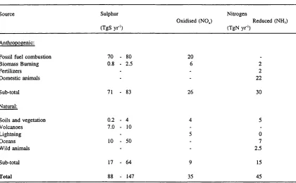
Table 2.1: Estimates of global emissions of sulphur and nitrogen. (From Rodhe eta!., 1995)
Source Sulphur
(TgS yr-')
Oxidised (NO,)
Nitrogen
Reduced (NH,) (TgN y r ‘)
Anthropogenic:
Fossil fuel combustion 70 - 80 20 .
Biomass Burning 0.8 - 2.5 6 2
Fertilizers - - 2
Domestic animals - - 22
Sub-total 71 - 83 26 30
Natural:
Soils and vegetation 0.2 - 4 4 5
Volcanoes 7.0 - 10 -
-Lightning - 5 0
Oceans 10 - 50 - 7
Wild animals - - 2.5
Sub-total 17 - 64 9 15
2.3.1 Sulphur emissions
2.3.1.1 Natural sources
Natural sources of atmospheric sulphur are derived, in order of importance, from biogenic
sources, sea-spray and geothermal activity. Sulphates derived from sea-spray do not directly
contribute to acid deposition as they occur in neutralized form (Rodhe etal., 1995) and need
not be considered here. It should be noted however that ion exchange processes,
specifically Na^ displacing acidic and AP^, can depress the pH of runoff water following
precipitation inputs with high concentrations of marine salts (Langan, 1989; Harriman etal.,
1995a).
The most important natural source of atmospheric sulphur is the biological reduction of
sulphur compounds (Cullis and Hirschler, 1980). These are generated by the non-specific
reduction of sulphur in marine algae, soils and decaying vegetation (Rassmussen, 1974) and
by bacteria specifically reducing certain sulphur compounds (Hallberg et a!., 1976). It is
thought that the principal sulphur compound emitted biogenically is hydrogen sulphide (Cullis
and Hirschler 1980). However, the importance of organic sulphur compounds such as
dimethyl sulphide (DMS) and carbon disulphide, derived from organic sulphur in algae,
plants and animals as well as inorganic sulphate, has also been noted (Davison and Hewitt,
1992; Liss et a!., 1994; Tarrasson et a!., 1995) and it is argued that this is the primary
mechanism for the natural transmission of biogenic sulphur to the atmosphere (Rassmussen,
1974).
The overwhelming contribution to geothermal emissions is from volcanic eruptions which
produce significant amounts of sulphur dioxide and hydrogen sulphide (Kellog etal., 1972).
found to occur (Cullis and Hirschler, 1980; Rampino and Self, 1982), sulphur bearing
compounds have a limited residence time in the atmosphere (Charleson and Rodhe, 1982)
and the acidifying effect of a volcanic eruption is liable to have a strong, short-lived local
bias (e.g. Letter and Birks, 1993).
2.3.1.2 Anthropogenic sources
The magnitude of anthropogenic emissions of sulphur has increased markedly over the past
century although the contributions from coal and petroleum combustion, petroleum refining
and the smelting of non-ferrous ores have changed relative to each other to a considerable
degree (Cullis and Hirschler, 1980).
The most abundant source of anthropogenically derived atmospheric sulphur remains the
combustion of coal and its by-products (Galloway, 1995). A substantial amount of the coal
used industrially and domestically contains over 2% sulphur, about half of which is present
as iron pyrite (FeSg), the remainder being organic (Kennedy, 1982). Sulphur dioxide is
readily produced when these elements are burned, for example;
4FeS2 + 1 1O2 = > 2 Fe203 + 8 SO 2 (2 .1)
Petroleum products also contribute significantly to elevated levels of atmospheric sulphur.
Despite the fact that petrol consumption has expanded more rapidly than that of coal, levels
of sulphur emission have increased less rapidly than the total consumption of petrol (Cullis
and Hirschler 1980). Both recovery and desulphurisation processes have become more
efficient.
increase in sulphur emissions by adopting energy conservation policies and employing
desulphurisation technology. This, together with greater emphasis on gas as a fuel and a
decline in heavy industry has been reflected in a stabilisation of emissions. In fact,
anthropogenic sulphur emissions have declined in Europe and North America over the past
decade (Hultberg etal., 1995) although increases have been observed in Asia, particularly
China (Rodhe at a!., 1995).
2.3.2 Nitrogen emissions
Nitrous oxide (NOJ emissions (comprising both nitric oxide (NO) and nitrogen dioxide (NOg))
have a dual role in acid deposition. They are crucially involved in the photochemical
production of ozone and OH radicals, important factors in the atmospheric reactions leading
to acidification of precipitation and, more directly, as precursors of acidity (Irwin and Williams
1988). While, in the atmosphere, reduced N in the form of ammonia (NHg) neutralizes nitric
(HNOg) and sulphuric acid (HgSOJ (ApSimon etal., 1987). However, NH^ (NHg + N H / from
dry and wet deposition respectively) also has the capacity to cause acidification in
ecosystems (Van Breeman et al., 1982).
2.3.2.1 Natural sources
The primary sources of natural NO^ and NHg emissions are essentially those involving
ecosystem losses through dissimilation and denitrification. These include biomass burning,
ammonia oxidation, microbial activity and marine photolytic and biological processes. Other
sources of NG^ include lightning production and stratospheric input (Irwin, 1989).
The combustion of fossil fuels constitutes the main source of anthropogenic NO^. This is
derived both from the nitrogen held in the fuel and from the oxidation of atmospheric
nitrogen. As a consequence NO^ emission is dependent on the combustion processes as
well as the properties of the fuel, making quantification more difficult than SOg emissions.
A significant proportion of the NO^ produced in this way stems from motor vehicle exhaust
(Williams, 1987) which has increased substantially since the 1940’s both absolutely and
relative to other sources of NO^.
A second major source of anthropogenically derived NO^ emissions is biomass burning for
agricultural land clearance. Biomass burning also accounts for a significant amount of NHg
emissions although these are dominated by livestock wastes and fertilizer application (see
Table 2.1). Other minor sources include traffic exhaust, soil microbial activity, coal
combustion and human respiration (ApSimon al et al., 1987; Buijsman at a/.,1987).
Emissions of NHg have increased recently as a result of more intensive animal husbandry
(ApSimon etal., 1987).
Spatially, the global distribution of anthropogenic NO^ emissions are broadly comparable
with those of SOg, with high concentrations in Europe and North America. However, the
recent decreases in SOg emissions have not been mirrored by a decline in NO^ (Irwin,
1989). Approximately 90% of global NHg emissions originate in Asia where food production
contributes a higher proportion of N emissions than fossil fuel consumption (Galloway,
1995).
2.3.3 Other emissions
Volatile organic compounds (VOCs) are comprised of reactive hydrocarbons and
virtue of their involvement in the generation of oxidizing radicals (Inwin, 1989). VOC
emissions are extremely difficult to quantify as they arise from sources other than
combustion and agricultural activity, including evaporation and certain industrial and
commercial processes (Irwin and Williams, 1988).
2.4 Atmospheric transportation and transformation of acidifying compounds
When emitted from terrestrial and oceanic sources S is typically in an oxidised state. Both
oxidised and reduced N are common. These pollutants typically remain in the atmosphere
for only a few days before they are deposited. During that time SOg and NG^ may be
transported for hundreds of kilometres and undergo certain physical or chemical
transformations (UKRGAR, 1990). The chemical fluxes which characterise transformation
between the original compound and that which is ultimately deposited will vary according to
whether the compounds are subject to dry or aqueous transformations. The most important
interactions tend to be those with the oxidising species (particularly OH radicals) and NHg.
2.4.1 Dry phase transformation
In the gas phase, oxidation of S requires reactions primarily with the OH radical although
under certain pH conditions ozone and hydrogen peroxide (HgOg) become important
oxidising agents (Penkett etal., 1979). During gas phase transformations NOg will compete
with SO4 for OH radicals and the former will tend to oxidise preferentially . The reactions
between the OH radical and oxides of S and N produce HgSO^ and HNO3 respectively, both
strong acids but with substantially different dry deposition velocities (Irwin and Williams,
1988).
very rapidly. Ammonium nitrate aerosols are formed either by the scavenging of HNO3 by
coarse particles (sea salt based in maritime air and alkaline soil particles in continental air)
or by the reaction of HNO3 with ammonia producing fine particles (Den/vent, 1987). The dry
deposition rates of these aerosols are likely to be fairly low and as a consequence they have
a relatively long residence time. The production rates of nitrate aerosol and nitric acid are
an important controlling mechanism in determining the balance between residence times
(and thus transportation distances) of sulphur and nitrogen in the atmosphere.
2.4.2 Aqueous phase transformations
SOg oxidises in rain and cloud phases, primarily through reactions with ozone (O3) and HgOg
(Penkett et al., 1979). The relative importance of these oxidising agents remains unclear.
Reactions with O3 are limited by ozone solubility and pH while HgOg is highly soluble and not
dependent on pH. Oxidation of SOg in the aqueous phase is of great importance and may
account for up to 70% of sulphate in precipitation (Scire and Venkatram, 1985). During
winter when photochemical activity, and thus OH concentration is low, it has been suggested
that such processes are the only means of oxidising SOg (Clark at al., 1984). There is no
significant aqueous phase transformation mechanism in the production of nitric acid.
The removal of both sulphur and nitrogen species in the aqueous phase involves scavenging
of both gaseous species and particulate aerosols (Irwin and Williams, 1988). With regard to
the former, SOg removal is limited by the poor solubility in water although aqueous phase
oxidations can increase the SOg removed from the gas phase.
2.5 Atmospheric Deposition
aquatic systems. These are termed dry deposition, wet deposition (through precipitation) and
cloud droplet deposition (droplet impaction onto vegetation surfaces).
2.5.1 Dry deposition
The dry deposition of gases and particulates involves a transfer from the boundary layer to
the vicinity of the surface, molecular diffusion and uptake at the surface by dissolution,
sorption or chemical reactions (Reynolds and Ormerod, 1993). Untransformed oxides are
deposited by adsorption and absorption while transformed gases fallout onto ground and
vegetation surfaces. These gases include HNO3, HCI and NHg. The rate of uptake is
governed by conditions at three levels. Above and within the forest canopy, deposition is
dependent on windspeed and the aerodynamic roughness of the vegetation surface. Tilled
soil, moorland and forestry are characterised by increasing surface roughness. At the
vegetation/atmosphere interface and within the stomata, rates of uptake are controlled by
molecular diffusion. At leaf surfaces uptake is governed either by chemical reactions
occurring between the leaf surface and the gas or by entry into the leaf via stomata pores
and subsequently by solution in the intercellular fluid. The dominant control over deposition
rates will depend on the reactivity of the gas deposited (Fowler et al., 1989). Other factors
can influence the uptake pathways of individual gases. At night uptake of SOg and NOg
takes place via chemical reactions on the surface of the leaf whereas, during the day, when
stomata pores are open, the uptake occurs through the pores and subsequently, in solution
in intercellular fluids (Fowler and Cape, 1985). The control here is stomatal opening which
is determined by changes in temperature and light. Surface wetness is also a factor which
influences chemical reactions on the leaf surface although, for many vegetation types, dry
deposition of SOg to wetted surfaces is not appreciably greater than uptake on dry surfaces
2.5.2 Wet deposition
Wet deposition comprises the atmospheric acids (and bases) which are deposited onto
terrestrial and aquatic ecosystems via precipitation. This can occur, for example, when
H2SO4 is incorporated into water droplets or ice crystals and falls to the ground as
precipitation (rainout). Alternatively, if in particulate form, H^SO^ or HNO3 can be removed
from the atmosphere by raindrop impaction (washout). This includes the seeder feeder effect
(Bader and Roach, 1977) which involves the scavenging of sulphuric and nitric acid held in
mist or low lying orographic cloud formed as part of frontal weather systems by precipitation
from overlying clouds (Bergeron, 1965). This tends to increase ionic deposition in cloud-
capped upland areas. The feeder cap cloud is generally characterised by higher
concentrations of acidic species than the precipitation from the seeder cloud above
(Carruthers and Choularton, 1984). The lower mountain cloud caps incorporate the higher
concentrations of ions in the atmospheric boundary layer whereas in the frontal clouds the
processes of raindrop formation are initiated by the vapour growth of snowflakes. This does
not efficiently incorporate the dissolved particulate cloud droplets and, as the snowflakes
melt at lower altitudes, raindrops are formed which scavenge cloud droplets in the feeder
cloud as a result of collision coalescence. Frontal weather systems are responsible for much
of the precipitation over upland areas (Fowler etal., 1995) as the moist boundary layer rises
over elevated terrain. Thus the seeder-feeder effect is primarily responsible for deposition
of acidifying compounds in these areas, a supposition supported by experimental work
(Fowler at a!., 1988; Dore et a!., 1992; Inglis et a!., 1995).
2.5.3 Crowd droplet (occult) deposition
Exposed vegetation in upland areas can directly intercept water droplets held in wind driven
than in rainfall in the same area (Crossley etal., 1992) and it is suggested that cloud droplet
deposition in areas prone to low cloud could increase wet deposition estimates by up to 2 0 %
above that detected in rainfall gauges (Dollard et a!., 1993). Deposition loadings vary with
different vegetation communities (Ferrier etal., 1990). Estimates of wet and bulk deposition
should thus be modified to account for direct impaction in upland areas.
2.5.4 Monitoring and mapping deposition patterns
Measuring dry deposition presents particular difficulties as it tends to be governed by surface
properties and a wide variety of measurement techniques have been developed for this
purpose (Ross and Lindberg, 1994). Dry deposition rates of SOg onto vegetation and soil
for different surfaces throughout Great Britain have been calculated (Garland, 1978; Fowler
and Unsworth, 1979; Fowler and Cape, 1985). Rates are calculated from the product of
near surface concentration and an appropriate deposition velocity. This is inversely related
to the distance from the source. As a consequence, dry deposition tends to be greatest near
major emission source areas and contributes more than 75% of total deposition in Southern
and Eastern England (Cottrill et al., 1986). Estimated annual inputs of acidity from dry
deposition of SOg have been mapped showing that dry deposition in the industrial Midlands
and north of England is much greater than wet deposition while the converse is true in
western Wales and north Scotland (Fowler and Cape, 1985).
Wet deposition can be measured relatively easily by collecting precipitation and multiplying
the amount by solute concentrations. This precipitation weighting technique enables spatial
and temporal patterns to be identified. In spatial terms two aspects of wet deposition require
consideration, the concentration in precipitation of acidifying compounds and the amount of
acidity actually deposited (Irwin and Williams, 1988). UK Maps showing the concentration
difference (Cottrill et al., 1987). The greatest concentrations are found in the east of Britain
where rainfall levels are lower while deposition is much greater in areas of higher rainfall in
North West England and North Wales. The relative contributions of HgSO^ and HNO3 in the
UK have been estimated as 71% and 29% respectively (Fowler etal., 1982) although the
latter is becoming increasingly important both in absolute terms (Skeffington and Wilson,
1988) and relative to the former (Galloway and Likens 1981, Rodhe and Rood, 1986). The
relative contribution of each to soil and water acidification is less easy to quantify due to the
mitigating effects that ecosystem interactions have on N species (Sutton and Fowler, 1992).
The concentration of acidic species in precipitation also exhibits seasonal variation with non
marine sulphate and nitrate maxima generally occurring in the spring or early summer (Irwin
and Williams, 1981). Variations in composition can also occur between and within
precipitation events (Coscio etal., 1982). At one site in Eastern England 30% of the annual
sulphate deposition occurred in five days (UKAWRG, 1986) while in Wales 30% of deposited
acidity falls on less than 5% of wet days (Reynolds, 1987). The implications for ecosystem
response of pulsed deposition episodes are discussed below.
In general terms non marine sulphate (/.e that not derived from sea spray) and nitrate have
fairly similar spatial patterns with lower concentrations in the north and west while those in
the East Midlands and East Anglia are up to a factor of 10 greater (Campbell et al., 1987).
For dry deposition, UK maps are not based on a monitoring network because of the
difficulties involved in obtaining accurate measurements. Estimates are based on semi-
empirical mathematical models which incorporate transport, transformation and removal
processes (Barrett and InArin, 1983). Maps are produced on a 20km^ grid basis using the
proportions of different land types in each square (UKRGAR, 1990). On a European scale
1995). National maps are based more on measurement networks. In the UK, wet deposition
maps for S and N are based on a network of 38 monitoring sites together with the UK
Meteorological Office precipitation measurement network (Fowler et al., 1994). Maps have
been produced which incorporate the effects of orographic enhancement (UKRGAR, 1990;
Dore et a!., 1992). A modelling approach to deposition mapping has also been developed.
Initially, the Harwell Trajectory Model (HIM) coupled SOg, NO^, NHg and HCI with simple
meteorology data (DenA/ent et a!., 1988; Metcalfe et a!., 1989). The Hull Acid Rain Model
(HARM) refines this approach although it presently concentrates on modelling 8 deposition
(both at current emission levels and under future emission scenarios). Using data on
emissions, rainfall, windspeed, trajectories, dry deposition and wet removal the HARM model
produces similar deposition patterns as those using measured data (Metcalfe and Whyatt,
1994)
It is has been shown that there is considerable variation in deposition levels onto different
landscape features and at different elevations. This variation is not fully incorporated into
maps at 2 0 km^ scale and precludes the use of these maps for identifying deposition at the
catchment scale. This has important implications for the application of the critical loads
approach at this scale where it is necessary to compare the sensitivity of the surface waters
for a specific catchment with the actual deposition loading to identify where critical load
exceedance may occur (Erisman, et a!., 1995). Acid loading onto individual catchments is
dependent on altitude, slope, aspect, vegetation cover and location, factors which can vary
substantially from catchment to catchment, even at a local scale (Ross and Lindberg, 1994).
The significance of these uncertainties on the development and application of a catchment
scale predictive model are discussed further in Chapters 3 and 8 .
Although the link between elevated levels of anthropogenically derived acid deposition and
the acidification of poorly buffered soils (Reuss and Johnson, 1986; Tamm and Hallbacken,
1988; Reuss and Walthall, 1990) and freshwaters (Oden, 1968, Battarbee et a i, 1985,
Henriksen et a i, 1988) is now almost universally accepted, it has been the subject of some
debate. The occurrence of acid waters in areas of acid soils has been seen as reason to
refute the acid deposition explanation in favour of one based solely on changes in the
terrestrial ecosystem (Rosenqvist, 1978; Krug and Frink, 1983). However there is strong
empirical evidence linking acid deposition to freshwater acidification (Reuss et a i, 1987).
The use of palaeolimnological techniques has been particularly prominent in this respect
(Battarbee, 1990; Battarbee et al., 1988, Patrick and Stevenson 1990, Fritz et a i, 1990).
This is corroborated by the results of dynamic modelling used to reconstruct historical trends
in acidification (Whitehead et a i, 1990). The role of organic acids, occurring naturally in the
soil, as precursors has also been recognised (Seip et a i, 1990).
On the basis of these studies it is assumed here that recent (post 1800 A.D.) surface water
acidification is primarily a result of acid deposition. Whether deposition leads to acidified
waters in individual catchments will depend on the level of buffering within the catchment
{ie., the catchment sensitivity). The attributes which are likely to determine sensitivity relate
to the soil, geology, hydrology and vegetation characterising the catchment.
2.7 Catchment sensitivity
2.7.1 Geology and soils
2.7.1.1 Introduction
requires a recognition of the natural processes of soil development and acidification. The
chemistry of the soil determines the chemistry of the soil solution and thus the chemical
composition of surface water. The effect of anthropogenically derived acid precipitation on
the soil system and its relationship with vegetation is addressed here. Emphasis is placed
on soil as a buffer for acidic input, particularly the complex interrelationships between soil,
geology and surface water.
2.7.1.2 Fundamental concepts - soil acidification
The response of soil to increased inputs of acidic species is determined by soil chemistry.
Of crucial importance in this respect is the cation-exchange complex. This comprises
negative charges on clay minerals or soil organic matter (Reuss and Johnson, 1986). The
negatively charged exchange complex is dominated by base cations in alkaline or neutral
soils, aluminium species in acid mineral soils and in acid organic soils. Soil acidity is
therefore determined by the relative amounts of base cations and acid aluminium species
on the exchange complex. Acidification can occur when the number of negative charges
increases relative to base cations. This may result from an increased organic matter
accumulation or clay formation, or the removal of base cations by leaching. Conversely, an
increase in base cations relative to negative charges will increase alkalinity. Base cations
may be added via atmospheric deposition or from the weathering of soil minerals and a
reduction in negative charges can result, for example, from biomass burning.
Soil acidification can be quantified in a number of ways although it cannot be measured
using any single index (Reuss and Johnson, 1986). Soil pH can be used to define
acidification status although difficulties arise over the physical meaning of this concept and
its dynamic nature over time (Reynolds and Ormerod, 1993). An alternative measure is