A Fusion Link Prediction Method Based on Limit Theorem

Article

1

A Fusion Link Prediction Method Based on Limit

2

Theorem

3

Yiteng Wu *, Hongtao Yu*, Ruiyang Huang, Yingle Li and Senjie Lin

4

National Digital Switching System Engineering and Technological R&D Center, Zhengzhou 450002, China

5

* Correspondence: [email protected] (Y.W.); [email protected] (H.Y.); Tel.: +86-150-9348-9229

6

Abstract: The theoretical limit of link prediction is a fundamental problem in this field. Taking the

7

network structure as object to research this problem is the mainstream method. This paper

8

proposes a new viewpoint that link prediction methods can be divided into single or combination

9

methods, based on the way they derive the similarity matrix, and investigates whether there a

10

theoretical limit exists for combination methods. We propose and prove necessary and sufficient

11

conditions for the combination method to reach the theoretical limit. The limit theorem reveals the

12

essence of combination method that is to estimate probability density functions of existing links

13

and nonexistent links. Based on limit theorem, a new combination method, theoretical limit fusion

14

(TLF) method, is proposed. Simulations and experiments on real networks demonstrated that TLF

15

method can achieve higher prediction accuracy.

16

Keywords: link prediction; combination method; theoretical limit; TLF method

17

18

1. Introduction

19

Limit theory is a basic theoretical issue and has attracted wide interest across many fields. On

20

the 100th _{anniversary of its foundation, Science raised 125 unresolved scientific questions, and many}

21

of these issues related to limit theory [1]. Link prediction predicts missing links in current networks

22

and new or dissolution links in future networks [2]. With continuous improvement of link

23

prediction methods and, the theoretical limit of link prediction has attracted considerable research

24

interest [3].

25

Considering structure or attribute features, link prediction methods based on classification have

26

been proposed by computer science community [4]. Subsequently, more insightful methods of

27

network structure, such as similarity based methods, have become a focus, these methods pay more

28

attention to the physical meaning. At the same time, similarity index fusion methods are springing

29

up [5,6]. Recent years, with the development of deep learning, some deep features extraction

30

methods have been proposed [7,8], the fusion of structure and attribute information has been

31

attached importance again [9]. These methods have strong consistency. We divide link prediction

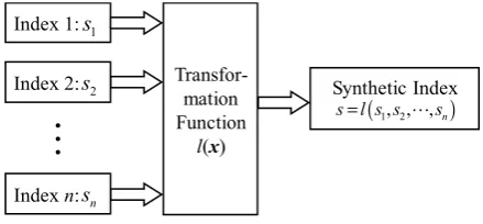
32

method into single and combination methods, based on whether they use multidimension

33

information, and whether they define the relation of multidimension information directly. For

34

example, single methods, such as RA index [10], which defines the relation of common neighbors

35

and degree of nodes directly; and classification based methods, index fusion methods, fusion of

36

structure and attribute information methods belong to link prediction combination methods.

37

Most combination methods perform better than single methods, and are robust to many

38

network types. However, what is the reason for this improved accuracy and robustness, and is there

39

a theoretical limit for combination methods? This paper proposes the mathematic description of

40

combination methods, and obtains the necessary and sufficient conditions for theoretical limit. The

41

limit theorem also has important practical application value. It reveals the ultimate goal of

42

combination methods that is to estimate probability density functions of existing links and

43

nonexistent links. Thus, an appropriate form of the transformation function could be selected from

44

the complete set. Based on limit theorem, a new combination method, theoretical limit fusion (TLF)

45

method, is proposed. We use Parzen kernel method [11] of destiny estimation in the TLF method.

46

Simulations and empirical studies have shown that TLF method can achieve higher prediction

47

accuracy.

48

Section 2 introduces a mathematical description for the theoretical limit of combination

49

methods and evaluation metrics for link prediction. Section 3 proposes and proves necessary and

50

sufficient conditions for the theoretical limit of combination methods. Section 4 proposes a fusion

51

link prediction method based on limit theorem (TLF method). Section 5 provides simulation

52

examples for limit theorem and proposed TLF method with other combination methods, and gives

53

comparison experiments in real networks. Section 6 and 7 discuss some results and conclude the

54

paper.

55

2. Problem Description and Evaluation Metrics

56

2.1. Problem description

57

Given a network G V E( , ) at time t, where V =

{

v v1, , ,2 vN

}

is the set of nodes and

58

{

1, , ,2 M

}

E= e e e is the set of links. The observed links, E, are randomly divided into training, ET ,

59

and probe, EP , sets, where E E= TEP and ETEP = ∅. Link prediction aims to predict

60

missing links at current network or new links for a future time t t'( '>t)[2]. Link prediction

61

combination methods fuse several similarity indices and obtain a synthetic index and can be

62

described in mathematic as follows. Let ( ₁, ₂, , )T n

X X X

=

X  be the scores of existing links as given

63

by n structural similarity indices, and follow probability density function (pdf)f( )x =f x x( , , , )1 2xn .

64

LetY=( , ,Y Y_{1 2} , )Y_n Tbe the scores of nonexistent links as n structural similarity indices, and follow

65

1 2

( ) ( , , , )n

g x =g x x  x . We need to find the transformation function, l( )x , and obtain the synthetic

66

score, X =l( )X , Y l= ( )Y that maximizes evaluation metrics. Figure 1 is the diagram of

67

combination methods.

68

Index 1:



Transfor-mation Function

l(x)

Synthetic Index

1

s

Index 2:s₂

Index n:s_n

(1, , ,2 n)

s l s s= s

Figure 1. Combination methods

2.2. Evaluation metrics

69

Let the synthetic score X =l( )X follow pdf f xX( ), and Y l= ( )Y follow g xY( ). X and Y are

70

independent. We have the following metrics.

71

2.2.1. Area under the receiver operation characteristics curve (AUC)

72

A receiver operating characteristics (ROC) curve is a two-dimensional depiction of classifier

73

performance [12]. In the field of link prediction, the ROC curve abscissa represents the probability

74

of nonexistent links i.e., the false positive rate (FPR), when the link prediction score is greater than

75

some threshold,

μ

, andFPR=μ∞g x dxY( ) . The ordinate represents the probability of missing links,

76

i.e., the true positive rate (TPR), when score >

μ

, and TPR=_μ∞f x dx_X( ) , TPR is equivalent to Recall.

77

According to [13], AUC can be derived as

(

)

( ) ( ) ( )

1 1

( ) ( ) 1 ( ) ( )

2 2

1 1

sgn( ) ( ) ( )

2 2

1

sgn 1 , 2

X Y

X Y

X Y X Y

X Y X Y

X Y

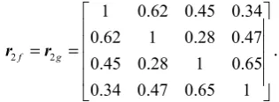
P X Y f x g y dxdy

f x g y dxdy f x g y dxdy

x y f x g y dxdy

X Y >

> ≤

> =

 

= +  − 

 

= − +

= _ − + _











(1)

where

79

1, 0 sgn( ) 0, 0

1, 0 x

x x

x >

 

= =

_{− <} 

. (2)

In the real network, original data is randomly divided into training set and the probe set. Eq. (1)

80

means that for n independent comparisons, if there are n’ comparisons where the missing link

81

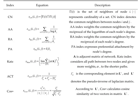
returns a higher score and n’’ comparisons where the missing and nonexistent links return the same

82

score, we can obtain the algorithm expression of AUC:

83

' 0.5 ''

AUC n n

n

+

= . (3)

2.2.2. Precision

84

Precision can be defined as the ratio of correct to (correct and error) prediction proportions

85

when score >μ , i.e.,

86

1

1 2

1

1 2

( ) ( )

Precision

( ) ( ) ( ) ( )

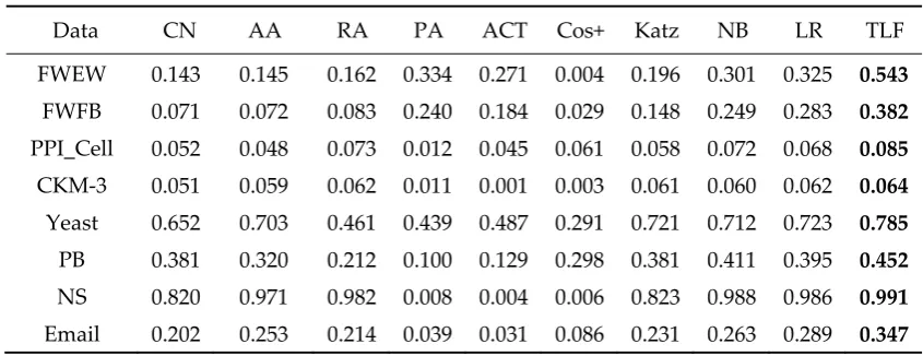
( )TPR . ( )TPR ( )FPR

X

X Y

P f x dx

P f x dx P g x dx

P

P P

μ

μ μ

ω

ω ω

ω

ω ω

+∞

+∞ +∞

=

+

=

+







(4)

In the real network, if the top L links are predicted ones, with m links being right (i.e., there are

87

m links in EP_{), then}

88

Precision m L

= . (5)

Owing to the imbalance of positive and negative samples, link prediction usually uses AUC

89

metric. In application, high Precision means target links are accurate, and these links can be used

90

directly. AUC and Precision are two important metrics in link prediction, we will study the

91

theoretical limit using the two metrics.

92

3. Theoretical Limit Theorem

93

Theorem. Let ( ₁, ₂, , )T

n

X X X

=

X  and ( ,_{1 2}, , )T

n

Y Y Y

=

Y  be random vectors following the joint

94

distributions f( )x and g( )x , respectively, where m{ : ( ) ( )x f x g x =C g, ( ) 0,x ≠ ∀ ∈C } 0= . (m

95

represents the measure of a set.) Then the following conditions are equivalent.

96

(a) A monotonically increasing function r x( ) exists, such that l( )x =r f[ ( ) ( )], ( ) 0x g x g x ≠ ，a.e.

97

n ∈

x .

98

(b) Transformation function l( )x produces maximum AUC.

99

If we add a condition in Theorem that prior probability of existing and nonexistent links be P( )ω1 and

100

2

( )

Pω , respectively. Then the following conditions are equivalent to (a) and (b):

(c) for any α , there exists the corresponding threshold μl for transformation l( )x , and satisfies

102

1 2

( ) _l X( ) ( ) _l Y( )

P _μ f x dx P _μ g x dx

α ₌ ω _+∞ ₊ ω _+∞ _{, such that transformation function l( )x produces}

103

maximum Precision.

104

Proof. (a)(b):

105

From the equivalent definition, AUC maximum is the maximum area under the ROC curve. For

106

any FPR, if the TPRs corresponding to the ROC curve reach maximum, then the AUC reaches the

107

maximum, i.e.,

108

( ( ) )

FPR Y( ) ( )

E l

g x dx g d

μ μ

∞

>

=



=



x x x, (6)

( ( ) )

TPR _X( ) ( )

E l

f x dx f d

μ μ

+∞

>

=



=



x x x, (7)

where E l

(

( )x >μ

)

is a set

{

x∈n: μ∈, ( )l x >μ

}

, and m

{

x: ( )l x =C, ∀ ∈C 

}

=0.

109

We use Lagrange’s undetermined multipliers to solve this problem. For any specified FPR

110

(denoted as FPR0), the TPR corresponding to the ROC curve reaches maximum is equivalent as ϕ

111

reaches maximum,

112

[

]

0

( ( ) ) ( ( ) )

0 _{( ( ) )}

( ) FPR ( )

FPR ( ) ( ) .

E l E l

E l

f d g d

f g d

μ μ

μ

ϕ λ

λ λ

> >

>

 

= + _ − _

= + −







x x

x

x x x x

x x x (8)

Function ϕ will be maximized if we choose set E l( ( )x >μ) such that the integrand is

113

positive, i.e., if

114

( ) ( ) 0

f x −λg x > , (9)

then x∈E l( ( )x >μ). Which means, no matter what is λ, if we select the set of x which

115

makes the integrand f( )x −λg( )x always be positive, the function ϕ will reach maximum; if the

116

set contains x that makes the integrand be negative, function ϕ will decrease. Let

117

( ) ( ) ( )

l x = f x g x and μ λ= , and the set, E l( ( )x >μ), equals toE f( ( ) / ( )x g x >λ), which satisfies

118

(8), i.e.

119

[

]

0 _{( ( )/ ( ) )}

FPR ( ) ( )

E f g λ f g d

ϕ λ= +



_{x x>} x −λ x x. ₍₁₀₎

Thus, for any FPR, the TPR corresponding to the ROC curve reaches the maximum, so the AUC

120

reaches the maximum when X and Y are transformed by l( )x = f( ) ( )x g x .

121

Let r x( ) be a monotonically increasing function; and h x( )be the inverse function of r x( ). If

122

'( ) 1 '( )

h x = r x , then h x( ) and r x( ) have the same monotonicity, and both are increasing functions.

123

Thus, | '( ) |h x =h x'( ). The pdf of X₂ =r X( ₁) is fX₂( )x = f h x h xX₁[ ( )] '( ), and the pdf of Y2=r Y( )1 is

124

2( ) 1[ ( )] '( )

Y Y

g x =g h x h x . Thus,

125

(

)

(

)

2 2

1 1

1 1

2 2

1 1

AUC ( ) ( ) ( )

( ) '( ) ( ) '( ) ( ) ( )

( ).

x

X Y

x

X Y

x

X Y

P X Y f x g y dydx

f h x h x g h y h y dydx

f x g y dydx

P X Y

+∞

−∞ −∞ +∞

−∞ −∞

+∞

−∞ −∞

= > =

=

=

= >













(11)

We have proved (a)(b).

126

(b)(a): If l2( )x ≠r l[ ( )]x , where r x( ) is increasing function, there exists l2( )x such that

127

,

X Ytransforming from l2( )x can also produce maximum AUC, and then the corresponding ROC

128

curves are the same. Otherwise, if ROC curves are different, except the same part, for any FPR, there

129

is at least a ROC curve which doesn’t reach maximum TPR, and contradict with maximum AUC.

130

Since m{ : ( ) ( )x f x g x =C, g( ) 0,x ≠ ∀ ∈C } 0= and the ROC curve is the same for any point

131

(FPR,TPR) on the two ROC curves, thus,

i. For any FPR [0,1]∈ , and any μFPR , there exist μ2 FPR , such that E l( ( )x >

μ

FPR)

133

2 2FPR

( ( ) )

E l

μ

= x > for a.e. x∈n;

134

ii. For any μFPR* >μFPR, if

* FPR

( ( ) )

E l x >μ *

2 2FPR

( ( ) )

E l μ

= x > and E l( ( )x >μFPR)=E l( ( )2 x >μ2FPR), then

135

*

2FPR 2FPR

μ >μ .

136

Let y1=l( )x , then a set of y1 exist with nonzero measure, such that l2( )x ≠r l[ ( )]x , i.e.,

137

1 2

{ : ( ) [ ( )]} 0

m y l x ≠r l x ≠ . Let _{σ =}{y l₁: ( )₂ x _≠r l[ ( )]}x . If y₁∈σ , l2( ), ( )x l1 x satisfies function

138

relation l2( )x =s l[ ( )]x , but s x( ) is not increasing, then for any μ σ1∈ , condition (ii) does not hold.

139

If y1∈σ , l2( )x and l( )x are not functionally related, then neither condition (i) or (ii) hold. Thus

140

(b)(a) is established.

141

(c)⇔(b): Let k=TPR FPR be the slope of the secant for any point on the ROC curve to the

142

origin, then Precision=k k( +λ λ), =P( )ω2 P( )ω1 . For any α , that l( )x produces maximum

143

Precision is equivalent that k reaches maximum. And equivalent that for any α , α=

144

1 2

( ) _l X( ) ( ) _l Y( )

Pω _μ+∞ f x dx P₊ ω _μ+∞g x dx_{, TPR ( )} l f x dxX μ

+∞

= is maximum. Since this condition is established

145

for any α , then it is equivalent that for any FPR [0,1]∈ , the corresponding TPR reaches maximum,

146

and equivalent to l( )x produces maximum AUC.

147

4. A fusion link prediction method based on limit theorem

148

The limit theorem of combination method shows that when selecting transformation function

149

as l( )x = f( ) / ( )x g x or its monotone increasing transformation, the AUC and Precision of synthetic

150

score reaches the maximum. In the real network, because f( )x and g( )x are unknown, the pdfs

151

need to be estimated from multidimensional data. Let the estimated pdfs be fˆ( )x and gˆ( )x . On

152

the basis of limit theorem, we define the transformation function as the ratio of estimated pdfs, i.e.,

153

ˆ_{( )} ˆ_{( ) / ( )ˆ}

l x = f x g x . (12)

Then we obtained the synthetic score, s l=ˆ( )x , and used for link prediction. This method is called

154

theoretical limit fusion (TLF) method.

155

Before evaluating f( )x and g( )x , the input link prediction scores need to be normalized,

156

2 *

1 1

0.5 ( , )

( , ) , 1, 2, ,

( , )

k

k N N

k

i j

N s i j

s i j k n

s i j = =

⋅

= =

 

 . (13)

( , )

k

s i j represents the k-th similarity score for node pair i j, . N is the dimension of adjacent matrix,

157

and n is the number of similarity indices.

158

The limit theorem of combination method transformed the link prediction indices fusion

159

problem into the estimation of pdfs. Statistical methods for estimating density functions can be

160

applied to this problem, directly. Parzen kernel method [11] of destiny estimation is used in this

161

paper. The multivariate kernel density estimate defined as:

162

(

)

1

1 1

ˆ ( ) _d n _i

i

f K

h nh ₌

 

= _ − _

 



x x x , (14)

where h is the window width, and K

( )

x is a multivariate kernel defined for d-dimensional x,

163

such that

164

( )

1

dK d =



 x x . (15)

A form of the pdf estimate commonly used is Gauss kernel,

165

( )

( )

/ 2

1 exp

2 2

T

d K

π

₋ 

=  

 

x x

x . ₍₁₆₎

In summary, the steps of TLF are listed as Table 1.

166

Table 1. The steps of TLF method.

168

Step 1 Divide the network into training set, ET_{, and probe set, E}P_;

Step 2 According to Eq. (13), normalize these similarity indices, then we distinguish existing links and nonexistent links in the training set;

Step 3

Based on Eq. (14), estimate the pdfs of existing links and nonexistent links, and

we obtain the estimated pdfs as fˆ( )x and gˆ( )x ;

Step 4 Obtain the synthetic score of n structure similarity indices according to Eq. (12); Step 5 Calculate the accuracy such as AUC metric or Precision metric on the probe set.

5. Simulation and experiment

169

5.1. Simulation examples

170

Four types of structural similarity indices were simulated to evaluate node pairs with and

171

without links. The pdfs of the structural similarity indices are also provided. We construct 3 groups

172

of known distributions for the similarity indices pdfs. One thousand samples extracted from

173

10000 existing links and 100000 samples of nonexistent links were generated following the

174

appropriate pdfs. The 1000 samples serve as probe set; the 100000 samples with 1000 probe links

175

serve as unknown links for training; and the (10000 1000)− samples serve as train set of existing

176

links. Each sample had 4 dimensions to simulate 4 similarity scores. We first compute AUC and

177

Precision for each dimension, then use proposed TLF method to obtain the synthetic score and

178

calculate the AUC and Precision, compared with other combination methods such as Naïve Bayes

179

and logistic regression. Finally, we calculate AUC and Precision using the theoretical limit theorem

180

and compare with the above methods.

181

Let random vectors X=(X X1, 2,X3,X4)T and Y=( ,Y Y Y Y1 2, ,3 4)T be the scores of existing and

182

nonexistent links, which follow f( )x = f x x( , , , )1 2 xn and g( )x =g x x( , , , )1 2  xn pdfs,

183

respectively.

184

Let f( ), ( )x g x are 4-dimensional normal distributions,

185

(

)

1

(

)

1/2 / 2

1 1

( ) exp

2 (2 )

T p

f

π

−

 

= − − − 

 Σ 

Σ

x x μ x μ , (17)

where diag

( )

Σ 1=

(

_{σ σ σ σ1}2, ₂2, ₃2, ₄2

)

T, and Σij =rijσ σi j.

186

The parameter sets for the 2 groups of simulation examples are as follows.

187

Group 1: Θ =1f {μ1f,Σ1f}, and Θ =1g {μ1g,Σ1g};

188

Group 2: Θ =2f {μ2f,Σ2f} and Θ =2g {μ2g,Σ2g}.

189

In each group, 1 (1, 2,1.7, 2.1)

T f =

μ ，₁ (1.3,2.5,2.1,2.8)T g =

μ , 2 (1, 2,1.7, 2.1)

T f =

μ , 2 (1.5,3.5, 2.8,3)

T g =

μ ,

190

( )

(

2 2 2 2

)

1

diag Σ _f 1= 1.5 , 2.2 ,3 , 2.5 T , diag

( )

1

(

2 , 2.2 ,3 , 2.52 2 2 2

)

T

g =

Σ 1 , diag

( )

2

(

1.5 , 2.2 ,3 , 2.52 2 2 2

)

T f =

Σ 1 ,

191

( )

(

2 2 2 2

)

2

diag Σ_g 1₌ 2.5 ,3.5 , 4 , 2.5 T,

192

1 1

1 0.8 0.76 0.56 0.8 1 0.85 0.74 0.76 0.85 1 0.93 0.56 0.74 0.93 1

f g

 

 

 

= =_{ }

 

 

r r ,

193

and

2 2

1 0.62 0.45 0.34 0.62 1 0.28 0.47 0.45 0.28 1 0.65 0.34 0.47 0.65 1

f g

 

 

 

= =_{ }

 

 

r r .

195

The window width h of TLF method in the group 1 and 2 is h = 0.1.

196

Group3. Let

197

3 1 2 3 4 1 4 3 1 2

1 2 3 4

( )

exp( )log( )

(0

3,1

3,3

5, 2

3.5)

f

x x x x

x x

x

x

x

x

x

x

x

=

+

+

≤ ≤

≤ ≤

≤ ≤

≤ ≤

x

, (18)

and

198

3 1 2 3 4 3 1 2

1 2 3 4

( )

exp( ) log( )

(0

4,1

3,3

5, 2.5

5)

g

x x x x

x

x

x

x

x

x

x

=

+

≤ ≤

≤ ≤

≤ ≤

≤ ≤

x

. (19)

We ignore the constant that makes the integral of f( ), ( )x g x equal to 1. The simulation results

199

of group 3 are shown as Table. 2.

200

Table 2. Simulation results of group 1 and group 2.

201

Parameters Accuracy Dim1 Dim2 Dim3 Dim4 NB LR TLF Theoretical Limit

Transform by increasing function

Group 1 AUC 0.554 0.566 0.547 0.585 0.610 0.668 0.691 0.738 0.738

Precision 0.047 0.015 0.014 0.027 0.038 0.020 0.097 0.120 0.120

Group 2 AUC 0.569 0.660 0.604 0.622 0.765 0.676 0.786 0.792 0.792

Precision 0.114 0.140 0.081 0.038 0.153 0.051 0.212 0.241 0.241

The simulation results in Table 2 and Table 3 show us that we can calculate the theoretical limit

202

of combination method based on theorem 1, and the limit AUC and Precision are highest among all

203

listed methods, though we cannot list all possible conditions. Results also show that TLF method

204

can fuse the information effectively, and obtain the optimum accuracy. We also verify that the

205

transformation of monotonically increasing function does not change the theoretical limit. Theorem 1

206

provides a platform that can compare each combination method by constructing some distributions,

207

and direct an effect combination method TLF.

208

Table 3. Simulation results of group 3.

209

Accuracy Dim1 Dim2 Dim3 Dim4 NB LR TLF Theoretical

Limit

Transform by increasing function

AUC 0.770 0.505 0.488 0.878 0.938 0.923 0.950 0.956 0.956

Precision 0.567 0.007 0.007 0.654 0.711 0.100 0.815 0.858 0.858

The window width h of TLF method in the group 3 is h = 0.1.

210

5.2. Experiments in real networks

211

The significance of simulation is that the theoretical limit can be derived by theoretical

212

calculation or numerical calculation, and all combination methods can be used to compare with it,

213

finding shortcomings and gaps to design a more rational method. However, the simulation data is

214

different from real network data. We use TLF method to fuse several similarity indices and test in

215

real networks. The basic similarity indices we use are Common Neighbor index (CN) [14],

216

Adamic-Adar index (AA) [15], Resource Allocation index (RA) and Preferential Attachment index

217

(PA) [16,17]. These indices are local indices. Several global indices such as Katz index [18], Average

218

Commute Time index (ACT) and Cosine Similarity Time index (Cos+) are served as comparisons

219

[19,20]. The definitions of the above indices and their meanings are listed as Table 4.

Table 4. Definitions and descriptions of similarity indices.

221

Index Equation Description

CN sCN( , )i j = Γ( )i Γ( )j

( )i

Γ is the set of neighbors of node i. | |⋅ represents cardinality of a set. CN index denotes the common neighbors between nodes i and j .

AA AA

( ) ( )

1 ( , )

log

z i j z

s i j

k ∈Γ Γ

=





AA index weights the common neighbors by the reciprocal of the logarithm of each node’s degree.

RA RA

( ) ( )

1 ( , )

z i j z s i j

k ∈Γ Γ

=





RA index weights the common neighbors by the reciprocal of each node’s degree.

PA sPA( , )i j =k ki j

PA index expresses preferential attachment by node’s degree.

Katz Katz

( )

1

( , ) lim n m n _m

s i j α

→∞ =

 

=_{ }





A 

A is adjacent matrix of network. Katz index considers all path between two nodes and gives

more weights,α , to the shorter paths.

ACT ACT

1 ( , )

2 ii jj ij

s i j

l+ l+ l+

=

+ −

xy

l+ _{is the corresponding element inL}+_{, and L}+

denotes the pseudo-inverse of laplacian matrix.

Cos+ Cos ( , ) _{| | | |}

T

i j ij

i j _{ii jj}

v v l

s i j

v v _{l l}

+

+ = = _{+ +}

⋅ _⋅

According to L+, Cos+ calculates cosine similarity of two vectors in matrix L+.

We use TLF method to fuse 4 local similarity indices, and compare with fusion method such as

222

naïve Bayes and logistic regression and other global indices. Our experiments are performed on 8

223

different real networks. (1) FWEW [21], (2) FWFB [22], (3) PPI_Cell [23], (4) CKM-3 [24], (5)

224

netscience (NS) [25], (6) Yeast [26], (7) PB [27], (8) email [28]. The basic topological features of 8 real

225

networks are listed in table 5. Each original data is randomly divided into training set of 90% links,

226

and the probe set of 10% links.

227

Table 6 and Table 7 show the comparisons between TLF method and other combination

228

methods or global indices using AUC and Precision metrics. Each result is the average of 10

229

realizations.

230

Table 5. Basic topological features of 6 example networks. |V| and |E| are the total numbers of

231

nodes and links, respectively. <k> represents the average degree of nodes in a network, and <d>

232

represents the average distance between nodes in a network. C and r are the clustering coefficient

233

and assortative coefficient respectively. H is the degree heterogeneity, defined as 22

k k H < >

< > = .

234

Data |V| |E| <k> <d> r C H

FWEW 69 880 25.51 1.636 -0.298 0.560 1.275

FWFB 128 2075 32.42 1.78 -0.112 0.335 1.24

PPI_Cell 127 237 3.732 4.450 0.035 0.455 1.649

CKM-3 246 423 3.439 4.240 0.102 0.356 1.335

Yeast 2375 11693 9.85 5.10 0.469 0.378 3.48

PB 1222 16717 27.36 2.74 -0.221 0.361 2.97

NS 1589 2742 3.451 1.333 0.462 0.889 2.011

Table 6. Comparisons of the AUC value between TLF and other combination methods or global

235

indices. In each network, the selected window width h is along with the AUC value.

236

Data CN AA RA PA ACT Cos+ Katz NB LR TLF

FWEW 0.687 0.694 0.714 0.819 0.793 0.511 0.727 0.825 0.832 0.876 (h=0.1) FWFB 0.624 0.624 0.624 0.742 0.727 0.649 0.680 0.749 0.762 0.781 (h=0.1) PPI_Cell 0.736 0.745 0.740 0.699 0.779 0.783 0.822 0.753 0.679 0.831 (h=0.3) CKM-3 0.661 0.665 0.661 0.585 0.560 0.535 0.928 0.683 0.675 0.713 (h=0.15)

Yeast 0.918 0.918 0.915 0.869 0.903 0.958 0.962 0.925 0.934 0.968 (h=0.2) PB 0.922 0.928 0.928 0.906 0.890 0.932 0.934 0.931 0.936 0.949 (h=0.3) NS 0.994 0.994 0.995 0.709 0.558 0.507 0.996 0.998 0.999 0.999 (h=0.2) Email 0.849 0.852 0.851 0.817 0.801 0.889 0.908 0.865 0.870 0.912 (h=0.15)

Table 7. Comparisons of the Precision value between TLF and other combination methods or global

237

indices. In each network, the corresponding window width h is the same as Table 6.

238

Data CN AA RA PA ACT Cos+ Katz NB LR TLF

FWEW 0.143 0.145 0.162 0.334 0.271 0.004 0.196 0.301 0.325 0.543 FWFB 0.071 0.072 0.083 0.240 0.184 0.029 0.148 0.249 0.283 0.382 PPI_Cell 0.052 0.048 0.073 0.012 0.045 0.061 0.058 0.072 0.068 0.085 CKM-3 0.051 0.059 0.062 0.011 0.001 0.003 0.061 0.060 0.062 0.064 Yeast 0.652 0.703 0.461 0.439 0.487 0.291 0.721 0.712 0.723 0.785 PB 0.381 0.320 0.212 0.100 0.129 0.298 0.381 0.411 0.395 0.452 NS 0.820 0.971 0.982 0.008 0.004 0.006 0.823 0.988 0.986 0.991 Email 0.202 0.253 0.214 0.039 0.031 0.086 0.231 0.263 0.289 0.347 The results show us that TLF method performs better than other fusion methods such as naïve

239

Bayes and logistic regression, no matter what evaluation metric use. Almost all combination

240

methods are better than 4 basic indices. From the limit theorem, combination methods are

241

dependent with each dimension. The promotion of fusion index is restrict to each similarity index.

242

Experiment results also exposed this problem: if the single similarity indices perform not well, the

243

fusion index cannot significantly improve the accuracy. For example, in the CKM-3 network, though

244

we use TLF method to fuse 4 basic similarity indices can improve the AUC obviously, it cannot be

245

better than Katz index (0.928).

246

6. Discussion

247

Many combination methods try to find the nonlinear relation of every dimensions, and want to

248

obtain a more reasonable fusion function to promote the prediction accuracy. For example, link

249

prediction method based on the choquet fuzzy integral [5] uses fuzzy measures to measure the

250

importance of each similarity index in the fusion process and the interaction between them. Logistic

251

regression based index adopts logistic function to learn the relation of multiple structural features

252

and obtain an adaptive link prediction method [29]. In fact, according to the limit theorem, the

253

nonlinear relation is the ratio of two joint probability destiny functions or its monotone increasing

254

transformation. The best fusion function is a measurement of difference between existing and

255

nonexistent links, and it reflects the relativity of existing and nonexistent links. The essence of

256

combination methods is trying to approximate the pdfs from many aspects. Limit theorem provides

257

a unified interpretation for all combination methods. On the basis of theoretical limit theorem, the

proposed TLF method evaluates two pdfs directly, and it has a better fusion effect from results of

259

simulation and experiment in real network.

260

5. Conclusions

261

This paper proposes mathematic description of link prediction combination methods and

262

derives the limit theorem. Before the mathematic description we proposed, many combination

263

methods have been put forward and widely used. However, all these methods are groping

264

respectively without unified explanation. Limit theorem solved this problem and provided a

265

guidance for link prediction method design. The TLF method based on limit theorem can achieve

266

higher prediction accuracy.

267

Acknowledgments: We acknowledge professor Guo’en Hu for inspirations. This work was partially supported

268

by the Foundation for Innovative Research Groups of the National Natural Science Foundation of China (No.

269

61521003), and National Natural Science Foundation of China (No. 61601513).

270

Author Contributions: Yiteng Wu and Hongtao Yu proposed mathematical description of combination

271

method; Yiteng Wu proposed and proved the theoretical limit theorem; Yiteng Wu and Ruiyang Huang

272

designed the experiments and analyzed the results. Yingle Li and Senjie Lin wrote part of code.

273

Conflicts of Interest: The authors declare no conflict of interest. The founding sponsors had no role in the

274

design of the study; in the collection, analyses, or interpretation of data; in the writing of the manuscript, and in

275

the decision to publish the results.

276

References

277

1. Seife, C. What are the limits of conventional computing, Science, 2005, 309.5731:96, DOI:

278

10.1126/science.309.5731.96

279

2. Wang, Peng, et al. Link prediction in social networks: the state-of-the-art, Science China Information Sciences,

280

2015, 58.1:1–38, DOI: arXiv:1411.5118.

281

3. Lü L, Pan L, Zhou T, et al. Toward link predictability of complex networks. Proceedings of the National

282

Academy of Sciences, 2015, 112(8): 2325–2330, DOI: 10.1073/pnas.1424644112.

283

4. Lü L, Zhou T. Link prediction in complex networks: A survey. Physica A: statistical mechanics and its

284

applications, 2011, 390(6): 1150–1170, DOI: https://doi.org/10.1016/j.physa.2010.11.027.

285

5. Yu H T, Wang S H, Ma Q. Link prediction algorithm based on the Choquet fuzzy integral. Intelligent Data

286

Analysis, 2016, 20(4): 809–824, DOI: 10.3233/IDA-160833.

287

6. He Y, Liu J N K, Hu Y, et al. OWA operator based link prediction ensemble for social network. Expert

288

Systems with Applications, 2015, 42(1): 21–50, DOI: 10.1016/j.eswa.2014.07.018.

289

7. Liao, Lizi, et al. Attributed Social Network Embedding,_{Transactions on Knowledge and Data Engineering,}

290

2017.

291

8. Grover, Aditya, and J. Leskovec. node2vec: Scalable Feature Learning for Networks. KDD, 2016:855.

292

9. Li, Wenjie, W. Li, and W. Li. Predictive Network Representation Learning for Link Prediction. International

293

ACM SIGIR Conference on Research and Development in Information Retrieval ACM, 2017:969-972.

294

10. Ou, Q., et al. Power-law strength-degree correlation from resource-allocation dynamics on weighted

295

networks, Physical Review E Statistical Nonlinear & Soft Matter Physics, 2007, 75.1:021102, DOI:

296

10.1103/PhysRevE.75.021102.

297

11. Parzen, E. On estimation of a probability density function and mode, Ann. Math. Statist., 1962, 33, 1065–

298

1076.

299

12. Fawcett T. An introduction to ROC analysis. Pattern recognition letters, 2006, 27(8): 861–874, DOI:

300

10.1016/j.patrec.2005.10.010.

301

13. Hanley J A, McNeil B J. The meaning and use of the area under a receiver operating characteristic (ROC)

302

curve. Radiology, 1982, 143(1): 29–36, DOI: 10.1148/radiology.143.1.7063747.

303

14. François Lorrain, Harrison C. White. Structural equivalence of individuals in social networks. Social

304

Networks, 1977, 1(1):67–98, DOI: 10.1080/0022250X.1971.9989788.

305

15. Adamic L A, Adar E. Friends and neighbors on the web. Social networks, 2003, 25(3): 211–230.

306

16. Zhou T, Lü L, Zhang Y C. Predicting missing links via local information. The European Physical Journal

307

B-Condensed Matter and Complex Systems, 2009, 71(4): 623–630, DOI: 10.1140/epjb/e2009-00335-8.

17. Barabasi A L, Albert R. Emergence of scaling in random networks. Science, 1999, 286(5439):509–512, DOI:

309

10.1126/science.286.5439.509.

310

18. J. Coleman, E. Katz, and H. Menzel. The Diffusion of an Innovation Among Physicians Sociometry, 1957,

311

20:253–270, DOI: 10.2307/2785979.

312

19. Klein d J, Randić M. Resistance distance. Journal of Mathematical Chemistry, 1993, 12(1):81–95, DOI:

313

10.1007/BF01164627.

314

20. Fouss F, Pirotte A, Renders J, et al. Random-Walk Computation of Similarities between Nodes of a Graph

315

with Application to Collaborative Recommendation. IEEE Transactions on Knowledge & Data

316

Engineering, 2007, 19(3):355-369, DOI: 10.1109/TKDE.2007.46.

317

21. R. E. Ulanowicz, D. L. DeAngelis, US Geological Survey Program on the South Florida Ecosystem, 2005,

318

114.

319

22. Ulanowicz R E, Bondavalli C, Egnotovich M S. Network Analysis of Trophic Dynamics in South Florida

320

Ecosystem, FY 97: The Florida Bay Ecosystem. Technical report, CBL, 1998: 98–123.

321

23. E.D. Kolaczyk, Statistical Analysis of Network Data: Methods and Models, Springer, New York, 2009, DOI:

322

10.1111/j.1751-5823.2010.00109_2.x · Source: RePEc.

323

24. Coleman J, Katz E, Menzel H. The Diffusion of an Innovation among Physicians 1. Social Networks, 1977,

324

20(4):107-124, DOI: 10.2307/2785979.

325

25. Newman M E J. Finding community structure in networks using the eigenvectors of matrices. Physical

326

Review E Statistical Nonlinear & Soft Matter Physics, 2006, 74(3 Pt 2):036104, DOI:

327

10.1103/PhysRevE.74.036104.

328

26. Von Mering C, Krause R, Snel B, et al. Comparative assessment of large-scale data sets of protein protein

329

interactions. Nature, 2002, 417: 399–403, DOI: 10.1038/nature750.

330

27. Adamic L A, Glance N. The political blogosphere and the 2004 U.S. election: divided they blog,

331

International Workshop on Link Discovery. ACM, 2005:36-43, DOI: 10.1145/1134271.1134277.

332

28. R. Michalski, S. Palus, P. Kazienko, Matching Organizational Structure and Social Network Extracted from

333

Email Communication, Business Information Systems, Springer, 2011, pp. 197-206, DOI:

334

10.1007/978-3-642-21863-7_17.

335

29. Ma C, Bao Z K, Zhang H F. Improving link prediction in complex networks by adaptively exploiting

336

multiple structural features of networks. Physics Letters A, 2017.