Comparison
of
stochastic
and
machine
learning
methods
for
multi-step
ahead
forecasting
of
hydrological
processes
Georgia A. Papacharalampous*, Hristos Tyralis and Demetris Koutsoyiannis
Department of Water Resources and Environmental Engineering, School of Civil
Engineering, National Technical University of Athens, Iroon Polytechniou 5, 157 80
Zografou, Greece
* Corresponding author, [email protected]
Abstract: We perform an extensive comparison between 11 stochastic to 9 machine
learning methods regarding their multi-step ahead forecasting properties by conducting
12 large-scale computational experiments. Each of these experiments uses 2 000 time
series generated by linear stationary stochastic processes. We conduct each simulation
experiment twice; the first time using time series of 110 values and the second time
using time series of 310 values. Additionally, we conduct 92 real-world case studies
using mean monthly time series of streamflow and particularly focus on one of them to
reinforce the findings and highlight important facts. We quantify the performance of the
methods using 18 metrics. The results indicate that the machine learning methods do
not differ dramatically from the stochastic, while none of the methods under comparison
is uniformly better or worse than the rest. However, there are methods that are
regularly better or worse than others according to specific metrics.
Key Words: multi-step ahead forecasting; neural networks; random forests; stochastic
vs machine learning models; support vector machines; time series
2
1. Introduction
1.1 Time series forecasting in hydrology and beyond
Point forecasting (hereafter, “forecasting”, unless specified differently) is of great
importance in operational hydrology (Wang et al. 2009). Moreover, the scientific
interest accompanying this practical interest is largely reflected in the literature and
mainly motivated by the fact that all forecasting tasks share a particular nature upheld
by the pursuance of properly modelling the future behaviour of the process under
investigation. Admittedly, nobody could ever dispute the challenging character of
forecasting (“prediction is very difficult, especially about the future”), while it would be
rather impractical to despise a forecast that was proven useful in practice.
A classification of the available methodologies for time series forecasting regarding
the forecasting horizon is one- and multi-step ahead forecasting. The accumulation of
errors in multi-step ahead forecasting renders the latter far more demanding than
one-step ahead forecasting. There are five strategies for multi-one-step ahead forecasting, i.e. the
recursive, direct, DirRec, MIMO and DIRMO (Taieb et al., 2012; Bontempi et al., 2013).
One- and multi-step ahead forecasting are both frequent practices in hydrology.
Examples of one-step ahead forecasting of hydrological processes include Lambrakis et
al. (2000), Ballini et al. (2001), Yu et al. (2004), Yu and Liong (2007), Hong (2008),
Koutsoyiannis et al. (2008) and Tran et al. (2015). Several studies performing multi-step
ahead forecasting are Ballini et al. (2001), Kim and Valdés (2003), Asefa et al. (2005),
Khan and Coulibaly (2006), Lin et al. (2006), Cheng et al. (2008), Guo et al. (2011) and
Valipour et al. (2013). In these studies, time series exhibiting seasonality are analysed.
Furthermore, Hu et al. (2001) and Tongal and Berndtsson (2016) perform multi-step
3
Regardless of the methodology adopted and due to the stochastic nature of
forecasting, it is well known in advance that all forecasts will be finally proven wrong.
Despite this fact, researchers have long been chasing the most accurate forecast for their
data, a universally best technique. On the other hand, there is an argument that it is the
data and the application of interest that determine the proper methodology for each
case, rather than vice versa (Hong and Fan 2016). Another argument is that perhaps
research should invest more on probabilistic forecasting (e.g. using Bayesian statistics as
in Tyralis and Koutsoyiannis 2014) and less on point forecasting (Krzysztofowicz 2001).
In fact, the opinions on forecast evaluation are often diverging, as they tend to depend
on the perspective from which the forecasts are examined. An interesting study on this
subject can be found in Murphy (1993). The latter identifies three criteria for this
specific evaluation, which are adopted as a foundation for further discussion in later
studies, e.g. Ramos et al. (2010) and Weijs et al. (2010). These criteria are (1) the
consistency during the forecasting process, (2) the quality or the correspondence
between the forecasts and the target values and (3) the value or the profit that the
forecast provide to the decision makers. Weijs et al. (2010) note that criterion (2)
concerns more the pure science, while criterion (3) is closer related to the decisions
made within the engineering applications (of science), rather than science itself. Thus,
only a few studies are dedicated to criterion (3), such as Ramos et al. (2010) and Ramos
et al. (2013), while the greatest part of the literature focuses on criterion (2). The latter
likewise applies to the present study and to all of its references aiming to deal with the
modelling issue (which model should I use?) within specific hydrological concepts.
Right after the introduction of the currently classical Autoregressive Integrated
Moving Average (ARIMA) models by Box and Jenkins (1968), Carlson et al. (1970) used
4
time series of streamflow processes. Today the available models for time series
forecasting are numerous and can be classified according to De Gooijer and Hyndman
(2006) into eight categories, i.e. (a) exponential smoothing, (b) ARIMA, (c) seasonal
models, (d) state space and structural models and the Kalman filter, (e) nonlinear
models, (f) long-range dependence models, e.g. the family of Autoregressive Fractionally
Integrated Moving Average (ARFIMA) models, (g) Autoregressive Conditional
Heteroscedastic/Generalized Autoregressive Conditional Heteroscedastic
(ARCH/GARCH) models and (h) count data forecasting. The models from the categories
(a)-(g) are of potential interest in hydrology.
The theoretical properties of the models of categories (a)-(d), (f), (g) (hereafter,
referred to as “stochastic”) more or less have been investigated, in contrast to those of
the nonlinear models and in particular the Machine Learning (ML) algorithms, also
referred to in the literature as black-box models. These two main categories of models
are known to represent two different cultures in statistical modelling, the data
modelling culture and the algorithmic modelling culture (Breiman 2001b). The former
assumes that an analytically formulated stochastic model is behind the generation of the
data, while the latter that behind this process is something complex and unknown,
which does not have to be analytically formulated, as long as a purely algorithmic model
can offer high forecast accuracy. In other words, profoundly understanding and properly
modelling the (future) behaviour of a process are strongly connected within the data
modelling culture, but completely irrelevant within the algorithmic modelling culture.
The distinction between causal explanation, prediction and description is acknowledged
and clarified in terms of modelling in Shmueli (2010). Still, one could question whether
the (rather artificial) separation of models with respect to the “stochastic-ML dipole”
5
What cannot be questioned, on the other hand, is the popularity that the various ML
forecasting methods have gained in many scientific fields, including hydrology. Amongst
the most popular ML algorithms are the Neural Networks (NN), the Random Forests
(RF) and the Support Vector Machines (SVM). The SVM are presented in their current
form by Cortes and Vapnik (1995) (see also Vapnik 1995, 1999), while the RF by
Breiman (2001a). For the implementation of the NN for time series forecasting the
reader is referred to Zhang et al. (1998) and Zhang (2001). Regarding the use of the SVM
for this specific purpose, a review can be found in Sapankevych and Sankar (2009). The
large number of the relevant applications of the NN and SVM algorithms in the field of
hydrology is imprinted in Maier and Dandy (2000) and Raghavendra and Deka (2014)
respectively, while the RF algorithms are barely used for the forecasting of hydrological
processes.
The long list of studies using NN algorithms for hydrological forecasting tasks within
a specific hydrological context includes Atiya et al. (1999), Lambrakis et al. (2000), Kişi
(2007), Cheng et al. (2008) and Yaseen et al. (2016), while the reader can find relevant
studies using SVM algorithms in Sivapragasam et al. (2001), Shi and Han (2007), Kişi
and Cimen (2011) and Lu and Wang (2011); also some critical comments for such
studies have been raised by Koutsoyiannis (2007). Furthermore, the literature contains
a large number of studies proposing hybrid forecasting methods, e.g. Hu et al. (2001),
Kim and Valdés (2003), Yu and Liong (2007) and Hong (2008), which can be for example
combinations of ARMA (Autoregressive Moving Average) and ML algorithms. Moreover,
a common practice in hydrology and beyond is to compare several ML methods on a few
given observed time series and infer about the optimal model. Comparisons between NN
and SVM can be found in Liong and Sivapragasam (2002), Khalil et al. (2006), Pai and
6
He et al. (2014). Also frequent are the comparisons between ML and stochastic
forecasting methods (see Section 1.2.1), in which the latter are almost always used as
benchmarks.
Most of the studies mentioned in the previous paragraph present forecasts about the
behaviour of streamflow processes, i.e. Atiya et al. (1999), Lambrakis et al. (2000), Kişi
(2007), Shi and Han (2007), Yu and Liong (2007), Cheng et al. (2008), Guo et al. (2011),
Kişi and Cimen (2011), Kalteh (2013), He et al. (2014) and Yaseen et al. (2016). Another
type of process attracting scientific and practical forecasting interest is precipitation
(e.g. Sivapragasam et al. (2001), Hong (2008), Pai and Hong (2007), Lu and Wang
(2011), Sivapragasam et al. (2001) and Kişi and Cimen (2012)). Nevertheless, as
emphasized in Zaini et al. (2015) precipitation and streamflow are amongst the most
difficult geophysical processes to forecast.
1.2 Comparison of stochastic and machine learning forecasting methods
1.2.1 A literature survey with a focus on hydrology
Research within the field of hydrology often focuses on comparing ML forecasting
methods to stochastic, while the comparisons performed are all based on case studies.
For instance, Jain et al. (1999) use a time series of average monthly streamflow to
compare a NN model and an ARIMA model regarding their one-step ahead forecasting
properties and Kişi (2004) use another time series of the same type to compare several
NN and AR (Autoregressive) models regarding their multi-step ahead forecasting
properties. Admittedly, most of the relevant studies compare NN to ARIMA models, such
as Ballini et al. (2001), Mishra et al. (2007), Abudu et al. (2010), Kişi et al. (2012) and
Valipour et al. (2013). The same applies to Khan and Coulibaly (2006), Lin et al. (2006),
7
Ramachandran (2014), albeit the latter studies also include SVM methods in the
comparisons.
Apart from Khan and Coulibaly (2006), Mishra et al. (2007), Kişi et al. (2012) and
Belayneh et al. (2014) all studies mentioned right above use monthly time series of
streamflow processes. Similarly, Yu et al. (2004) compare several forecasting methods,
including an ARIMA model and SVM, on two daily time series of runoff and Tongal and
Berndtsson (2016) compare several stochastic and ML forecasting methods on three
time series of streamflow processes. Additionally, in Chen et al. (2012) the reader can
find one of the few studies using RF for hydrological forecasting tasks. The latter
algorithm is compared to ARIMA models on four time series regarding its multi-step
ahead forecasting properties.
Furthermore, Koutsoyiannis et al. (2008) conduct a sufficient number of one-month
ahead forecasting experiments on a monthly time series of Nile flows, which is 131 years
long, to compare the performance of several stochastic and ML methods. It is concluded
that the forecasting methods from both main categories seem to be competent in time
series forecasting, while it is emphasized that stochastic models that depart from the
“typical ARMA formalism” might outperform in explaining the behaviour of natural
processes and, thus, they might be more appropriate for simulation.
Finally, in Papacharalampous et al. (2017) a multiple-case study using 50 monthly
time series of precipitation or temperature processes is conducted for the comparison of
the forecasting performance of four stochastic and two ML algorithms. As regards the
ML algorithms the effect on the forecasting quality of the time lag selection and the
hyperparameter optimization is also investigated. One- and multi-step ahead forecasting
experiments are conducted and six performance criteria are examined. Cross-case
8
forecasting methods, either stochastic or ML, seem to perform equally well in this study,
each being better or worse than the rest depending on the individual case and the
criterion of interest.
1.2.2 The broader perspective
Each forecasting method has several theoretical properties, which render it better or
worse than other forecasting methods within a specific context. The latter is determined
by various factors, such as the process under examination, the available time series data
and its observation frequency, the forecasting methods and the criteria used for the
evaluation of forecast quality. Although this specific fact becomes clearly evident even
through a small-scale literature survey, there are still very essential theoretical
questions concerning hydrological time series forecasting that remain unanswered in
the literature. The answers to those questions are, by nature, context-independent and,
thus, require the use of a different research method from the case study, which serves
ideally purposes of context-dependent research.
Generally, the single-case study method is suitable for studying a context-dependent
phenomenon in detail and, therefore, its implementation can provide useful insights (Yin
1994). However, single-case studies do not allow generalizations to any extend (Achen
and Snidal 1989) and their results cannot even stand alone as evidence for theory
discovery. On the contrary, a multiple-case study can offer contingent empirical
evidence on theoretical issues (Achen and Snidal 1989), mainly because of its
comparative character. Prescribed by evidence or not, generalizations can be derived
either analytically (most preferably) or empirically by designing and conducting
experiments, which use real-world and/or simulated data in conjunction with statistical
9
resulting from the integration of context-independent and context-dependent research
methods can deliver highly robust results (Gable 1994). Within this specific research
method the case study functions complementary to the context-independent research
method for serving purposes of theory validation as also for emphasizing on specific
aspects that would stay hidden within the statistical representation of the phenomena
under investigation.
Regarding the so far conducted comparisons between forecasting methods, their
majority in all scientific fields is based on case studies. Nevertheless, in some few cases
beyond the field of hydrology the number of the examined time series is quite large.
These time series are realizations of several phenomena, which however are
fundamentally different from being hydrological, and their examination includes
concepts that are rather inappropriate in hydrological terms (e.g. paying attention to
small quantitative differences in the forecasting performance of the methods). Examples
of such studies can be found in Makridakis and Hibon (1987), Makridakis and Hibon
(2000) and Ahmed et al. (2010), which examine 1 001, 3 003 and 1 045 time series
respectively. Within these studies a statistical analysis is performed and the results are
presented correspondingly. Furthermore, the literature includes two studies (Zhang
2001; Thissen et al. 2003) in which the performance of the methods is assessed on
simulated time series from linear stochastic processes. The scale of the simulation
experiment is small in both cases. Thissen et al. (2003) examine one long time series
from the ARMA family, while Zhang (2001) examine 8 stochastic processes from the
ARMA family and 30 simulated time series for each stochastic process. The forecasting
methods are ARMA models, NN and SVM in the former study and ARMA models and NN
in the latter study, while Makridakis and Hibon (1987), Makridakis and Hibon (2000)
10
Admittedly, the studies mentioned in the previous paragraph as well as
Papacharalampous et al. (2017) pursue generalized results to greater extent than most
of the available studies. However, the gap still remains. What specifically needs to be
addressed, amongst other context-independent research questions, is whether the
stochastic-ML dipole actually corresponds to a clear difference in the forecasting
performance of the methods, especially in the light of published studies, which claim
that they found a technique, which is better than others are. Given the fact that each
forecasting case is indisputably unique, this task would necessarily require the
examination of a sufficiently large and representative sample of forecasting cases within
the same (properly designed) methodological framework.
Extensive simulations combined with statistical analysis and benchmarking can
constitute, nevertheless, a highly effective approach to solving the problem under
discussion on a theoretical basis. In more detail, for the generalized comparison of
stochastic and ML forecasting methods, a sufficient number of different and
representative of the underlying phenomena time series could be used for the
estimation of the expected performance of several forecasting methods regarding
several criteria of interest. The need of using simulated time series to assess the
performance of forecasting methods is emphasized by forecasting experts (Bontempi
2013). The analytical approach in assessing the performance of ML algorithms is usually
not possible, therefore the only alternative approach is using simulations. Concerning
the testing procedure, while the available metrics for the assessment of the forecast
quality are a lot, most of the studies use only a few (Krause et al. 2005), understating the
importance of the testing process despite relevant suggestions (e.g. Humphrey et al.
2017). Similarly, the number of the compared forecasting methods is usually small,
11
(Pappenberger et al. 2015). Apparently, the larger the scale of the simulation
experiments, the more general would be the results.
1.2.3 The present study
In the context described in the above sections, we perform an extensive comparison
between several stochastic and ML methods for the forecasting of hydrological
processes by conducting large-scale computational experiments based on simulations.
The comparison refers to the multi-step ahead forecasting properties of the methods,
although one-step ahead forecasting is also of practical and scientific interest. The
reason for this specific decision is that multi-step ahead forecasting constitutes a greater
challenge than one-step ahead forecasting. The time series are generated by linear
stationary stochastic processes, which are commonly used for modelling hydrological
processes. In fact, stationary models, in contrast to the non-stationary, are established as
the appropriate modelling choice when dealing with natural processes, unless tangible
and quantitative information that can fully support a deterministic description (not
based on data but on physical laws) of change in time are available (Koutsoyiannis 2011;
Koutsoyiannis and Montanari 2015). Additionally to the simulation experiments, we
individually examine several real-world time series and specifically focus on one of them
to reinforce the findings and highlight important facts. Our aim is to fill the gap detected
in the literature by providing generalized results on several questions that have
attracted the attention in the field of hydrological time series forecasting, with an
emphasis on the comparison of stochastic and ML forecasting methods.
To increase our aim’s feasibility, we have put extra effort into the design of our
simulation experiments. Most significantly, we simulate a large number of time series to
12
sufficient, but still manageable, number of forecasting methods from both the stochastic
and the ML categories. Another important methodological point is the selection of
popular algorithms. In more detail, the stochastic algorithms originate from the families
of ARIMA, ARFIMA, state space and exponential smoothing. Likewise, the ML algorithms
are NN, RF and SVM. We note that the ARIMA, ARFIMA, NN and SVM models are widely
used within the field of hydrology, while the use of the remaining upper listed
algorithms in the present study is rather innovative. Finally, our methodological
approach to the problem also includes an adequate number of metrics, corresponding to
several criteria, for the comparative assessment of the forecasting methods. Some of
these metrics have been introduced for the evaluation of hydrological forecasts.
The main methodological elements (time series, forecasting methods and metrics) are
combined into a simple yet promising and unique methodological framework. The latter
emphasizes on answering several theoretical research questions, but it also provides
quantification of the forecasting methods’ performance on linear processes as also
material for the evaluation of the utility of the metrics. For the about 13 000 figures,
conducted in the context of an exploratory visualization, as well as the numerical
summaries of the results the reader is referred to the fully reproducible reports, which
are available together with their codes in the Supplementary material. In fact,
reproducibility is a primary consideration of the present study, as it can promote
scientific progress in a reliable manner by allowing validation tests to be made (LeVeque
et al. 2012). Therefore, we encourage the reader to use the codes to reproduce our
analyses as also to perform further experimentation conducting case studies of his/her
interest. The preliminary research for this paper was conducted for the Postgraduate
13
2. Methodology
In Section 2 we present the basic methodological elements of this study, while the
reader is referred to the Appendices for a brief theoretical background, as also to the
scientific literature for a more complete coverage of the relevant theory.
2.1 Simulated processes
We simulate time series according to several stochastic models from the frequently used
families of ARMA and ARFIMA. Although this specific modelling is accompanied by
certain problems (Koutsoyiannis 2016), it is considered rather satisfying for the
generalization pursued here and has been widely applied in hydrology (e.g. Montanari et
al. 1997, 2000). The simulated stochastic processes are presented in Table 1, while for
the related definitions the reader is referred to Appendix A. We use the arima.sim built
in R algorithm (R Core Team 2017) to simulate the ARMA(p,q) processes and the
fracdiff.sim algorithm of the fracdiff R package (Fraley et al. 2012) to simulate the
ARFIMA(p,d,q) processes.
Table 1. Simulated stochastic processes of the present study. Their definitions are given in Appendix A.
s/n Stochastic model Parameters of the stochastic model
1 AR(1) φ1= 0.7
2 AR(1) φ1= -0.7
3 AR(2) φ1= 0.7, φ2= 0.2
4 MA(1) θ1= 0.7
5 MA(1) θ1= -0.7
6 ARMA(1,1) φ1= 0.7, θ1= 0.7
7 ARMA(1,1) φ1= -0.7, θ1= -0.7
8 ARFIMA(0,0.45,0)
9 ARFIMA(1,0.45,0) φ1= 0.7
10 ARFIMA(0,0.45,1) θ1= -0.7
11 ARFIMA(1,0.45,1) φ1= 0.7, θ1= -0.7
14
2.2 Real-world time series
We individually examine 92 mean monthly time series of streamflow processes (Str_1,
Str_2, …, Str_92), which originate from catchments in Australia and are a subset of a
larger dataset (Peel et al. 2000), containing at least 10 and up to 93 years of continuous
observations with a median value of 25 years. We use the deseasonalized time series for
the application of the forecasting methods, as suggested for the improvement of forecast
quality (Taieb et al. 2012; Hyndman and Athanasopoulos 2013).
To describe the long-term persistence of each deseasonalized time series we estimate
the Hurst parameter H for it using the mleHK algorithm of the HKprocess R package
(Tyralis 2016), which implements the maximum likelihood method (Tyralis and
Koutsoyiannis 2011). The parameter H takes values in the interval (0,1). The larger it is
the larger the long-range dependence of the Hurst - Kolmogorov stochastic process,
which is widely used for the modelling of geophysical processes instead of the
ARFIMA(0,d,0) model. The estimated values range between 0.56 and 0.99 with a mean
value of 0.78. For detailed information about the real-world time series of the present
study the reader is referred to the Supplementary material.
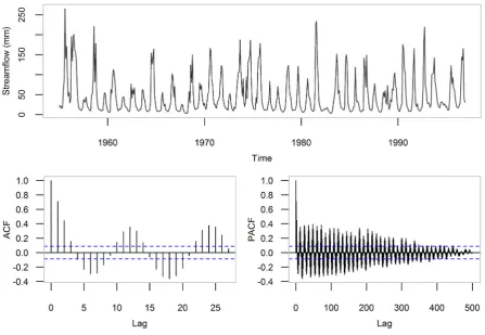
Among these 92 time series, in the present manuscript we focus on Str_77, which is
presented in Figure 1. The length of this specific time series is 42 years (January 1955 to
December 1996) or 504 observations. For its exploration we calculate the sample
Autocorrelation Function (ACF) and the sample Partial Autocorrelation Function (PACF),
which are also presented in Figure 1. The respective H estimate equals 0.90. The use of
this specific time series is not dictated from any significant reason. In fact, we could have
15
Figure 1. The Str_77 time series. Data source: Peel et al. (2000). 2.3 Forecasting methods
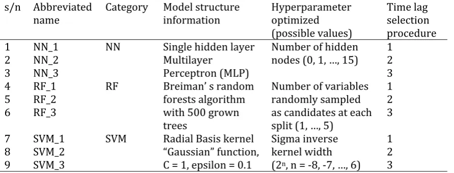
We compare 11 stochastic to 9 ML forecasting methods. The stochastic methods are
classified into five main categories as presented in Table 2. Similarly, the ML methods
are classified into three main categories as presented in Table 3 and Table 4. For the
implementation of the forecasting methods the reader is referred to the Supplementary
16
Table 2. Stochastic forecasting methods. The forecasting methods are available in code form in the Supplementary material.
s/n Abbreviated name Category
1 Naïve Simple
2 RW
3 ARIMA_f ARIMA
4 ARIMA_s 5 auto_ARIMA_f 6 auto_ARIMA_s
7 auto_ARFIMA ARFIMA
8 BATS State space
9 ETS_s
10 SES Exponential smoothing 11 Theta
Table 3. ML forecasting methods. The time lag selection procedures adopted are defined in Table 4. The forecasting methods are available in code form in the Supplementary material.
s/n Abbreviated
name Category Model structureinformation Hyperparameter optimized (possible values)
Time lag selection procedure 1 NN_1 NN Single hidden layer
Multilayer
Perceptron (MLP)
Number of hidden
nodes (0, 1, …, 15) 1
2 NN_2 2
3 NN_3 3
4 RF_1 RF Breiman’ s random forests algorithm with 500 grown trees
Number of variables randomly sampled as candidates at each split (1, …, 5)
1
5 RF_2 2
6 RF_3 3
7 SVM_1 SVM Radial Basis kernel “Gaussian” function, C = 1, epsilon = 0.1
Sigma inverse kernel width (2n, n = -8, -7, …, 6)
1
8 SVM_2 2
9 SVM_3 3
Table 4. Time lag selection procedures adopted for the ML methods. The forecasting methods are available in code form in the Supplementary material.
s/n Time lags
1 The corresponding to an estimated value for the ACF using the acf R algorithm (built in R algorithm), i.e. the time lags 1, …, 20 for a time series of 100 values and the time lags 1, …, 24 for a time series of 300 values
2 The corresponding to a statistical important estimated value for the ACF using the acf R algorithm (built in R algorithm). If there is no statistical important estimated value for the ACF, the corresponding to the largest estimated value
3 According to the nnetar R function (package forecast), i.e. the time lags 1, …, n, where n is the number of AR parameters that are fitted to the time series data using the ar R algorithm (built in R algorithm)
We use two simple forecasting methods in the comparisons. The Naïve forecasting
method, one of the most commonly used benchmarks (Hyndman and Athanasopoulos
2013; Pappenberger et al. 2015), simply sets all forecasts equal to the last value. The RW
17
drawing a line between the first and the last value and extrapolating it into the future
(Hyndman and Athanasopoulos 2013). The stochastic methods also include the ARIMA
and ARFIMA methods. These five methods apply the maximum likelihood method to
estimate the values of the parameters of the AR and MA parts of the models. For the
ARIMA_f and ARIMA_s forecasting methods the numbers of the AR (p) and MA (q)
parameters are set to be the same to those used in the simulated processes, while the
number of differencing (d) is set to be zero. The auto_ARIMA_f and auto_ARIMA_s
methods estimate the values of p, d, q of the ARIMA model using the Akaike Information
Criterion with a correction for finite sample sizes (AICc), as described in Hyndman and
Athanasopoulos (2013). The same applies to the auto_ARFIMA method for the
estimation of the values of p, d, q of the ARFIMA models.
The BATS and ETS_s forecasting methods use the point forecasts from an exponential
smoothing state space model with several key features, i.e. capability of performing
Box-Cox transformation and/or including ARMA errors correction, Trend and Seasonal
components (BATS), also allowing an optimal model selection using the Akaike
Information Criterion (AIC), and an exponential smoothing state space model with
automatic selection of the Error, Trend and Seasonal components (ETS) respectively. We
additionally include the SES (Simple Exponential Smoothing) and Theta forecasting
methods in the comparisons. The latter method was presented by Assimakopoulos and
Nikolopoulos (2000) and had the best performance in the M3-Competition, during
which it was applied to 3 003 historical time series from various categories of data
(Makridakis and Hibon 2000). The reader is referred to Hyndman et al. (2008) and
Hyndman and Athanasopoulos (2013) for the theoretical background of the exponential
18
Regarding the NN, the RF and the SVM forecasting methods, there are some additional
concerns to the selection of the algorithms, originating from the nature of the ML
methods. The choices to be considered for the selection of the time lags used to build the
regression matrix (input data matrix), as well as the choices for the values of the
hyperparameters of the models (e.g. the hidden nodes in a NN model), are many.
Usually, hyperparameters are not directly decided by the ML algorithm during the fitting
process. A fact is that the ML models are by design rather more flexible than needed in
most cases and, thus, hyperparameter optimization is often used to detect and prevent
overfitting as much as possible. In Tables 3 and 4 we summarize the basic information
about the model structures, the hyperparameter optimization and the time lag selection
procedures adopted.
We apply the stochastic methods using mainly the R package forecast (Hyndman and
Khandakar 2008, Hyndman et al. 2017) and the ML methods using the R package rminer
(Cortez 2010, 2016) and the nnetar algorithm from the R package forecast, as also
several built in R algorithms. The R package rminer uses the nnet algorithm of the nnet R
package (Venables and Ripley 2002), the randomForest algorithm of the randomForest
R package (Liaw and Wiener 2002) and the ksvm algorithm of the kernlab R package
(Karatzoglou et al. 2004) for the application of the NN, the RF and the SVM methods
respectively.
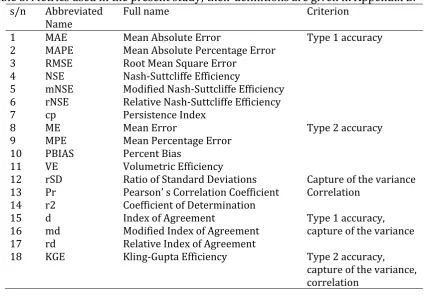
2.4 Metrics
The metrics used for the comparative assessment of the forecasting methods are
classified into five main categories according to the criterion presented in Table 5. They
provide assessment regarding two types of accuracy, the capture of the variance and the
19
the actual, while by Type 2 accuracy we mean the closeness of the mean of the
forecasted values of each time series to the mean of the actual ones. The definitions of
the metrics are listed in Appendix B, while the reader is also referred to Nash and
Sutcliffe (1970), Kitanidis and Bras (1980), Yapo et al. (1996), Krause et al. (2005), Criss
and Winston (2008), Gupta et al. (2009), Zambrano-Bigiarini (2014) for further
information.
Table 5. Metrics used in the present study; their definitions are given in Appendix B.
s/n Abbreviated Name
Full name Criterion
1 MAE Mean Absolute Error Type 1 accuracy 2 MAPE Mean Absolute Percentage Error
3 RMSE Root Mean Square Error 4 NSE Nash-Suttcliffe Efficiency
5 mNSE Modified Nash-Suttcliffe Efficiency 6 rNSE Relative Nash-Suttcliffe Efficiency 7 cp Persistence Index
8 ME Mean Error Type 2 accuracy
9 MPE Mean Percentage Error 10 PBIAS Percent Bias
11 VE Volumetric Efficiency
12 rSD Ratio of Standard Deviations Capture of the variance 13 Pr Pearson’ s Correlation Coefficient Correlation
14 r2 Coefficient of Determination
15 d Index of Agreement Type 1 accuracy, capture of the variance 16 md Modified Index of Agreement
17 rd Relative Index of Agreement
18 KGE Kling-Gupta Efficiency Type 2 accuracy, capture of the variance, correlation
2.5 Methodology outline
For the comparison of the forecasting methods (see Section 2.3) we conduct 12
large-scale computational experiments based on simulations. Within each of the latter we
simulate 2 000 time series according to a model of a stochastic process (see Section 2.1).
We conduct each computational experiment twice; the first time using simulated time
series of 110 values and the second time using simulated time series of 310 values. The
20
Table 6. Simulation experiments of the present study. The simulated processes are presented in Table 1.
s/n Code Simulated
process Length of the time series
1 SE_1a 1 110 values
2 SE_2a 2
3 SE_3a 3
4 SE_4a 4
5 SE_5a 5
6 SE_6a 6
7 SE_7a 7
8 SE_8a 8
9 SE_9a 9
10 SE_10a 10
11 SE_11a 11
12 SE_12a 12
13 SE_1b 1 310 values
14 SE_2b 2
15 SE_3b 3
16 SE_4b 4
17 SE_5b 5
18 SE_6b 6
19 SE_7b 7
20 SE_8b 8
21 SE_9b 9
22 SE_10b 10
23 SE_11b 11
24 SE_12b 12
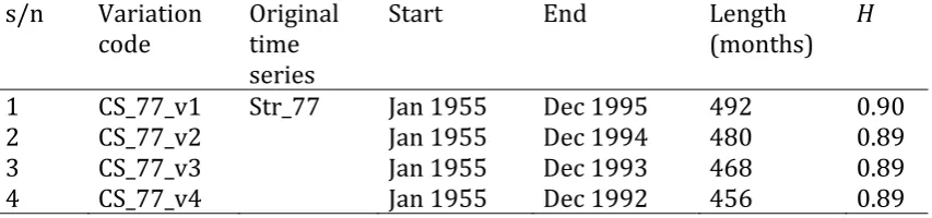
Additionally, we conduct 92 real-world case studies using the time series presented
in Section 2.2. The case studies are respectively named as CS_1, CS_2, …, CS_92 after the
time series Str_1, Str_2, …, Str_92 that they examine. As regards CS_77, we also examine
its 4 variations defined in Table 7. We apply the forecasting methods to the simulated
and the real-world time series according to Table 8.
Table 7. Variations of the CS_77 case study using parts of the Str_77 time series, which is presented in Figure 1. The H parameter is estimated for the deseasonalized time series.
s/n Variation
code Original time series
Start End Length
(months) H
1 CS_77_v1 Str_77 Jan 1955 Dec 1995 492 0.90
2 CS_77_v2 Jan 1955 Dec 1994 480 0.89
3 CS_77_v3 Jan 1955 Dec 1993 468 0.89
21
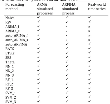
Table 8. Use of the forecasting methods on the time series. Forecasting
method ARMA simulated processes ARFIMA simulated process Real-world time series
Νaive
RW
ARIMA_f × ×
ARIMA_s × ×
auto_ARIMA_f × ×
auto_ARIMA_s × ×
auto_ARFIMA ×
BATS
ETS_s
SES
Theta
NN_1
NN_2
NN_3
RF_1
RF_2
RF_3
SVM_1
SVM_2
SVM_3
For the application of the stochastic methods we divide each time series into two
segments, i.e. the fitting segment and the test segment, which contain n1 and n2 values respectively, as indicated in Figure 2. We fit the stochastic models to the former and
make predictions corresponding to the latter using the recursive multi-step ahead
forecasting method. For the simulation experiments n2 equals 10, while for the real-world case studies 12. For the application of the ML forecasting methods, we
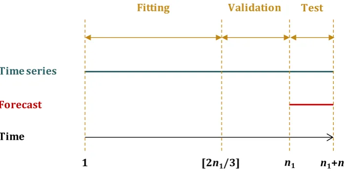
additionally divide the segment of n1 values into two segments, i.e. the fitting segment (first [2n1/3] values of the time series) and the validation segment, as indicated in Figure 3. Regarding the real-world time series, the fitting and validation segments are
used after mean-value deseasonalization, which is performed using a multiplicative
model of time series decomposition. For a brief coverage of the subject of the time series
decomposition methods the reader is referred to Hyndman and Athanasopoulos (2013).
22
also precede the application of most of the stochastic methods. Nevertheless, the ML
methods are non-parametric and, thus, they are not affected by the non-normality.
Figure 2. Division of a time series into two segments for the application of the stochastic methods.
Figure 3. Division of a time series into three segments for the application of the ML methods.
The validation segment serves the hyperparameter optimization procedure, as
explained subsequently. We use the fitting segment to fit several ML models that differ
only as it comes to the values of a specific hyperparameter. We use each of those models
to make predictions corresponding to the validation segment and measure the RMSE of
those predictions. Finally, we decide on the value of the hyperparameter, i.e. the
corresponding to the model with the smallest RMSE on the validation segment Forecast
Timeseries
Time
Fitting
1 n1+n2
Test
n1
Forecast
Timeseries
Time
Fitting Validation
1 [2n1/3] n1+n2
Test
23
(optimum model). We fit a model with the selected hyperparameter value to data of
both the fitting and validation segments and make predictions corresponding to the test
segment. Regarding the real-world case studies, we add the seasonality to the predicted
time series.
To form a qualitative image of the forecasting methods we first apply several diverse
graphical methods on the data sets shaped within each simulation experiment. Here, we
only present forecasting examples on two simulated time series of 110 values in Figures
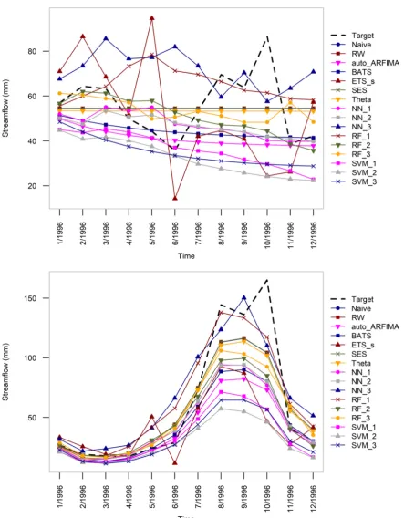
4 and 5, as well as on the Str_77 time series. Figure 6 presents the forecasted time series
within the CS_77 case study with seasonality both included and excluded. The
concomitant to the addition of seasonality improvement of the forecasts is certainly a
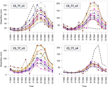
noteworthy fact. Furthermore, Figure 7 presents forecasting examples within the
examined variations of the CS_77 case study highlighting the uniqueness of each
forecasting case. For an extensive graphical exploration of the simulation experiments
24
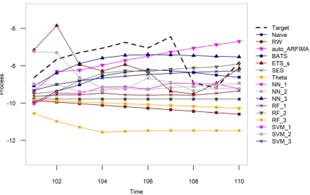
Figure 4. Forecasting examples on a time series resulting from the simulation of an ARMA process within the SE_6a simulation experiment.
25
26
Figure 7. Forecasting examples within the examined variations of the CS_77 case study. Despite its large interest, this specific visualization cannot support a massive and
objective evaluation, which is absolutely essential when pursuing generalized results.
Therefore, we compute the values of the metrics presented in Section 2.4 for each
forecasting test. The computation takes place on the test segment, which functions as a
reference for the comparative assessment of the forecasting methods’ performance.
Finally, we calculate several descriptive statistics, namely the minimum (min),
maximum (max), mean, median, standard deviation (sd), interquartile range (iqr),
kurtosis and skewness, of the metric values distributions for all the forecasting tests
related to each forecasting method within each forecasting experiment. We use those
values for the comparative assessment of the forecasting methods, mainly the medians
27
the comparison of the values of the each metric computed within the case study, while
the smallest the iqr the better the forecasts.
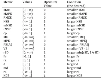
Table 9. Use of the metrics for the comparative assessment of the forecasting methods. The metrics are defined in Appendix B.
Metric Values Optimum
Value Condition (the desired) MAE [0, +∞) 0 smaller MAE MAPE [0, +∞) 0 smaller MAPE RMSE [0, +∞) 0 smaller RMSE NSE (-∞, 1] 1 larger NSE mNSE (-∞, 1] 1 larger mNSE rNSE (-∞, 1] 1 larger rNSE
cp (-∞, 1] 1 larger cp
ME (-∞,+∞) 0 smaller |ME| MPE (-∞,+∞) 0 smaller |MPE| PBIAS (-∞,+∞) 0 smaller |PBIAS| VE (-∞,+∞) 1 smaller |VE - 1|
rSD [0, +∞) 1 larger min{rSD, 1/rSD}
Pr [-1, 1] 1 larger Pr
r2 [0, 1] 1 larger r2
d [0, 1] 1 larger d
md [0, 1] 1 larger md
rd (-∞, 1] 1 larger rd
KGE (-∞, 1] 1 larger KGE
Although our computational experiments are designed to produce new knowledge in
the field of time series forecasting, there are several outcomes rather well known at the
forefront of our methodological framework (benchmarking). In more detail, the ARIMA_f
and also the auto_ARIMA_f forecasting methods are expected to have the best
performance regarding the Type 1 accuracy, mainly in terms of RMSE, on the time series
resulting from the simulation of ARMA processes because of their theoretical
background (for details see Wei 2006, pp. 88-93). Likewise, this applies to the
performance of ARIMA_s and auto_ARIMA_s regarding the capture of the variance
exhibited by the time series within the same simulation experiments. Furthermore, the
ARIMA_f and ARIMA_s forecasting methods share an additional advantage, since they
use by design the p, d, q numbers used in the simulation process. Similarly to the
28
best in terms of RMSE on the time series resulting from the simulation of ARFIMA
processes. The five forecasting methods mentioned in the present paragraph, together
with the two simple methods, play a key role within our methodological approach.
The results are presented in the context of an exploratory visualization and are
available in both quantitative and qualitative forms. All numerical results are provided
in table form, while the graphs implemented include histograms, barplots, side-by-side
boxplots and heatmaps. This specific context facilitates the comparisons in an efficient
way, as it ensures the multifaceted representation of the information provided.
Furthermore, the heatmap visualization within and across the various simulation
experiments eases the detection of systematic patterns that are closely related to
theoretical elements. Therefore, we emphasize on the qualitative form of the results. For
the simulation experiments, we mainly focus on two general categories of heatmaps, i.e.
the “Type 1 heatmaps” and “Type 2 heatmaps”, which use the median values of the
metrics. The former type integrates the information provided by all metrics for the
average-case performance of the forecasting methods within a specific simulation
experiment, while the latter imprints the average-case performance of the forecasting
methods across the various simulation experiments according to a specific metric.
3. Results
3.1 Simulation experiments
Section 3.1 aims at providing a synopsis of the results of the simulation experiments.
The latter constitute the basis for the comparison of the forecasting methods on a
theoretical level. To support our key findings, which are derived through a
comprehensive examination of the results, here we present a small, though
29
Supplementary material for a thorough overview of the simulation experiments. We
especially encourage the reading of Section 3.1 alongside with the report entitled
“Selected figures for the qualitative comparison of the forecasting methods’’ of the
Supplementary material.
We choose to start our brief exploration into the simulation experiments by
presenting the descriptive statistics calculated for the distributions of the NSE metric
values within the SE_1a simulation experiment (see Table 10). This choice is prompted
by the fact that the NSE is a metric particularly important for the field of hydrology. In
fact, if we had to base our comparisons to one metric, this would probably be this
specific one. While examining the numerical results under discussion, we most
importantly note that the medians are all negative, which means that at least the 50% of
the forecasts given by all the forecasting methods are less close to their corresponding
values than the mean of the latter. Secondly, we proceed to ranking the various
forecasting methods according to the median (or the mean) values and the condition
stated on Table 9. We note that ARIMA_f produces the best forecasts in terms of NSE, as
assumed in Section 2.5 for several metrics providing assessment regarding the Type 1
accuracy. We also observe that the simple methods have a rather moderate than bad
performance in terms of NSE, since they are better than four forecasting methods,
namely ARIMA_s, auto_ARIMA_s, ETS_s and NN_1. Additionally, we note that the sd or iqr
values also vary significantly from one forecasting method to the other, with the latter
mentioned forecasting methods being worse than the rest also regarding these
descriptive statistics. Up to this point, we surely have started to wonder how different
the forecasting methods’ ranking would be, if we had examined the results provided by
some other metric for the same simulation experiment. Furthermore, we wonder in
30
Table 10. Descriptive statistics calculated for the distributions of the NSE metric values for all forecasting tests within the SE_1a simulation experiment. The simulation experiments are named according to Table 6.
min max mean median sd iqr kurtosis skewness
Naïve -38.176 0.000 -2.109 -0.896 3.426 2.306 19.912 -3.706 RW -41.012 0.112 -2.337 -1.004 3.787 2.571 20.082 -3.740 ARIMA_f -24.000 0.651 -0.901 -0.346 1.746 1.156 42.554 -5.159 ARIMA_s -52.813 0.823 -3.112 -1.899 4.192 3.212 29.047 -4.123 auto_ARIMA_f -30.074 0.639 -1.185 -0.421 2.342 1.273 38.271 -5.002 auto_ARIMA_s -186.344 0.734 -4.343 -2.277 8.392 3.977 156.028 -9.706 BATS -32.517 0.598 -1.303 -0.476 2.404 1.388 34.249 -4.643 ETS_s -137.892 0.804 -7.678 -3.642 12.071 7.594 28.102 -4.332 SES -37.180 0.000 -1.921 -0.791 3.107 2.131 22.453 -3.785 Theta -37.478 0.055 -1.944 -0.809 3.143 2.160 22.116 -3.773 NN_1 -85.677 0.697 -3.132 -1.660 5.417 3.268 67.804 -6.464 NN_2 -822.800 0.655 -1.919 -0.612 18.602 1.521 1893.157 -42.990 NN_3 -578.538 0.773 -1.422 -0.431 13.091 1.271 1885.438 -42.856 RF_1 -39.846 0.790 -1.344 -0.532 2.728 1.419 64.811 -6.464 RF_2 -39.379 0.769 -1.401 -0.594 2.699 1.483 51.352 -5.742 RF_3 -38.670 0.713 -1.602 -0.772 2.518 1.815 37.973 -4.495 SVM_1 -39.495 0.810 -1.396 -0.614 2.763 1.470 65.887 -6.537 SVM_2 -37.764 0.715 -1.327 -0.571 2.370 1.480 44.327 -4.967 SVM_3 -31.314 0.765 -1.094 -0.409 1.970 1.248 40.159 -4.648
Before answering the above worded questions, we consider important to report some
preliminary observations extracted from Table 10, but also verified for the rest of the
numerical results. Regarding the kurtosis and skewness values, these indicate that the
measured NSE metric values are not normally distributed. This specific observation
introduces several issues in handling the metric values for the purposes of the present
study, which we overcome by basing our comparisons mainly on the medians and the
iqr values, as well as by removing the (far) outliers from the figures. Noteworthy is also
the fact that the above worded observation does not apply to all of the metrics equally
and, thus, we could claim that there are metrics more manageable than others. In fact,
although we focus on the comparison of the forecasting methods, the interested reader
could discover worth considered information about the metrics in the Supplementary
31
because of their far outliers. The latter is a clear sign of instability, while the ARIMA_s,
auto_ARIMA_s, ETS_s and NN_1 forecasting methods seem to share a different form of
instability. Finally, we note the great similarity that the distributions measured for the
SES and Theta forecasting methods exhibit, which applies to all the distributions
measured for these specific forecasting methods within the present study, confirming
the findings of previous studies, e.g. Hyndman and Billah (2003). This similarity is,
however, of secondary importance here.
Next, we choose to navigate within the SE_1a simulation experiment using a
simplified form of the distributions of the metric values (see Figures 8-10). This specific
navigation is indicative of the navigation within any other simulation experiment, and,
thus, of great importance in yielding valuable insights into the nature of hydrological
time series forecasting, as well as in comparing the forecasting methods or the
information provided by each metric regarding the latter.
Some important observations applying to all the simulation experiments are reported
subsequently. First, we observe that even the relative metrics, i.e. the corresponding to
the same criterion (see Table 5), provide measurements which lead us to different
aspects of the same information to an extent bigger or smaller depending on the pair of
metrics compared. Second, we note that some of these 18 different aspects are also
conflicting to each other and, hence, we realize that we cannot decide on a general
ranking of the forecasting methods using the results of a specific simulation experiment,
unless we introduce extra constraints. In more detail, we would have to select the
criterion and, furthermore, the metric of our interest, for this specific ranking to be
possible. Third, we perceive that the collective examination of the quantitative form of
the results is quite challenging and, thus, the imposition of a simplification procedure is
32
33
34
Figure 10. Side-by-side boxplots for the comparative assessment of the forecasting methods regarding their performance within the SE_1a simulation experiment (part 3). Concerning the boxplots of the metrics rd and KGE, the far outliers have been removed.
To this end, in Figure 11 we present the Type 1 heatmaps for the comparison of the
35
Additionally, in Figures 12-17, we present the Type 2 heatmaps according to the RMSE,
PBIAS, rSD, Pr, d, KGE metrics respectively. In the heatmaps the scaling is performed in
the row direction and the darker the colour the better the forecasts. We have also
applied clustering analysis on the forecasting methods based on their performance.
Having moved step-by-step from the level of a specific metric to the collective
examination of the information provided by all the 18 metrics within a specific
simulation experiment and subsequently to the collective examination of the entire
information using the Type 1 and Type 2 heatmaps, we devote the following paragraphs
in summarizing the outcome of the simulation experiments. Figures 11-17 together with
Figures 8-10 can facilitate the reading of this synopsis in a rather satisfactory manner.
Regarding the decoding of the information provided by the conducted heatmaps, an
example is available in Section 3.2.
Admittedly, the most significant outcome of the present study is that none of the
forecasting methods is found to be better or worse than the rest regarding all the
metrics employed in the evaluation process simultaneously. Alternatively worded, none
of the forecasting methods is uniformly best or worst. This observation, first obtained
for the SE_1a simulation experiment through the collective examination of Figures 8-10,
is easily confirmed for the rest of the simulation experiments using the Type 1
heatmaps, while it reveals that the forecasting quality is subject to limitations. However,
there are forecasting methods regularly better or worse than others according to
specific metrics, as well as forecasting methods sharing a quite similar performance (e.g.
Naïve and RW). The latter easily becomes evident through the examination of the Type 2
heatmaps. For instance, the ARIMA_s, auto_ARIMA_s and ETS_s forecasting methods
exhibit far the best average-case performance in terms of rSD for all the simulation
36
selection of the optimal forecasting method/methods for various engineering
applications and also allows the wording of several advantages/disadvantages to some
extent, as well as a preliminary clustering of the forecasting methods. Of course, this fact
does not apply to all the forecasting methods neither to all the metrics. For example, we
observe that the Theta forecasting method can exhibit good, moderate or bad
average-case performance in terms of KGE depending on the simulation experiment (see Figure
17), while none of the forecasting methods is found to be regularly better or worse in
respect to PBIAS (see Figure 13).
In summary, each forecasting method has some specific theoretical properties and,
due to the latter, it performs better or worse than others with respect to specific metrics
and/or within specific simulation experiments. We note that the former observations
apply equally to the stochastic and the ML forecasting methods. Therefore, forecasting
methods originating from both the main categories are found amongst the first, as well
as the last positions in each resulting ranking. The latter is possible for a specific metric
within a specific simulation experiment. Furthermore, it is noteworthy that Naïve and
RW are also competent. These simple methods exhibit rather the best average-case
performance in terms of d (see Figure 16) and md. Naïve and RW also perform better or
equally well to other forecasting methods regarding several metrics within specific
forecasting experiments. We also note that the values of the metrics can vary
significantly across the different time series, while in general this variation depends on
the metric and the forecasting method and can be extracted from the quantitative form
of the results (see for example Figures 8-10). The observations outlined above hold a
complete explanation of the results derived by Papacharalampous et al. (2017).
Another important outcome resulting from the examination of the Type 1 heatmaps is
37
and the clustering of the forecasting methods to a smaller extent than the simulated
process. In more detail, the length of the time series affects the performance of the NN_1
forecasting method largely, while the performance of the rest forecasting methods is less
or even slightly affected depending on the forecasting method as also on the simulated
process. Moreover, we observe that forecasting methods resulting from the
implementation of the same algorithm can exhibit a far distant or always close
performance depending on the algorithm. For instance, the ARIMA forecasting methods
can differ with each other to a great extent, a fact also applying to NN, but not to the RF
and SVM forecasting methods. Additionally, we note that some of the Type 2 heatmaps
are rather smoother than other heatmaps of the same category (see for example Figures
12-17), as the variability across the different simulation experiments can be larger or
38
39
40
41
42
43
44
45
3.2 The CS_77 case study (and variations)
In full correspondence to the simulation experiments, the results of the CS_77 case study
are presented in both quantitative and qualitative forms in Figures 18-20 and Figure 21
respectively. Some information extracted from the numerical results regards the
improvement of the forecasting outcome, when the forecasts are produced using the
deseasonalized time series and subsequently recovering the seasonality, a fact apparent
even in Figure 6. The satisfactory values measured for the NSE, mNSE, rNSE, Pr, r2, d, md
and rd metrics, in comparison to their corresponding distributions resulted from the
simulation experiments (see for example Figures 8-10) are indicative of this specific
improvement. For the qualitative comparison of the forecasting methods’ performance
within the case study under discussion, we can either examine collectively the presented
barplots, or alternatively, mine the information provided by the heatmap, for example as
presented subsequently. While trying to decode Figure 21, we first note that the
performance of SVM_1, SVM_2 and SVM_3 is similar and largely different from the
performance of the rest forecasting methods. Such similarities and differences are
clearly the reason for the clustering accompanying the qualitative representation of the
numerical results. This clustering is illustrated with a proper column rearrangement as
also a cluster dendrogram and has proven its usefulness in the decoding processes.
Furthermore, we note that the forecasts resulting from the SVM algorithm are
amongst the worst regarding the information provided by several metrics, but rather
satisfying in respect to other metrics and the best in respect to VE. The same applies to
the forecast resulting from the ETS_s forecasting method, although the quite good
performance in its case is measured in terms of ME and VE. This specific forecasting
46
exhibit a rather moderate overall performance. Amongst the latter forecasting methods,
RF_2 produces the best forecasts within our case study. Another formed cluster is
composed of the NN_3 and RF_1 forecasting methods. Those two ML methods share, in
fact, a quite similar performance within this real-world case study, although the forecast
resulting from the implementation of RF_1 is clearly better, as well as the best amongst
all the forecasting methods in terms of rSD and KGE. Finally, the cluster exhibiting the
best overall performance includes Naïve, RW, SES and Theta, as also RF_3. The forecasts
resulting from the former four forecasting methods are rather equivalent and better
47
48
49
50
Figure 21. Heatmap for the comparative assessment of the forecasting methods within the CS_77 case study according to the values of the metrics and the conditions listed on Table 9.
The CS_77 case study validates the core findings of the present study, while focusing
on a particularly interesting individual case that would have stayed hidden otherwise.
As in the simulation experiments, here again none of the forecasts is found to be better
or worse than the rest in respect to all the metrics simultaneously and, consequently, we
cannot decide on a uniformly best or worst forecasting method, not even for the single
case under discussion. Additionally, it seems that the forecasts resulting from both the
main categories of forecasting methods are rather equally competent and subject to
limitations. Furthermore, any ranking of the forecasting methods would require the
prior selection of a metric of interest, while the clustering presented in Figure 21 would
be totally meaningless beyond this specific case study. Moreover, away from the
expected results, Naïve and RW are despite their indisputable simplicity amongst the
51
Finally, in Figure 22 we present the results of the examined variations of CS_77.
Clearly, the relative performance of the forecasting methods is completely different
across the five related experiments, a fact rather indicating that the best forecasting
method might depend largely on the forecasting case itself and, thus, might vary, even
when trying to predict in different time moments a specific process at a specific location,
given a slightly different amount of observations at each experiment. This is another
52
Figure 22. Heatmaps for the comparative assessment of the forecasting methods within the variations of the CS_77 case study according to the values of the metrics and the conditions listed on Table 9.
3.3 A collection of 92 real-world case studies
Being familiar with the results presented in Sections 3.1 and 3.2, the reader will not be
53
However, since such collections are rare in the literature, we encourage the reading of
the report entitled “Qualitative comparison of the forecasting methods in 92 real-world
case studies” of the Supplementary material. Although we specifically focus on CS_77
(and its variations) herein, all of the real-world case studies conducted could be used to
confirm the findings of Section 3.1 in an equally satisfactory manner, while the entire
collection highlights the individuality of each case. The same applies to the multiple-case
study conducted by Papacharalampous et al. (2017).
4. Discussion
4.1 Contribution in hydrology and beyond
The present study aims to contribute in hydrology (and beyond) in two direct ways and
indirectly. Our generalized findings, derived in Section 3.1 and validated in Sections 3.2
and 3.3, can provide new insights into the nature of hydrological time series forecasting.
This first direct contribution can be summarized with the following
context-independent research questions and answers, which might be of scientific and/or
practical interest:
Do the ML methods exhibit different forecasting performance from the stochastic? No,
stochastic and ML methods can share a quite similar forecasting performance.
Is it possible for two forecasting methods resulting from the implementation of the same
algorithm to exhibit a far distant performance? Yes, it is possible for stochastic and ML
algorithms.
To which extent might the performance of a specific forecasting method differ across
the various cases of time series? To an extent smaller or larger depending on various
factors, such as the forecasting method, the criterion of interest and the process under