A Multi-Resolution Approach for Audio Classification

A

multi-resolution

approach

for

audio

classification

Sergey

Voronin

and

Alexander

Grushin

1

_Intelligent

_Automation,

_Inc.,

_Rockville,

_MD

Abstract

Wedescribeamulti-resolutionapproachforaudioclassificationandillustrateitsapplicationtotheopendata set for environmental sound classification. The proposed approach utilizes a multi-resolution basedensemble consistingof targetedfeature extraction of approximation(coarsescale) anddetail(fine scale)portions ofthe signal under the actionof multiple transforms. This is pairedwith an automaticmachine learning enginefor algorithmand parameterselectionandtheLSTM algorithm, capableof mapping severalsequencesof features to a predicted class membership probability distribution. Initial results show an improvement in multi-class classificationaccuracy.

1

Introduction

Inmanyapplicationssuchasemotiondetection,itisnecessarytoclassifyanaudiosignalintooneofN available categories. Inthe case of the open dataset for environmental sound classification [11] which we make use of, 10categories offiles are presentwith 40 filesin each category: 001 - Dog bark, 002 -Rain , 003 - Sea waves , 004 -Baby cry , 005 - Clocktick , 006 - Personsneeze , 007 -Helicopter , 008 - Chainsaw, 009 - Rooster, 010 -Fire crackling. Theclassic problemof classification consists of splitting upthewhole set (of400 audio files)intoa training andtesting set, trainingaclassifier, andclassifyingthefiles inthe testingset, whosetrue labelshavebeenremoved. Thisisaccomplishedbycollectingasetoffeaturesfromthetrainingset,normalizing (so all feature valuesfall in the same range), and passing on the feature table along with the class numbers (labels)toasingleclassifierfortraining. Theclassifieristrainedbasedonaselectedalgorithmanditsassociate hyper-parameters as chosen bythe user. An alternate approach uses anensemble of several classifiers (based ondifferentmachinelearning algorithmsor similaralgorithms withdifferent hyper-parametersets). Labelson thetestingset are then assignedeither basedon a singleclassifier or one.g.,the mode predictionas givenby multipletrainedclassifiers.

In this article, we present a multi-classifier ensemble approach where different classifiers are trainedon a multi-resolutionanalysis(MRA)representationoftheaudiosignals[6],obtainedbyinvertingjustthedetailand justthe approximationcoefficientsobtained from a set ofwavelet transforms for eachaudio signal. MRA for classificationhasbeendescribedpreviouslyviaprojections[9],orapplicationofwavelettransformstothefeature sets[12]. Asimilarapproachisdescribedin[2]. Inthisarticle,weexplicitlypresentthedetailandapproximation constructions(reconstructionsatdifferentscales)and utilizetheLSTMalgorithmontheresultingfeature sets, taking as input all representation sequencesfor training. We combinethis with anensemble of classifiers for eachscalerepresentation,obtainedfrom anauto-mlimplementation. Wedescribesomeapproachesto combine

the classifier results for each test sample, based on the probability membership information provided by each classifier.

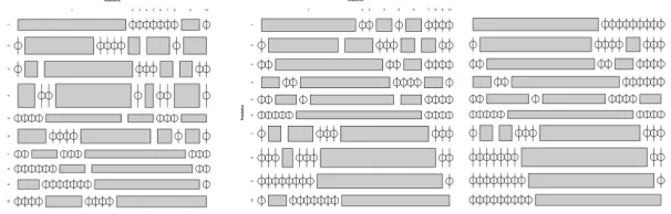
In Figure 1 below, a model is decomposed into coarse and fine parts. With the same logic, we can break the audio signal into different scales and compare different parts individually to corresponding parts of different audio waveforms. If we takepbasis W1, . . . , Wp, then corresponding to original audio signals, we can obtain the transformation [wa, wd] =Wis, where wd are the detail wavelet coefficients and wa are the approximation coefficients. Depending on the number of levels of the transform we perform, we can further sub-dividewd into several different scales. Following this logic and lumping all the detail coefficients together, we can form the approximation and detail portions of the audio signalsvia the computations

asi =W

−1

i [wa; 0], dsi =W

−1

i [0;wd]. (1.1)

A classification may be easier to do over finer scales than the coarser ones, or vice versa. We train a separate classifier for each feature set corresponding to the original signalsand the pairsasi, dsi fori= 1, . . . , p. These

M = p+ 1 audio signals yield M separate feature sets over the test samples (features can be extracted from each representation as though it is a standalone audio signal). The resulting feature sets can be used to train M classifiers, used in an ensemble to yield a prediction (based for example, on the per-class probabilities given by each classifier, as we describe).

Figure 1: Example of model decomposition into different representations, based on a two level wavelet transform.

First row: original model, numbers of approximation and detail coefficients. Bottom row: reconstructions due

only to inverse transform of approximation and individual sets of detail coefficients.

2

Data preparation and audio feature extraction

We now describe the data preparation and feature extraction steps. In particular, we summarize the features we extract for each of the p+ 1 representations (data sets) we obtain for each audio signal s. The first data set consists of theR audio waveforms comprising the training samples. (In the results we present below, we subdivided 320/80 for training and testing portions). For the next sets we obtain either the approximation or detail portions, according to relations (1.1). This can be accomplished in Python using the following code sequence with the Python-Wavelets package, wherey is a vector holding the audio waveform data:

d b o b j = p y w t . W a v e l e t ( t r a n s f o r m _ n a m e ) ;

cA4 , cD4 , cD3 , cD2 , cD1 = p y w t . w a v e d e c ( y , dbobj , m o d e = ’ c o n s t a n t ’ , l e v e l =4)

c o e f f s [ 1 ] = np . z e r o s ( len ( c o e f f s [ 1 ] ) ) c o e f f s [ 2 ] = np . z e r o s ( len ( c o e f f s [ 2 ] ) ) c o e f f s [ 3 ] = np . z e r o s ( len ( c o e f f s [ 3 ] ) ) c o e f f s [ 4 ] = np . z e r o s ( len ( c o e f f s [ 4 ] ) ) e l s e :

c o e f f s [ 0 ] = np . z e r o s ( len ( c o e f f s [ 0 ] ) )

y = p y w t . w a v e r e c ( coeffs , t r a n s f o r m _ n a m e ) ;

The approx portion flag controls whether the approximation or detail portion of the signal is computed. Features can then be extracted from the reconstructedy vector. The features we use are standard for audio analysis and classification work and slightly different features may yield better or worse results. We seek to extract features from an audio waveform as plotted in Figure 2. In order to perform feature extraction, we can make use of

-1 -0.8 -0.6 -0.4 -0.2 0 0.2 0.4 0.6 0.8 1

0 5000 10000 15000 20000 25000 30000 35000 'wav_out'

Figure 2: Sample waveform wav file

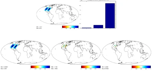
various openly available software. In Python, the librosa package (https://librosa.github.io/) provides good audio processing functionality and can return the value of many relevant parameters. In addition, the waveform can be analyzed as a time series. Packages such as tsfresh (https://pypi.python.org/pypi/tsfresh) allow for efficient feature extraction. Finally, for pitch and beat detection, we make use of the https://aubio.org/ library. In this report, we analyze the application of the discussed MRA scheme to, applied to the excellent ESC-10 data set [11] (https://github.com/karoldvl/ESC-10,https://github.com/karoldvl/ESC-50). In Figure 3, we plot some examples of features used in [10]. In particular, we plot the distribution of the so called MFCC (mel-frequency

Figure 3: Feature extraction for the ESC-10 data set [11].

spectral, time series), provide a good identification footprint. Below, we list the features we have extracted and the reasoning behind them.

• MFCC coefficients and ZCR values. Time-frequency representation features heavily used in audio classifi-cation work.

• Spectral features (spectral centroid, rolloff, tonal centroid). Various measures associated with the spectro-gram (visual representation of frequency spectrum of the waveform as a function of time).

• RMSE of signal frames and tempo. Associated with aspects such as variations in loudness of ones voice.

• Beat information (tempo, onset times). Associated with e.g. speed and pauses in speech.

• Pitch information, the perceived height of musical notes. Particularly, streak lengths of high pitch are measured.

• Wavelet representation statistics in smooth and sharp basis, such as the norms of approximation and detail coefficients.

• Several statistics extracted from the time series: mean second derivative, longest streak above the mean, kurtosis, mean auto-correlation, time reversal asymmetry statistic.

The above statistics represent a good mix of features related to an audio signal, its spectrum, and to its representation as a time series. The inclusion of a few more statistics is plausible, for example some features based on dynamic time warping may aid in classification. The above parameters can take a range of different values. Simple rescaling is done according to the formula _max(xx₎−₋x¯_min(x), with ¯xthe mean ofxfor each column of the resulting feature matrix. This formula is applied for each column of the resulting feature matrix (the set of the same parameter values over all audio frames). This way, all values of parameters occur on the interval (0,1) so that no feature is weighed significantly more than another during classification (unless of course, one may want some features to weigh more than others, in which case custom scaling may be plausible). It should be noted that the rescaling factors are often saved, so that new audio files which need to be classified can undergo feature extraction and then rescaling with the same factors.

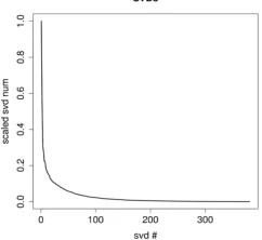
With the MRA approach, redudancy is possible. That is, if two wavelet basis used are similar to one another (e.g. both correspond to smoothing filters of similar type) the feature sets for each audio signal will be similar and approximate linear dependence will result. To check, it is enough to append all the feature matrices into a single matrix and observe the rate of decay of the corresponding singular values. While the decay is expected to be nonlinear, the dropoff should be modest enough such that several sets of features are of significance of significance. Combining our 9 feature sets side by side, the singular value drop off is shown in Figure 4. We

Figure 4: Singular values of appended mega matrix for all feature sets.

to choose more distinct transformation bases to reduce linear dependence and further improve the classification results.

3

Per class analysis with KNN

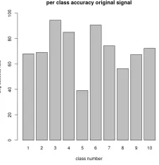
In Figure 5 below, we plot the average accuracy of the simple k nearest neighbors algorithm (withk= 12) over 150 randomly shuffled instances of the data set with the training portion set to 320 out of 400. The overall avg accuracy and per class results are plotted in Figure 5 below. We obtain about 71.6% average accuracy over 150 trials. In the same figure, we have also plotted the average accuracy per class. We can see that certain classes are harder to classify than others. For example, the avg success rate for class 5 - ‘clock tick’, was low. Next, we analyze the per class avg accuracy for the approximation and detail representations corresponding to 4 wavelet bases: Haar, DB4, Bior 3.9, Rev Bior 3.9. These 4 bases are frequently employed in signal processing and are designed to capture different portions of the signal (e.g. Haar for sharper features and DB4 for coarser level features). We take transforms with respect to the four bases and invert back only keeping either the approximation coefficients or the detail coefficients to be nonzero. This then results in 8 additional representations of each audio signal (complementing the original) from which we can extract features. We take exactly the same subset of training and testing portions for each set to produce the results in Figure 6, where we plot the per-class accuracy as given by classifiers derived from each of the 8 wavelet based signal representations.

Figure 5: Average accuracy of KNN method (k=12) by class as recorded for random 320/80 train/test splits over

multiple runs.

Figure 6 shows the by class accuracy obtained on the full and inverse transformed data, as well as the average F-scores for each of the 9 (1 full and 8 transformed) feature sets from cross validation. The overall classification accuracy obtained via the transformed data in Figure 6 is worse than on the untransformed data in Figure 5. On the other hand, certain classes are better resolved by the transformed data. As an example, the inverse transformed data of the detail coefficients of the rbio3.9 wavelet (reverse-biorthogonal family), lends itself slightly better to class 5, which still remains ill-resolved by most representations. However, the results suggest that an ensemble method consisting of classification results obtained for the original and transformed representations would yield better performance over all classes.

4

Auto-ml and LSTM approach with MRA ensemble method

Figure 6: Left: Average accuracy of KNN method (k=12) by class using full and inverse transformed approximation

and detail data. Right: average F-scores for 5 fold CV with the different feature sets.

(https://www.cs.ubc.ca/labs/beta/Projects/autoWeka/) in Java. The source code to replicate the results re-ported here can be found at: https://github.com/sergeyvoronin/multi resolution classification. To perform clas-sification, we may either choose a single method such as e.g. the Multi-Layer Perceptron and its associated parameter values (number of layers, learning rate, etc) to use for each training / testing set consisting of 400 audio signalssand their associated approximate and detail representationsai, di; or, we can utilize an automatic machine learning approach, which by use of Cross validation over each training set we supply, finds a particular algorithm and a set of hyper-parameters which optimize a defined performance metric [13]. The auto-Weka package consistently gives solid performance, provided enough time and memory resources are allocated for its use. This can be controlled in Java via a set of parameters. For example, the following code snippet will run the auto-ml code for 10 mins on the supplied training set and build a suitable classifier:

A u t o W E K A C l a s s i f i e r awc = new A u t o W E K A C l a s s i f i e r () ; awc . s e t T i m e L i m i t ( 1 0 ) ;

awc . b u i l d C l a s s i f i e r ( t r a i n ) ;

The performance of the ensemble method depends on how we choose to combine the results of different classifiers, trained (in our case) on one of the nine training sets, corresponding to the same file ordering. A simple approach is to take the mode of the nine predictions for each element of the test set. A different approach is to utilize the per-class probabilities outputted by the Weka based auto-Weka classifier. In addition to outputting the predicted class, the per class probabilities are obtained from the calls:

d o u b l e l a b e l = awc . c l a s s i f y I n s t a n c e ( t e s t . i n s t a n c e ( i ) ) ;

We can utilize this information to get a mean probability for each class, out of the 9 available classifiers. Then the output label would simply be the class name corresponding to the highest mean probability. Of course, a more advanced Bayesian statistical approach is also possible and described below. Finally, we can also take some hybrid approach, where we only combine predictions that match a given lower bound probability for the predicted class (i.e. 60%). To supplement the above approach, we can apply the long short-term memory (LSTM) algorithm to the MRA representations [3]. LSTM is a recurrent neural network that can learn to classify a sequence of inputs, rather than individual inputs (see Figure 7). Although it accepts the sequence one input at a time, it is able to remember relevant information from the inputs, in order to make a classification decision. Information is stored in specialized memory neurons, and their activity is modulated by gate neurons. The input gates determine the extent to which the current input should be stored in memory; the forget gates determine how much memory is retained between time steps (allowing unnecessary memory contents to be cleared), and finally, the output gate modulates the effect of memory upon the current output. In turn, the operation of the gates is affected by the memory contents (dashed arrows from the memory layer to the gate layers). While it is common for the sequence to be temporal in nature (e.g., each input is a set of measurements taken at some time), we can similarly apply LSTM to MRA data, by treating each representation as an input, and thus providing a sequence of resolutions/scales. LSTM MRA based classification can easily be implemented in Python with the

Figure 7: The standard LSTM architecture [8].

Keras library. The construction proceeds by concatenating sequences of features (from the untransformed signal and 8 transformed sets, corresponding to the approximation and detail portions under the transformations we consider) for each audio signal (separately for the training and testing sets):

seq = [ np . a r r a y ( u n t _ r o w s [ i ]) , np . a r r a y ( w a v 1 a p _ r o w s [ i ]) , np . a r r a y ( w a v 1 d l _ r o w s [ i ]) , np . a r r a y ( w a v 2 a p _ r o w s [ i ]) , np . a r r a y ( w a v 2 d l _ r o w s [ i ]) , np . a r r a y ( w a v 3 a p _ r o w s [ i ]) , np . a r r a y ( w a v 3 d l _ r o w s [ i ]) , np . a r r a y ( w a v 4 a p _ r o w s [ i ]) , np . a r r a y ( w a v 4 d l _ r o w s [ i ]) ]; X . a p p e n d ( seq ) ;

This results in two three dimensional tensors (for testing and training). For example, with our split our tensors have the dimensions Xtr: (320,9,53) and Xtest: (80,9,53) where the dimensions reflect the number of samples (audio files) in each set, number of sequences, and number of features in each sequence. The class labels (for training and testing sets) must be transformed to categorical matrix form (a sparse matrix with a singe one in each row, corresponding to the label). This can be accomplished as follows:

y t r _ c a t = t o _ c a t e g o r i c a l ( ytr -1 , n u m _ c l a s s e s = 1 0 ) y t e s t _ c a t = t o _ c a t e g o r i c a l ( ytest -1 , n u m _ c l a s s e s = 1 0 )

where the labels assigned are in the range 0 to 9 for the 10 classes. An LSTM model is then built with a variable number of hidden layers. Different settings can be attempted. As an example, we may use the softmax activation function and categorical cross entropy loss (objective score) which is attempted to be minimized during training:

m o d e l = S e q u e n t i a l ()

m o d e l . add ( L S T M (80 , r e t u r n _ s e q u e n c e s = True , i n p u t _ s h a p e =(9 , 53) ) ) m o d e l . add ( L S T M (80 , r e t u r n _ s e q u e n c e s = T r u e ) )

m o d e l . add ( L S T M ( 8 0 ) )

l o s s = ’ c a t e g o r i c a l _ c r o s s e n t r o p y ’ , m e t r i c s =[ ’ a c c u r a c y ’ ])

Then we can fit the model and get predictions by taking the argmax of each output sequence for each member of the testing set:

m o d e l . fit ( Xtr , ytr_cat , e p o c h s =200 , s h u f f l e = F a l s e ) y h a t = m o d e l . p r e d i c t ( Xtest , v e r b o s e =0)

for i in r a n g e (0 , len ( y h a t ) ) :

m a x _ i n d = np . a r g m a x ( y h a t [ i ]) + 1 p r i n t f ( " p r e d i c t i o n = % d \ n " , m a x _ i n d ) p r i n t f ( " a c t u a l = % d \ n " , y t e s t [ i ])

Several methods for combining classifiers to obtain more accurate per class probabilities for each test sample can be utilized [4]. Suppose that we haveM = 9 MRA feature sets as described from the original audio signal and the prepresentations at different scales: S1, . . . , SM. For a given test sample, we can use a classifier on set Sk, with k ∈[1, M] to query its class membership probability for each class i. Let us call this probability P(Ci|Sk), with i∈[1,N¯], with ¯N the number of classes (10 for the ESC-10 set). We are interested to combine these probabilities for eachk, to get a probability for classimembership of the test samples based on all theM feature sets Perhaps the simplest is to average the probability per class of each classifier, yieldingPM

k=1

P(Ci|Sk)

M for eachi. The guessed membership class for a particular test sample is then determined by the highest average probability among alliclasses (argmax). A slight twist on this argument is to use a weighted mean approach,

whereby we compute

PM

k=1wkP(Ci|Sk)

PM

k=1wk

. As weights, we can take for example theF1 scores (a trade-off of the

precision and recall values) obtained via cross-validation on the training set (one score for each of theM sets), see Figure 6. Notice, that we could also do this with multiple algorithms for each set.

An alternative approach uses conditional probability. Suppose the use of 2 feature sets: S1, S2. Then, if

conditional independence is assumed (not true by default), we have:

P(Ci|S1, S2) =

P(S1, S2|Ci)P(Ci)

P(S1, S2)

= P(S1|Ci)P(S2|Ci)P(Ci) P(S1, S2)

(4.1)

By Bayes’ theorem:

P(Sk|Ci) =

P(Ci|Sk)P(Sk)

P(Ci) , k= 1,2. (4.2)

Plugging into (4.1), we obtain:

P(Ci|S1, S2) =β2

P(Ci|S1)P(Ci|S2)

P(Ci)

, (4.3)

withP(Ci) = N1¯ (without knowledge of the testing set distribution) andβ2 a normalization constant, chosen

such that the probabilities over all classes add to one:PN¯

i=1P(Ci|S1, S2) = 1. WithM classifiers, the expression

for classi probability becomes:

P(Ci|S1, . . . , SM) =βM

QM

k=1P(Ci|Sk) P(Ci)k−1

, (4.4)

with the same kind of normalization condition for βM. Strictly speaking, for our MRA sets S1, . . . , SM, the conditional independence assumption allowing us to separate out P(Ci|S1, S2) does not hold, as the sets are

derived each time from the same entity (single audio file, unless e.g. some random noise is added before the application ofW−1_{). However, in practice this approach can be attempted. LSTM can be setup to output its}

own per class probabilities for the same sample, but these probabilities now depend on allM sets at once. Thus, if we utilize LSTM along with theM (e.g auto-Weka based) classifiers, then we will haveP(1)_(C

from (4.4), along withP(2)(Ci,|S1, . . . , SM) from LSTM. We can e.g. takeP(Ci) =w1P

(1)_+w 2P(2)

w1+w2 for each class,

with user selected weights, dependent on how much preference to give to each method.

Below, we show the results for using a mode predictor which takes into account predictions of the auto-Weka classifiers for the 9 feature sets and the results for the LSTM classifier. As described above, the LSTM results can be combined together with the auto-Weka predictors. This can be done by either combining the overall predictions into a list and taking the mode (as per results below), or taking the probabilities for each class outputted via the softmax activation of LSTM, together with the Weka probabilities combined via the conditional probability approach described above. We give results below for different approaches based on a 320/80 training testing sample split. As reported in [10], 5-fold cross-validation (CV) results for the ESC-10 data set range from 66.7% for KNN to 72.7% for the random forest ensemble. Relatively advanced mixture techniques [1] quote better results. Our baseline MRA approach, using a simple mode predictor, gives good results with a relatively simple implementation.

We now describe the different methods whose results are compared below. The MP approach uses a basic multi-layer perceptron scheme to train the classifier on the untransformed signal feature set. The MRA LSTM approach uses the LSTM algorithm to give predictions based on the 9 feature sequences. The auto-ml approach uses the auto-Weka library to train a classifier on each of the 9 feature sets and uses the mode predictor. The ensemble approach combines the predictions of LSTM and auto-Weka for each testing sample and takes the mode. Plots of the confusion matrices for the MLP approach (one algorithm on default signal features) and for the MRA ensemble approach with auto-Weka and LSTM are given in Figure 8 for the 320/80 split. Better classification performance is observed for the MRA ensemble approach, in terms of both accuracy over all classes and falsepositive numbers per class ( the confusion matrix for MRA has less significant off diagonal terms). In

Figure 8: Confusion matrix plots for single algorithm (MLP) and auto-Weka on default signal representation and

MRA ensemble approach with auto-Weka and LSTM.

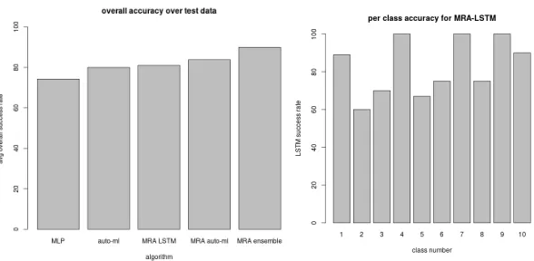
Figure 9, we plot the average accuracy over a 320/80 split (recorded over 5 runs) for a Multi-Layer Perceptron, MRA LSTM, MRA auto-ml, and MRA ensemble approaches. We observe significant accuracy improvements with the MRA approach.

5

Conclusion

Figure 9: Overall accuracy results (one alg: MLP, auto-Weka on untransformed signal features), MRA LSTM,

MRA auto-Weka, and MRA ensemble (auto-Weka + LSTM) on multiple feature sets, MRA LSTM by class results.

References

[1] Maxime Baelde, Christophe Biernacki, and Rapha¨el Greff. A mixture model-based real-time audio sources classification method. In Acoustics, Speech and Signal Processing (ICASSP), 2017 IEEE International Conference on, pages 2427–2431. IEEE, 2017.

[2] Amina Chebira, Yann Barbotin, Charles Jackson, Thomas Merryman, Gowri Srinivasa, Robert F Murphy, and Jelena Kovaˇcevi´c. A multiresolution approach to automated classification of protein subcellular location images. BMC bioinformatics, 8(1):210, 2007.

[3] Sepp Hochreiter and J¨urgen Schmidhuber. Long short-term memory. Neural computation, 9(8):1735–1780, 1997.

[4] Josef Kittler, Mohamad Hatef, Robert PW Duin, and Jiri Matas. On combining classifiers. IEEE transac-tions on pattern analysis and machine intelligence, 20(3):226–239, 1998.

[5] Olivier Lartillot and Petri Toiviainen. A matlab toolbox for musical feature extraction from audio. In International Conference on Digital Audio Effects, pages 237–244, 2007.

[6] Guohui Li and Ashfaq A Khokhar. Content-based indexing and retrieval of audio data using wavelets. In Multimedia and Expo, 2000. ICME 2000. 2000 IEEE International Conference on, volume 2, pages 885–888. IEEE, 2000.

[7] Martin McKinney and Jeroen Breebaart. Features for audio and music classification. 2003.

[8] Derek Monner and James A Reggia. A generalized lstm-like training algorithm for second-order recurrent neural networks. Neural Networks, 25:70–83, 2012.

[9] Jean-Baptiste Monnier et al. Classification via local multi-resolution projections. Electronic Journal of Statistics, 6:382–420, 2012.

[10] Karol J Piczak. Environmental sound classification with convolutional neural networks. InMachine Learning for Signal Processing (MLSP), 2015 IEEE 25th International Workshop on, pages 1–6. IEEE, 2015.

[11] Karol J Piczak. Esc: Dataset for environmental sound classification. In Proceedings of the 23rd ACM international conference on Multimedia, pages 1015–1018. ACM, 2015.