Vol 2, No 2, pp. 145–152, 2010 AVAILABLE ONLINE AT HTTP://MCFNS.COM Submitted: Jan. 1, 2010
International Journal of Accepted: Jun. 16, 2010
Mathematical and Computational Published: Aug. 28, 2010
Forestry & Natural-Resource Sciences Last Correction: Aug. 26, 2010
EVALUATING TIFFS (TOOLBOX FOR LIDAR DATA FILTERING
AND FOREST STUDIES) IN DERIVING FOREST
MEASUREMENTS FROM LIDAR DATA
John Chapman
1, I-Kuai Hung
2, Jeff Tippen
31Graduate Assistant,2Associate Professor, Stephen F. Austin State University, Nacogdoches, TX 75962 USA 3Senior Project Engineer, Surdex Corporation
Abstract. Recent advances in LiDAR (Light Detection and Ranging) technology have allowed for the
remote sensing of important forest characteristics to be more reliable and commercially available. Studies have shown that this technology can adequately estimate forest characteristics such as individual tree locations, tree heights, and crown diameters. These values are then used to estimate biophysical properties of forests, such as basal area and timber volume. This study assessed the capability of a commercially available program, Tiffs (Toolbox for Lidar Data Filtering and Forest Studies), to accurately estimate forest characteristics, as compared to data collected at the plot level using traditional timber sampling methods. We found a high, positive correlation coefficient (r)of 0.8223 for tree heights, between the LiDAR-derived measurements and the field measurements, which is somewhat promising. However, we found low correlations in tree count per plot (r = 0.1777) and tree crown radius (r = 0.1517), be-tween the LiDAR-derived measurements and the field measurements, results which are far from satisfactory.
Keywords: LiDAR, remote sensing, forestry
1
Introduction
Remote sensing is an alternative method for obtain-ing spatial information, as compared to field-based mea-surements, which can be highly accurate but are time intensive and costly (Hydeet al. 2006). Aerial photogra-phy and satellite imagery have been implemented as re-mote sensing techniques for decades; however, they may require time-consuming and labor-intensive photogram-metric processes (Hyde et al. 2006). Further, these processes produce only two-dimensional images, with-out the resolution and accuracy sufficient for obtaining three-dimensional information for vegetation (Omasaet al. 2007, Lefksyet al. 2002). Alternatively, LiDAR sys-tems directly measure not onlyxandycoordinates, but
z coordinates as well, increasing the accuracy of mea-surements and extending spatial analysis into the third dimension (Lefsky et al. 2002).
LiDAR (Light Detection and Ranging) is an innova-tive remote sensing tool that essentially measures dis-tance with a laser. Disdis-tance is determined by measuring the travel time between an emitted and received pulse of light (Wehr and Lohr 1999). The travel time is the amount of time that elapses between the emission of a
light pulse, the reflectance of that pulse off of an object, and its recovery by the sensor (Wehr and Lohr 1999; Lim et al. 2003). These near-infrared laser pulses can be emitted at a high rate, exceeding 100,000 per second (Reutebuch et al. 2005, Evanset al. 2006). The pulse rate for the LiDAR system used in this study was 150 kHz. This technology is mounted to an aircraft in com-bination with an oscillating deflecting mirror to divert the beam to produce a wide-scan range and a Position and Orientation System (POS) to determine the loca-tions of reflective surfaces (Wehr and Lohr 1999). The POS consists of a differential Global Positioning System (dGPS) that extrapolates the position of the sensor, and an Inertial Measurement Unit (IMU) to account for roll, pitch, and yaw in the aircraft (Wehr and Lohr 1999, Lim et al. 2003, Simardet al. 2003, Evans et al. 2006). The result is a set of points that give the horizontal and verti-cal position of each recorded return in Earth-referenced coordinates (Evanset al. 2006). This is also referred to as a point cloud. Wehr and Lohr (1999) provided a more in-depth exploration into how LiDAR systems work.
Several different systems are currently available to ob-tain LiDAR data, and new methods for processing the data, particularly software, are being implemented
ev-Copyright c2010 Publisher of the International Journal ofMathematical and Computational Forestry & Natural-Resource Sciences
Figure 1: Location of the SFA Experimental Forest with color-infrared imagery.
ery day. With so many combinations of data acquisition and analysis, results of obtaining forest characteristics tend to vary. In the past, LiDAR was used mainly for terrain analysis and any returns of above-ground objects or trees were considered unwanted noise. Reutebuch et al. (2005) called for specifications and standards for Li-DAR missions to allow for optimal remote sensing for not just terrain, but vegetation as well. As these standards are being implemented, studies need to be designed to evaluate the effects they have on accuracy.
The recent advances in LiDAR applications have al-lowed for the remote sensing of important forest char-acteristics to be increasingly accurate, affordable, and commercially available. Studies have shown this tech-nology to be feasible in obtaining enough information to adequately estimate biophysical properties of forests, in-cluding stand volume and basal area (Meanset al. 2000). Traditionally, these properties are estimated from field measurements, which are costly and time intensive to obtain, or 2-dimensional image processing, which allows one to estimate area but not volume. With LiDAR, these types of forest measurements can be captured re-motely from a 3-dimensional perspective.
The purpose of this study is to provide some insight into the current capability of a commercially available software program, Toolbox for LiDAR data Filtering and Forests Studies (Tiffs). Tiffs is a product of Global-idar and it uses small-footprint LiDAR to estimate for-est characteristics. The objective is to evaluate the
cor-relation between LiDAR measurements and field mea-surements. Thus the evaluation was performed using an accuracy assessment that compared the LiDAR-derived measurements from Tiffs against field samples obtained with conventional methods.
2
Methods
2.1 Study Area and LiDAR Data Acquisition
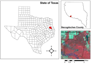
The study area is the Stephen F. Austin (SFA) Exper-imental Forest in Nacogdoches County, Texas, part of the Angelina National Forest. It was established by the U.S. Congress on December 14, 1944 and transferred to the U.S Forest Service for the purpose of cooperating with forestry-related research conducted by Stephen F. Austin State University (Russell 2002). The area con-sists of roughly 1,036 ha (2,560 acres) along the Angelina River, composed of southern bottomland hardwoods, southern pine, and mixed pine-hardwood forests. The elevation ranges from 53 to 80 m (173 to 263 ft) above mean sea level (Figure 1).
In cooperation with Stephen F. Austin State Uni-versity, the Surdex Corporation conducted a LiDAR flight mission over the SFA Experimental Forest. The data were obtained on August 15th, 2007, using a
Chapman et al. (2010)/Math. Comput. For. Nat.-Res. Sci. Vol 2, No 2, pp. 145–152/http://mcfns.com 147
250 m.
Figure 2: FIA (Forest Inventory and Analysis) plot lay-out.
2.2 Hardware and Field Measurement For
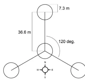
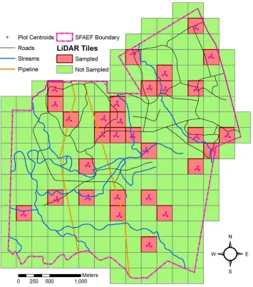
sam-pling purposes, the entire SFA Experimental Forest was divided into 205 tiles, 250 by 250 m each, correspond-ing to the grid system of the LiDAR dataset. Each tile was classified as either pine, hardwood, or mixed forest as the result of a majority process run against a digital land cover map for a four-county study in east Texas. The land cover map used for forest cover type classifica-tion of the tiles had an overall accuracy of 72.78%, and was derived from 30 m resolution Landsat ETM+ im-agery (Ungeret al. 2008). Thirty of these tiles were ran-domly selected, and stratified between the different cover types, with the primary focus on pine. Eleven tiles were selected from hardwood forests, fifteen from pine forests, and four from mixed forests. At the center of each tile, a plot was installed based on the sampling method out-lined by the USDA Forest Inventory and Analysis (FIA) National Program. A FIA plot consists of four circu-lar subplots; a center subplot and three subplots 36.6 m away from the center, 120o apart (Figure 2). Each
circular subplot has a radius of 7.3 m (Burkman 2005). For field data collection, a map of the study area was created with ArcGIS, and contained reference data such as roads, streams, and imagery (Figure 3). The map also contained the LiDAR tiles and a layer that contained the measured tree data. This map, along with its data, was transferred to a Trimble Recon handheld unit where data was entered in the field with the assistance of Arc-Pad software. With a Trimble Pro-XR GPS receiver, all trees with a DBH greater than 15.24 cm (6 inches) were mapped using the UTM coordinate system, NAD 1983. The height of each tree was measured using a Trupulse 200B rangefinder from Laser Technology Inc. Tree crown radii in the four cardinal directions (N, S, E, W) were
also measured with the rangefinder by positioning the unit underneath the edge of the crown and measuring the physical distance back to the tree trunk. Diameter at breast height (DBH) was measured using a diameter tape. For each tree measured, its status (alive or dead), species (generalized between pine and hardwood), and the date of data collection were recorded. To assist in the use of the rangefinder, and to provide greater ac-curacy, a retro-reflector surveyor’s prism mounted on a staff was used. A staff-compass was used to determine the locations of the sub-plots within each plot. The data collection was performed between May 2008 and May 2009. A total of 603 trees were measured.
2.3 Data Processing Tiffs (Toolbox for LiDAR
Data Filtering and Forest Studies) is a commercially available software program that uses an automated extraction process to generate digital surface models (DSM), digital elevation models (DEM), and canopy or object height models (CHM/OHM) based on Li-DAR data input (Chen 2007). The DSM is a raster layer that represents the elevation of the canopy. The DEM provides the elevation surface of the LiDAR re-turns that the software has deemed ground-rere-turns, de-picting the bare-earth terrain. The software then sub-tracts the DEM from the DSM to generate the CHM, which represents the height of the canopy above the bare ground. Tiffs then uses the CHM to isolate individual trees using a marker-controlled watershed segmentation method, and provides their location, height, and crown diameter (Chen et al. 2006, Chen 2007). This process was performed on each of the 30 randomly selected data tiles, and all LiDAR return values were used.
Other than generating DSM, DEM, and CHM in raster format, Tiffs also created a text file containing height, crown diameter, and thex,y, andzcoordinates of each individual tree identified in each data tile. The text files were converted to ESRI point shapefiles con-taining all trees and their associated attributes. The LiDAR-derived trees that fell within the boundary of the sample plots were selected and extracted for com-parison against the field-measured tree data. A total of 1,541 trees that were derived from the LiDAR were within the sample plots.
er-Figure 3: Map of the SFA Experimental Forest used for field data collection.
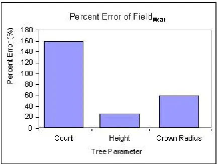
ror (Figure 4). The correlation coefficient, orr-statistic, was calculated between the LiDAR-derived and the field-measured measurements. In general, the higher the cor-relation coefficient, more accurate the LiDAR data es-timation process. Both the RMSE and the correlation coefficient (r) were calculated at the plot and sub-plot level using both unfiltered data and filtered data. The filtered data were obtained by removing field-measured trees that were classified as dead and having no crown to measure. Since trees with a DBH of less than 15.24 cm (6 inches) were not measured in the field plots, LiDAR-derived trees with height less than 7 m were removed from the analysis, with the assumption that trees less than 7 m tall would have a DBH of less than 15.24 cm (6 inches). This threshold was determined based on the correlation between tree height and DBH from the field-measured data.
3
Results and Discussion
Chapman et al. (2010)/Math. Comput. For. Nat.-Res. Sci. Vol 2, No 2, pp. 145–152/http://mcfns.com 149
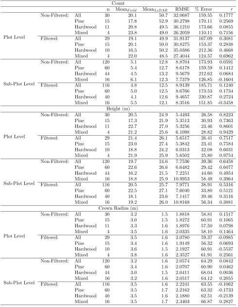
Table 1: Comparison of forest measurements between LiDAR-derived and field-measured data. Count
n MeanF ield MeanLiDAR RMSE % Error r
Plot Level
Non-Filtered: All 30 20.1 50.7 32.0687 159.55 0.1777
Pine 15 17.8 52.9 30.2798 170.11 0.2569
Hardwood 11 20.8 49.5 36.1210 173.66 0.0855
Mixed 4 23.8 49.0 26.2059 110.11 0.7156
Filtered: All 29 19.1 49.9 31.9137 167.09 0.3081
Pine 15 20.1 50.0 30.8275 153.37 0.2838
Hardwood 10 16.5 50.2 35.0386 212.36 0.4668
Mixed 4 22.0 48.5 27.4044 124.57 0.6962
Sub-Plot Level
Non-Filtered: All 120 5.1 12.8 8.8704 173.93 0.0591
Pine 60 5.4 12.7 8.6178 159.59 0.1412
Hardwood 44 4.5 13.2 9.5679 212.62 0.0684
Mixed 16 6.1 12.3 7.7379 126.85 -0.1604
Filtered: All 116 4.8 12.5 8.9139 185.71 0.1240
Pine 60 5.0 12.5 8.6766 173.53 0.1734
Hardwood 40 4.1 12.6 9.4657 230.87 0.2724
Mixed 16 5.5 12.1 8.3516 151.85 -0.3458
Height (m)
Plot Level
Non-Filtered: All 30 20.5 24.9 5.4493 26.58 0.8223
Pine 15 17.3 21.9 5.3513 30.93 0.7363
Hardwood 11 22.7 27.0 5.3256 23.46 0.8601
Mixed 4 21.2 25.6 6.1098 28.82 0.9429
Filtered: All 29 21.4 26.1 5.6517 26.41 0.7517
Pine 15 23.0 27.4 5.3842 23.41 0.7584
Hardwood 10 18.8 24.2 6.0313 32.08 0.6031
Mixed 4 21.9 25.9 5.6502 25.80 0.9754
Sub-Plot Level
Non-Filtered: All 120 19.7 24.6 7.7536 39.36 0.6458
Pine 60 22.6 26.6 6.6482 29.42 0.6077
Hardwood 44 16.2 21.5 7.2251 44.60 0.4954
Mixed 16 18.8 25.9 10.9953 58.49 0.3964
Filtered: All 116 20.5 25.7 7.9771 38.91 0.5316
Pine 60 22.5 27.1 7.6040 33.80 0.5121
Hardwood 40 18.1 23.6 7.1417 39.46 0.3116
Mixed 16 19.2 26.0 10.8168 56.34 0.3881
Crown Radius (m)
Plot Level
Non-Filtered: All 30 3.2 1.5 1.8818 58.81 0.1517
Pine 15 3.0 1.5 1.8272 60.91 0.1065
Hardwood 11 3.3 1.6 1.8976 57.50 0.0798
Mixed 4 3.5 1.6 2.0335 58.10 0.1464
Filtered: All 29 3.5 1.6 2.0780 59.37 -0.0985
Pine 15 3.4 1.6 1.9149 56.32 0.0693
Hardwood 10 3.6 1.5 2.1927 60.91 -0.5537
Mixed 4 3.8 1.6 2.3527 61.91 0.2561
Sub-Plot Level
Non-Filtered: All 120 3.2 1.6 2.0574 64.29 0.0842
Pine 60 3.4 1.6 2.0707 60.90 0.0462
Hardwood 44 3.0 1.5 2.0411 68.04 0.0036
Mixed 16 3.2 1.6 2.0517 64.12 0.2055
Filtered: All 116 3.5 1.6 2.2241 63.55 -0.1062
Pine 60 3.5 1.7 2.2162 63.32 -0.1733
Hardwood 40 3.5 1.6 2.1880 62.51 -0.2139
Figure 4: Comparison of percent error among tree pa-rameters based on the field mean.
be misidentified as an individual tree. The low correla-tion between the LiDAR-derived and the field-measured data for identifying trees also poses a problem when es-timating the timber volume of a stand. Unfortunately, the Tiffs program offered limited functionality for cali-bration.
For tree heights, the correlation using all trees at the plot level was relatively high (r = 0.8223) (Table 1, Height). When focusing on specific forest types, the r -values were 0.7363, 0.8601, 0.9429 for pine, hardwood, and mixed forests, respectively. For comparison pur-poses, Meanset al. (2000), in their study of Douglas-fir in the western Cascades of Oregon, were able to achieve anr-value of 0.96 (R2= 0.93) by using the average of the maximum heights of each 10 m grid cell when comparing LiDAR-derived tree heights to field-measured heights. Kwak et al. (2007), applied additional transformations to the watershed transformation as the basis for individ-ual tree delineation, and obtained anr-value of 0.88 (R2 = .77) for Korean pine trees in Central South Korea. Holmgrenet al. (2003) created an interpolated surface of the LiDAR data to obtain vertical distance from the estimated ground elevation, and then used local maxima to obtain mean tree heights. In their study, anr-value of 0.95 (R2= 0.90) was achieved.
For our study, the correlation in tree height is fairly consistent with the findings from other studies men-tioned above. However, the accuracy is still problem-atic when examining the RMSE of 5.4493 m (26.58%) when all trees were considered at the plot level (Table 1, Height). When comparing average tree height per plot, LiDAR-derived tree heights was greater than field-measured heights at all levels. This can be explained in that LiDAR detects tree heights based on the highest point of the canopy height model, whereas the tallest
point of a tree is usually difficult to see when measuring it in the field. Another possible cause is that LiDAR identified much larger number of trees than what was found in the field, which may bias the analysis towards higher values of the canopy. Traditionally, foresters mea-sure merchantable height in timber cruise. If LiDAR is to complement field measurements by identifying indi-vidual trees, the tree height measurement needs to be calibrated carefully.
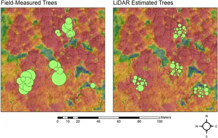
As for tree crown radius, the correlation coefficient for all trees at plot level was 0.1517, which is less than satisfactory (Table 1, Crown Radius). When examining specific forest types, the r-values were 0.1065, 0.0798, and 0.1464 for pine, hardwood, and mixed forests, re-spectively. When comparing the mean crown radius per plot, the LiDAR-derived measurements were always less than the field measurements. This problem is related to the fact that LiDAR identified more trees than what were found in the field. It is clear that LiDAR picked up more trees with limited overlapping crowns, while in re-ality there were actually fewer trees with larger crowns, which were often overlapping (Figure 5). This could be due to over-segmentation on the canopy height model when detecting individual trees (Kwaket al. 2007).
We also noticed that ther-value for the mixed forest type is greater than those of pine and hardwood for both tree count (r = 0.7156) and tree height (r = 0.9429) at the plot level (Tables 1, Count and Height). As tree detection is based on a continuous canopy height surface, the less homogeneous surface of the mixed forest allows for more accurate delineation of individual trees than those in pine and hardwood forests, which are generally more uniform in canopy structure.
4
Conclusions
While Tiffs estimation of tree height is promising, with a correlation coefficient of 0.8223, tree count and crown radius estimates appeared to be much less accu-rate. However, there was some consistency in the errors. Tiffs tends to overestimate the number of trees and un-derestimate the crown radius. Tiffs is an easy-to-use and affordable tool capable of analyzing LiDAR data, generating a DEM and a CHM, and also delineating in-dividual trees with their attributes. All of these outputs are useful in describing the structure of a forest stand. However, the software lacks the ability of allowing the user to calibrate the process in order to increase accu-racy.
an-Chapman et al. (2010)/Math. Comput. For. Nat.-Res. Sci. Vol 2, No 2, pp. 145–152/http://mcfns.com 151
Figure 5: Crown radius comparison of field-measured trees and LiDAR-estimated trees.
other. As a commercially available LiDAR data pro-cessing program, it should be made clear what types of landscapes will work best with the software. In the meantime, allowing for the calibration of estimates in conjunction with field-measured training data would in-crease the accuracy. If a forest manager is to choose a LiDAR data processing software program for opera-tional purposes, the ability to fine-tune the results is a criteria that should be considered in addition to the cost of the software.
acknowledgements
The authors would like to thank the U.S. Forest Ser-vice for granting access to the SFA Experimental Forest. We appreciate the four anonymous reviewers for their invaluable comments and suggestions. This project was partially funded by the U.S. National Park Service and by the McIntire-Stennis grant.
References
Burkman, B. 2005. Forest inventory and analysis sam-pling and plot design. FIA Fact Sheet Series. Available at: http://fia.fs.fed.us/library/fact-sheets/data-collections/Sampling%20and%20Plot%20Design.pdf. Accessed on September 6, 2009.
Chen, Q. 2007. Airborne lidar data processing and infor-mation extraction. Photogrammetric Engineering & Remote Sensing. 73(2):109-112.
Chen, Q., D. Baldocchi, P. Gong, and M. Kelly. 2006. Isolating individual trees in a savanna woodland us-ing small footprint lidar data. Photogrammetric En-gineering & Remote Sensing. 72(8): 923-932.
Evans, D. L., S. D. Roberts, and R. C. Parker. 2006. Lidar – a new tool for forest measurements? The Forestry Chronicle.82(2):211-218.
Holmgren, J., M. Nilsson, and H. Olsson. 2003. Esti-mation of tree height and stem volume on plots using airborne laser scanning. Forest Science. 49(3):419-428.
Hyde, P., R. Dubayah, W. Walker, J. B. Blair, M. Hofton, and C. Hunsaker. 2006. Mapping forest struc-ture for wildlife habitat analysis using multi-sensor (LiDAR, SAR/InSAR, ETM+, Quickbird) synergy. Remote Sensing of Environment. 102(1-2):63-73.
Lefsky, M. A., W. B. Cohen, G. G. Parker, D. J. Hard-ing. 2002. Lidar remote sensing for ecosystem studies. BioScience. 52(1):19-30.
Lim, K., P. Treitz, W. Cohen, and M. Berter-retche. 2003. Lidar remote sensing of forest structure. Progress in Physical Geography. 27(1):88-106.
Means, J. E., S. A. Acker, B. J. Fitt, M. Renslow, L. Emerson, and C. J. Hendrix. 2000. Predicting for-est stand characteristics with airborne scanning li-dar. Photogrammetric Engineering & Remote Sens-ing. 66(11):1367-1371.
Omasa, K., F. Hosoi, and A. Konishi. 2007. 3D lidar imaging for detecting and understanding plant re-sponses and canopy structure. Journal of Experimen-tal Botany. 58(4):881-898.
Reutebuch, S. E., H. E. Anderson, and R. J. Mc-Gaughey. 2005. Light detection and ranging (lidar): an emerging tool for multiple resource inventory. Jour-nal of Forestry. 103(6):286-292.
Russell, C. C. 2002. An early history of the Stephen F. Austin Experimental Forest: utilizing interactive multimedia and oral histories. MS thesis, Stephen F. Austin State University, Nacogdoches, Texas.
Simard, R., P. Belanger, M. R. Mohamed, and M. A. Othman. 2003. Airborne lidar surveys – an economic technology for terrain data acquisition. In: Proceed-ings of the Map Asia Conference 2003; 2003 Oct 13-15; Putra World Trade Centre, Kuala Lumpur, Malaysia. GISDevelopment.net.
Unger, D., J. Kroll, I-K. Hung, J. Williams, D. Coble, and J. Grogan. 2008. A standardized, cost-effective, and repeatable remote sensing methodology to quan-tify forested resources in Texas. Southern Journal of Applied Forestry. 32(1):12-20.