Image Segmentation of Printed Fabrics with Hierarchical Improved Markov Random Field in the Wavelet Domain

(1)

Image Segmentation of Printed Fabrics with Hierarchical

Improved Markov Random Field in the Wavelet Domain

Junfeng Jing, Qi Li, Pengfei Li, Hongwei Zhang, Lei Zhang

Xi`an Polytechnic University, Xi'an, Shaanxi CHINA

Correspondence to:

ABSTRACT

An improved MRF algorithm–hierarchical Gauss Markov Random Field model in the wavelet domain is presented for fabric image segmentation in this paper, which obtains the relation of inter-scale dependency from the feature field modeling and label field modeling. The Gauss-Markov random field modeling is usually adopted to feature field modeling. The label field modeling employs the inter-scale causal MRF model and the intra-scale non-causal MRF model. After that, parameter estimation is the essential section in the inter-scale, enhancing modeling capabilities of the pixels partial dependency. Sequential maximum a posterior criterion is applied to achieve the results of image segmentation. Comparisons with other hybrid schemes, results are indicated that performance of the presented algorithm is effective and accurate, in terms of classification accuracy and kappa coefficient, for patterned fabric images.

Keywords: Image segmentation; Feature field modeling; Label field modeling; Parameter estimation

INTRODUCTION

Printed fabric image segmentation is a very important process in textile printing and dyeing. The segmentation quality directly affects precision and accuracy of cloth printing as well as the subsequent drawing. Generally, image segmentation refers to divide into the different regions of the image that has a special significance in the division [1, 2]. These areas have mutually disjoint features, which own to gray, color, texture and other characteristics of similar principles. Image segmentation is not only a key step from image processing to image analysis, but also a basic technology of machine vision. There are numerous algorithms for image segmentation with threshold value method, the segmentation method based on edge detection, segmentation method based on fuzzy set theory, based on the random field

method and other segmentation algorithms. Based on the Markov Random Field (MRF) model has attracted much attention in recent years [3, 4, 5, 6, 7, 8]. In this paper, the proposed scheme is hierarchical Gauss Markov Random Field model in the wavelet domain, to obtain given image segmentation results more accurately and reliably.

(2)

criterion can obtain the final segmentation result. Experimental results show that the proposed algorithm is effective for fabric image segmentation, with respect to classification accuracy and kappa coefficient.

The rest of the paper is organized as follow. Section 2 describes the hierarchical Markov random field model. Section 3 gives feature field modeling, which is employed wavelet transform and Gaussian Markov random field methods. Section 4 gives label field modeling, including pyramid and Potts model. Section 5 contains parameter estimation. Section 6 presents experiment procedure. Section 7 discusses the experimental results step by step, comparing the results of proposed algorithm with MRF scheme, WMRF scheme, HMRF scheme and HWMRF scheme. Final Section 8 is devoted to conclusions.

The acronyms used in the paper are listed in Table I.

TABLE I. Glossary.

HIERARCHICAL MRF MODEL

Assuming thatS=

{

1,2,,n

}

indicates the position of each pixel in the image Y={ }Ys s∈S stands for feature field. The image to be segmented is the samples of feature field, namely y=

{

y1,y2,,yn

}

. Supposing

thatX =

{ }

Xs s∈Sis label field, namelyX=

{

x1,x2,,xn

}

,

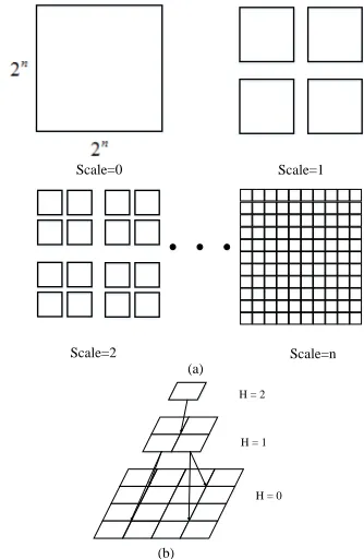
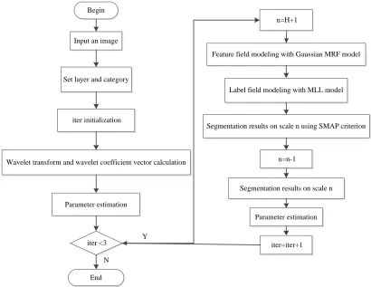
which represents segmentation result of the image. The basic framework of image segmentation is shown in

Figure 1. In this framework, it is assumed that the feature values of each pixel location are all dependent on the corresponding to each pixel of the label field. The corresponding category could be gotten. The labeled feature values are represented by the conditional probability density functionP

(

ys|xs

)

.

Label field is established by a causal hierarchical MRF model, [6, 12] as shown in Figure 2, which owns different resolutions and scales. Label field of

H

layers can be expressed as

X

=

{

X

0

,

X

1

,



,

X

H−1

}

.

0

X

indicates label field on the original resolution scales, and

X

n is label field on

n

−

th

scale. Pixel position set of the label field is denoted by

{

0

,

1

,

−1

}

=

S

H

S



on each scale. Each pixel

position of adjacent to the large scale corresponds to the four pixel positions on the current scale. Therefore, the size of grid position set

S

_n₋₁ is four times to the size of

S

_n.

FIGURE 1. The basic framework of image segmentation.

Scale=0 Scale=1

Scale=2 Scale=n (a)

H = 1 H = 2

H = 0

(b)

FIGURE 2. (a) Image divided into squares at different scales. Each square can be associated with Haar wavelet coefficients, (b) Hierarchical MRF model.

Acronyms Full Expressions

SMAP Sequential maximum a posterior

EM Expectation-maximization

MPL Maximum pseudo-likelihood

MLL Multi-level logistic

MRF Markov Random Field

WMRF Markov Random Field in the wavelet domain

HMRF Hierarchical Markov Random Field

HWMRF Hierarchical Markov Random Field in the wavelet domain

(3)

WAVELET TRANSFORM

To perform image segmentation based on wavelet domain MRF model, we have to make the wavelet decomposition for printed fabric image and select feature representation in every scale [13]. If a digital image

y

is defined in the grid

S

of the size of

N

×

,

H

+

1

layer wavelet decomposition of the image is denoted as

W

. Each of wavelet scale is represented by the corresponding level number

)

1

1 (

≤

n

≤

H

+

n

.

W

contains Np bands that are

respectively wavelet coefficients image

W

(b) (

b

∈

{

1 ,

2 ,



,

N

p

}

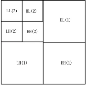
) of the wavelet transform. Each of

W

(b) structure is shown in Figure 3. The minimum resolution is

n

=

H

+

1

, which contains the wavelet coefficients of four bands

)

,

(

LL

LH

HL

HH

. Others resolutions are

)

1

1 (

≤

n

≤

H

+

n

, which correspond to the wavelet coefficients of three bands

(

LH

,

HL

,

HH

)

. Therefore, the wavelet coefficients that are each of resolution corresponding to bands of different position may be composed of vectors, forming the image corresponding to the vectors. The vectors used to express the image features in different resolutions. If the feature image that the layer number

n

=

0

regards as original resolution image, the feature sequence of the image of

H

resolutions is formed. The feature vector of minimum resolution scale

1 +

=

H

n

is shown as follow:

[

_n _N

]

T

ij b n ij n ij n ij n ij p

w

=

,(1)

,

,(2)

,



,

,( )

,



,

,( ) (1)

where,

[

, ,( ) ,,() , ,( ) ,,( )

]

) (

, _, _, _, HHn b

ij b n HL ij b n LH ij b n LL ij b n

ij w w w w

w = (2)

) ( , , ) ( , , ) ( , ,

,

_ijLHn b _ijHLn b

b n LL

ij

w

and

w

_ijHH,n,(b)

represent respectively the wavelet coefficients, which are the

b

−

th

band image and the position of each band

(

LL

,

LH

,

HL

,

HH

)

wavelet coefficients image (i, j) on

n

−

th

scale. But it doesn’t contain low frequency component. Eq. (2) could be improved as shown in Eq. (3).

[

, ,( ) , ,( ) , ,( )

]

) ( ,

,

ijHHn b

b n HL ij b n LH ij b n

ij

w

=

(3)

The size of each feature vector at the lowest resolution isD=4NP×1 and the size of the feature vector at the other resolutions isD=3NP×1.

FIGURE 3. Wavelet decomposition.

PARAMETER ESTIMATION

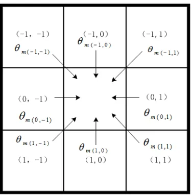
Improved Markov random field in the wavelet domain for printed fabric is proposed in this article, the appropriate parameters are estimated firstly for the feature field modeling and label field modeling. Feature field parameters are employed to obtain

n m n m n m

θ

(4)

FIGURE 4. Schematic of space interaction parameter.

The MPL method is used by estimating parameters of feature field. The parameters can be calculated by the following Eq. (4) through Eq. (8):

∑

∈

=

) )( ( ) , ( ) ( ) )( ( ) )( (

1

t n m L j i n ij t s m t n m

w

N

u

(4)

[

( ) ( ) ( )() ' '

]

) )( )( ( , 2 '

' _τ m τ η

τ + − ∈

= ₊ ₋ n t

m n ij n ij t n m

ij colw w

a (5)

              = ) )( )( ( ) )( )( ( ) )( )( ( ) )( )( ( 0 0 0 0 0 0 t n m ij t n m ij t n m ij t n m ij a a a A        (6)

(

)(

)

(

)(

)













×













=

∑

∈ − ∈ ( )() ₍_, ₎ ( )() ) )( )( ( ) )( )( ( 1 ) , ( ) )( )( ( ) )( )( ( ) )( ( t m m t m

m i j L

T t n m ij t n m ij L j i T t n m ij t n m ij t n

m

A

θ

(7)

[

][

_n _t

]

T

m T t n m ij n ij L j i t n m T t n m ij n ij t n m t n

m

w

A

w

A

N

n t

m ) )( ( ) )( )( ( ) ( ) , ( ) )( ( ) )( )( ( ) ( ) )( ( ) )( (

)

(

)

(

1

) )( (

θ

−

×

−

=

Σ

∑

∈ (8)

where,

m

is category, and

n

is the scale of

wavelet decomposition and

t

is iterations.

L

(_mn)(t)

stands for the set which is lattice position of labeled

m

on

n

−

th

scale n.

N

_m(n)(t) denotes the number of feature of labeled

m

on

n

−

th

scale.

(

) (

) ( )

{

1 ,

0 ,

1 ,

0 ,

1 }

'

=

−

η

is

second-order half-plane neighborhood.

Label field parameters contain

α

n

,

β

.

β

is a constant with experience, which will have an influence on the segmentation result. For instance, the smaller

β

, the less information about the spatial connection of the feature field will be obtained.

]

1 ,

0 [

∈

n

α

is interaction parameter of inter-scale. According to EM algorithm, that is:

(

)

(

) (

)

[

]

{

₁ ₁ '

}

, , | | , | ln max arg

ˆ n n n n n n

d n x w x x P y x w f E n α α α + +

= (9)

where,

α

n'is interaction parameter of inter-scale.

x

n is the scale for the wavelet vector

n

.

w

dn is the set of

wavelet coefficient vector

n s d

w

₍ ₎_.

PROPOSED ALGORITHM

(5)

First, the textile image begins with wavelet transform by using Haar wavelet [16].Then every pixel in the image turns into in the form of vector. According to these vectors, we could calculate likelihood value of vector corresponding to each location. We can represent the offset of neighborhood position relative

to the center position in the second-order neighborhood system with

τ

as shown in Figure 5, According to Gauss-MRF model [16-18], wavelet coefficients vector distribution on

n

−

th

scale is shown in Eq. (10):

(

)

_{( )}

( ) ( )













₋

_Σ

Σ

=

− n

s n m T n s n m B n s W s n

s

x

m

e

w

f

n ₁_/₂ 1

2

1 exp

2

1 ,

|

p

η

(10)

( ) (

) ( ) ( ) (

) (

) ( ) (

)

{

0 ,

1 ,

0 ,

−

1 ,

0 ,

1 ,

−

1 ,

−

1 ,

−

1 ,

−

1 ,

−

1 ,

0 }

=

∈

N

τ

B

is vector dimension. n

W s

η

is the set of the

second-order neighborhood corresponding to features of wavelet coefficients vector in the feature field on

th

n

−

scale.

x

n_s is the current labeled pixel.

e

_sn is

zero-mean noise vector at the position of

s

as

shown in Eq. (11):

(

n

)

m n s N n m n m n s n

s

w

e

m

θ

_τ

m

τ τ

−

×

−

=

₊ ∈

∑

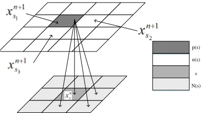
, (11)

In order to make full use of the inter-scale information, the neighborhood system should be

redefined as shown in Figure 5. The label of a node location is only relative to its parent node, uncle node and a second-order neighborhood nodes in this scale.

p(s)

u(s)

s

N(s)

FIGURE 5. Schematic of labeled position in the label field.

In Figure 5, considering that the location label of second-order neighbors has an effect in the current label, MLL model is employed [19-20]. The reason is that the location label of second-order neighbors is constantly updated in the iterative process. It is the non-causal intra-scale MRF model. Expression as shown in Eq. (12),

(

)

(

)

(

)

∑

     ₋      ₋ = ∈ + ∈ + s x N n s n s c N n s n s c n s N n s x x V x x V x x P τ τ τ τ | exp | exp | () (12)

where,

N

is the offset of second-order neighborhood location and the center location.

s

is the current node.

V

_c can be represented by Eq. (13).

(

)

₍

(

₎

)









≠

=

−

=

+ + + _n x n x n x n x n x n x

x

V

τ τ τ

_β

β

,

c (13)

where,

β

is a constant with experience.

(6)

{

(

|

,

)

(

|

,

)

}

max

arg

₍₎ ₍ ₎ ₍₎

^ s u s p n s n s s d x n s

x

P

w

x

w

f

x

n s

=













(14)













=

arg

max

(

|

,

)

(

|

(

)

₍ ₎

)

^ ) ( ^ n s N n s n s s d x n

s

f

w

x

w

P

x

n s (15)

]

)

,

|

(

)

,

|

(

[

)

,

|

(

)

,

|

(

) ( ) ( ) ( 1 1 ) ( ) ( 1

∏ ∑

∈ − − −

=

s c t x n t u n t p n t n t s d W s n s n s n s s d n t n

x

P

w

x

w

f

x

w

f

w

x

w

f

η

(16)

where,

s

is node, and

p

(

s

)

is father node, and

)

(

s

u

is uncle node.

N

(

s

)

is second-order

neighborhood node. In the process of image

segmentation on each scale, the marks of parent and uncle node transmits inter-scale marks, intermediate

result n s

x













^

is gotten. Then the marks of the

second-order neighborhood location optimize segmentation result on

n

−

th

scale, the final

segmentation result n s

x

^ is obtained. Experimental Procedure

The flow chart of proposed algorithm is shown in

Figure 6. The optimized segmentation result on scale n will be projected to scale

n

−

1

as the initial image for the new iteration. If the terminate condition,

that is, iter < 3, is not satisfactory, get back to repeat intra-scale and inter-scale iterations; otherwise,

stop the cycle and get the optimal segmentation result in the original resolution. The methods of hierarchical Gaussian MRF are summarized as

follow:

(1)

Feature field modeling. The wavelet transform is employed with Haar wavelet in fabric images firstly. Secondly, GMRF model is adopted to calculate conditional probability density

function.

(2)

Label field modeling. Potts and pyramid model are utilized to label the position of every pixel. Different positions of pixels in a fabric image are obtained in different scales.

(3)

Parameter estimation. Feature field parameters

include mn

n m n m

θ

m

,

Σ

,

with MPL method. Label

field parameters contain

α

,

β

with EM

algorithm. After that, SMAP criterion is applied to achieve the result of image segmentation for

(7)

Begin

Input an image

Set layer and category

iter initialization

Wavelet transform and wavelet coefficient vector calculation

Parameter estimation

iter <3

End

n=H+1

Feature field modeling with Gaussian MRF model

Label field modeling with MLL model

Segmentation results on scale n using SMAP criterion

n=n-1

iter=iter+1 Parameter estimation Segmentation results on scale n

Y

N

FIGURE 6. The flow chart of proposed algorithm.

RESULT AND ANALYSIS

We analyzed several types of fabric images so as to demonstrate the performance of our algorithm. Experiments are the Matlab compiling environment on personal computer with Intel 1.60 GHz processor and 1GB RAM. Fabric printing images with 256 × 256 DPI are contained by Canon 9000F scanner. It has been tested on multiple sets of experimental data to prove the effectiveness of the scheme. Parts of the typical segmentation results are selected to compare analyses from different angles.

(8)

(9)

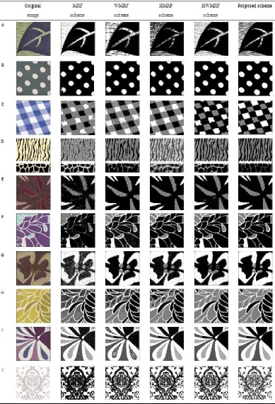
Figure 7 shows segmentation results of ten images by the proposed approach and other existing approaches. It can be shown that the proposed algorithm expresses image information comparatively better by reducing noise and solving problem of insufficient local spatial information statistics.

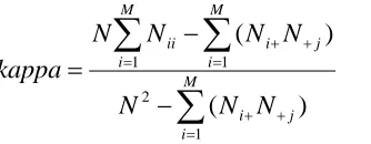
In current study, the equality of segmentation is weighted by visual effectiveness and quantitative indicators. Classification accuracy and kappa coefficient are calculated to measure segmentation effectiveness for fabrics, which represent the consistent probability of each random sample classification result and actual classification result. Overall classification performance is evaluated by two parameters, as shown in Eq. (17) and Eq. (18).

N

accuracy

tion

classifica

M

i ii

∑

=

1

(17)

∑

= + +

=

−

=

_M

i

j i M

i

j i M

i ii

N

kappa

1 2

1 1

)

(

)

(

(18)

where,

M

is the number of classification.

N

ij

represents the number of pixel that actual category

i

are classified as

j

.

N

shows the number of pixel.

∑

= +

=

M

j ij i

N

1

denotes the number of pixel that

classification results are divided into

i

−

th

category.

∑

=

+

=

M

i ij j

N

1

expresses the number of

pixel that

j

−

th

category is actually contained in

(10)

(a)

(b)

FIGURE 8. Curves of comparison with different methods, (a) classification accuracy of different schemes using 10 images, (b) kappa coefficient of different schemes using 10 images.

TABLE II. Average classification accuracy and kappa coefficient of five schemes.

Average Classification accuracy (%)

Average Kappa coefficient (%)

MRF scheme 60.33 48.37

WMRF scheme 80.87 73.20

HMRF scheme 82.28 74.73

HWMRF scheme 88.09 80.91

(11)

Figure 8 denotes the classification accuracy and kappa coefficient curves of comparison with different schemes using 10 images. Average classification accuracy and kappa coefficient of approaches are shown in Table Ⅱ. It can be concluded segmentation results by the above: in the realization of fabric image segmentation, the number of different images for classification, segmentation results accuracy of the MRF approach is 60.33%, and kappa coefficient reaches 48.37%. We can see the outline of fabric printing design, but there are lots of noises. In the implementation section of fabric image segmentation, the number of different images for classification, segmentation results accuracy of the scheme two is 80.87%, and kappa coefficient is 73.20%.Compared with the MRF scheme, the WMRF scheme can filter out some of the noise and describe the fabric edges and regional characteristics of the image. In the realization of the fabric image segmentation, the number of different images for classification, segmentation results accuracy of the HMRF method and HWMRF method is respectively to 82.28% and 88.09%. The kappa coefficient of them is respectively

to 74.73% and 80.91%. Compared with the previous two schemes, the HMRF and HWMRF algorithms could reduce noises and express spatial information accurately. Classification accuracy and kappa coefficient of proposed algorithm is to 94.03% and 88.28%. It can be demonstrated that this method filter out noise very perfectly, almost can accurately describe the fabric image edges and regional characteristics accurately. Experimental results show that proposed scheme can achieve a good segmentation performance for textile printing images.

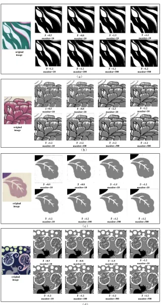
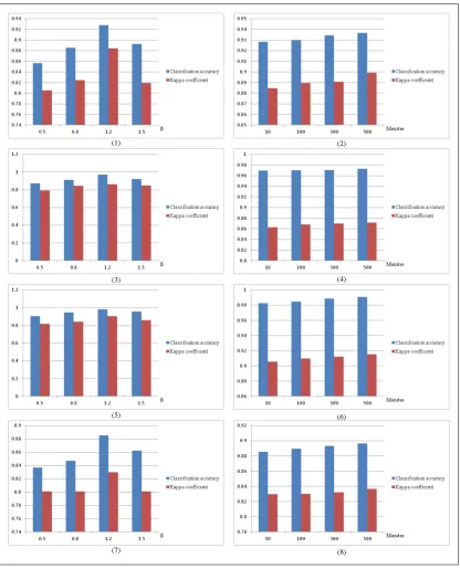
In proposed algorithm, there are two factors that affect the algorithm performance: the potential coefficient (β) and the number of iterations (max-iter). A comparison of classification accuracy and kappa coefficient with different β and max-iter is declared in Figure 9. The potential coefficient (β) plays a vital

(12)

β =0.8 maxiter=10

β =1.5 maxiter=10

β =1.2 maxiter=10

β =1.2 maxiter=100

β =1.2 maxiter=300

β =1.2 maxiter=500 β =0.5

maxiter=10

original image

β =0.5 maxiter=10

β =0.8 maxiter=10

β =1.5 maxiter=10

β =1.2 maxiter=10

β =1.2 maxiter=100

β =1.2 maxiter=300

β=1.2

maxiter=500 original

image

β =0.5 maxiter=10

β =0.8 maxiter=10

β =1.5 maxiter=10

β =1.2 maxiter=10

β =1.2 maxiter=100

β =1.2 maxiter=300

β =1.2 maxiter=500 original

image

β =0.5 maxiter=10

β =0.8 maxiter=10

β =1.5 maxiter=10

β =1.2 maxiter=10

β =1.2 maxiter=100

β =1.2 maxiter=300

β =1.2 maxiter=500 original

image

（c）

（d）（b）（a）

(13)

(1) (2)

(3) (4)

(5) (6)

(7) ₍₈₎

FIGURE 10. A comparison ofclassification accuracy and kappa coefficient using different parameters, (1)(2) by corresponding Figure 9(a), (3)(4) by corresponding Figure 9(b), (5)(6) by corresponding Figure 9(c), (7)(8) by corresponding Figure 9(d).

Histogram of classification accuracy and kappa coefficient to proposed algorithm is obtained in

Figure 10 (1)(3)(5)(7), when max-iter is 10 and β is

adopted different values. It can be concluded that the value of classification accuracy and kappa coefficient is higher than others, when β=1.2 and max-iter =10.

(14)

TABLE III. Evaluation parameters of proposed scheme.

β

(Maxiter=10)

0.5 86.79 80.42

0.8 89.77 82.84

1.2 94.15 87.02

1.5 90.88 83.17

TABLE IV. Evaluation parameters of proposed scheme.

Maxiter (β=1.2)

Time(s)

10 94.15 87.02 0.862

100 94.23 87.45 1.991

300 94.55 87.56 5.617

500 94.85 87.71 11.81

Table III indicates average classification accuracy and kappa coefficient of presented algorithm, when max-iter is 10 and β is applied different values. It can be concluded that average classification accuracy and kappa coefficient are able to achieve 94.15% and 87.02% respectively. Table Ⅳ declares the evaluation parameters of proposed scheme. When the number of max-iter is increasing, the results of image segmentation are improved in terms of average classification accuracy and kappa coefficient, and it has little effect. However, the higher the number of max-iter is, the longer time of the segmentation results would be. It would increase the cost in practice application. Therefore better result of image segmentation is achieved for fabrics when β employs 1.2 and max-iter is used 10.

CONCLUSION

In this paper, the traditional MRF model algorithm has been improved gradually and hierarchical GMRF in wavelet domain algorithm is proposed. In the process of the fabric image segmentation，it involves feature field modeling, label field modeling and parameter estimation. Feature field modeling is combination of wavelet transform and Gaussian MRF model algorithm. Label field modeling integrates MLL model to label the position of each pixel in fabric images. The interaction parameters are

employed by MPL and EM algorithm, calculating for the likelihood value of each scale and from coarse scale to fine scale in segmentation process.

The current status of research on image segmentation point of view, two aspects of the evaluation indicators of the quality of image segmentation is usually from the visual effects and quantitative analysis. From a visual point of view, it can be decided by the naked eye whether the marginal region consistent with the original image. Quantitative analysis of indicators is used in kappa coefficient and classification accuracy. This shows that proposed method can predict the image segmentation of fabrics with acceptable accuracy. In the parameter training, a different area in the image could be selected, but the area is not the same choice every time, the result is slightly different. However, the impact is not big. That how to ensure that the same area is chosen every time continues research should be researched for no difference in the segmentation result.

ACKOWLEDGEMENTS

(15)

REFERENCES

[1] Y. Boykov and G. Funka-Lea. Graph cuts and efficient n-d image segmentation. International Journal of Computer Vision 2006; 70(2):109-131.

[2] Shoba Rani, Dr. S. Purushothaman. Implementation of Textile Image Segmentation Using Rotational Gabor Filter and Echo State Neural Network. International Journal of Scientific and Engineering Research 2013; 4(5):457-462. [3] A. Shekhovtsov, I. Kovtun, V. Hlavac. Efficient

MRF deformation model for non-rigid image matching. Computer Vision and Image Understanding 2008; 112(1):91-99. [4] Chaohui Wang, Nikos Komodakis, Nikos

Paragios. Markov Random Field modeling inference & learning in computer vision & image understanding: A survey. Computer Vision and Image Understanding 2013; 117:1610-1627.

[5] Satoshi Sashida, Yutaka Okabe, Hwee Kuan Lee. Comparison of multi-label graph cuts method and Monte Carlo simulation with block-spin transformation for the piecewise constant Mumford-Shah segmentation model. Computer Vision and Image Understanding 2014; 119:15-26.

[6] Sahar Yousefi, Reza Azmi, Morteza Zahedi. Brain tissue segmentation in MR images based on a hybrid of MRF and social algorithms. Medical Image Analysis 2012; 16(4):840-848.

[7] Ricardo Omar Chavez, Hugo Jair Escalante, Manuel Montes-y-Gomez. Multimodal Markov Random Field for Image Re-ranking Based on Relevance Feedback. ISRN Machine Vision 2013.

[8] Rafal Zdunek. Improved Convolutive and Under-Determined Blind Audio Source Separation with MRF Smoothing. Cognitive Computation 2013; 5(4):493-503.

[9] Comer, M.L., E.J.Delp. Segmentation of textured images using a multi-resolution Guassian autoregressive model. IEEE Transaction on Image Processing 1999; 8(3): 408-420.

[10] Emmanouil A, Dionisis C and Spyros K. A wavelet-based Markov random field segmentation model in segmenting microarray experiments. Comput Meth Prog Bio 2011; 104(3):307-315.

[11] Bousse Alexandre, Pedemonte Stefano, Thomas Benjamin A. Markov random field and Guassian mixture for segmented MRI-based partial volume correction in PET. Physics in Medicine and Biology 2012; 57(20):681-705.

[12] O. Veksler. Multi-label moves for MRFs with truncated convex priors. International Journal of Computer Vision 2012; 98(1):1-14.

[13] K. Seetharaman, V. Rekha. Near-Lossless compression based on a full range Guassian Markov random field model for 2D monochrome images. Journal of Signal and Information Processing 2013; 4(01):10-23. [14] Stelios Zimeras. Modified maximum likelihood

estimation of the spatial resolution for the elliptical gamma camera SPECT imaging using binary inhomogeneous Markov Random Fields models. Advances in Computed Tomography 2013. 2(02):68-75. [15] Lee Anthony, Caron Francois, Doucet Arnaud.

Bayesian sacristy-path-analysis of genetic association signal using generalized priors. Statistical Applications in Genetics and Molecular Biology 2012; 11(2).

[16] H. Permuter, J. Francos, and I. Jermyn. A study of Guassian mixture models of color and texture features for image classification and segmentation. Pattern Recognition 2006; 39(4):659-706.

[17] Zhu Xijun, Wang Chuanxu. Unsupervised posture modeling and recognition based on guassian mixture model and EM estimation. Journal of Software 2011; 6(8):1445-1451. [18] Kevin Thon, Havard Rue, Stein Olav Shrovseth,

Fred Godtliebsen. Bayesian multiscale analysis of images modeled as Guassian Markov random fields. Computational Statistics and Data Analysis 2011; 56(1):49-61.

[19] Cressie, N., N. Verzelen. Conditional-mean least-squares fitting of Gaussian Markov random fields to Gaussian fields. Computational Statistics and Data Analysis 2008; 52(5) : 2794-2807.

(16)

[21] A. Lachkar, R. Benslimane, L. D'Orazio and E. Martuscelli. A system for textile design patterns retrieval. Part I: Design patterns extraction by adaptive and efficient color image segmentation method. Journal of the Textile Institute 2006; 94(4):301-312.

[22] K. Alahari, P. Kohli, P.H.S.Torr. Dynamic hybrid algorithms for MAP inference in discrete MRFs. IEEE Transactions on Pattern Analysis and Machine Intelligence 2010; 32(10):1846-1857.

AUTHORS’ ADDRESSES Jing Jun Feng

Pengfei Li Hongwei Zhang Lei Zhang