AN IMPROVED EVALUATION METHOD
FOR AVAILABLE TRANSFER
CAPABILITY BY INCORPORATING THE
REACTIVE POWER FLOWS
KIRAN SEELAM
Assistant Professor, Department of Electrical Engineering Malla Reddy Institute of Engineering & Technology,
Dhulapally, Hyderabad, India SURENDER KUMAR YELLAGOUD
Research Scholar, Department of Electrical Engineering, Jawaharlal Nehru Technological University,
Hyderabad, India
VEERANJANEYULU PUPPALA Associate Professor, Department of Electrical Engineering Malla Reddy Institute of Engineering & Technology,
Dhulapally, Hyderabad, India
Abstract - During the last decade electric power industry has undergone considerable changes. System operators
will need to be well-aware of the network capability to transfer. Various mathematical models have been developed to find Available Transfer Capacity (ATC) of transmission system. Most transfer studies Developed are based on linear methods. One of the limitations of linear ATC is the error produced by neglecting the effect of reactive power flows in line loading. This paper describes a fast algorithm to incorporate this effect. The estimation of the line post -transfer complex flow is based on circle equations and a Megavar-corrected Megawatt limit. The algorithm is illustrated with a small example.
Keywords: PTDF, Linear ATC, Reactive Power Flows, Line loading limits
I. INTRODUCTION
Available transfer capability (ATC) determines the ratings of the largest transfer system that can be implemented
in a certain direction across the power grid without violating security constraints. Mathematically ATC is defined as the Total Transfer Capability (TTC) less than both Transmission Reliability Margin (TRM) and also less than the sum of existing transmission commitments (which includes retail customer service and the Capacity Benefit Margin (CBM) by which ATC is actually considered as total transfer capability (TTC), while assuming that the other components related to ATC are zero for simplicity.
The determination of ATC requires the Power-flow, Steady-state stability, Voltage stability, and Transient stability simulations. The ATC study starts with a base case that corresponds to an initial operating point computed from a power flow solution using usual data specifications at PQ buses, PV buses, and a Slack bus. The transfer direction is of then specified by means participation factors of source and sink buses. In the simplest case, this would be a real power transmission to take place between bus s and bus t while holding all other power flow injections fixed at the base case levels.
a) Neglecting the nonlinear nature of real power flows; b) Ignoring reactive power flows.
c) Ignoring voltage levels.
This paper proposes an improved fast method that is between traditional linear methods and full nonlinear methods.
II. ATC CONVENTIONAL METHOD A .Linear static ATC
Based on the “dc” power flow model, linear ATC calculations typically assume a lossless system, where changes in the line real power flows are linearly related to changes in the net real power injections.
Consider a full fledged transfer from the slack bus ‘s’ to any bus ‘t’ and to maximize this transfer without exceeding the flow limits. The key to the linear power flow solution is the use of “power transfer distribution factors” (PTDF) expressed as sensitivities of line real power flows to bus injections. Power transfer distribution factors (PTDF) is expressed as
. Eq. (1)
These PTDFs can be determined as linearized sensitivities evaluated at the initial operating point. These used to predict the change in line flow (a-b) due to a transfer from (bus s-t) as,
∆
,∆
,∆
Eq. (2)Note that
∆
∆
is the amount of transferred power from s to t. For a given positive line flow limit ,assumed equal to the line MVA rating, and an initial positive line flow , the size of the transfer that drives the line to its limit is equal to
∆
.,
0
.
,
0
Eq. (3)
In order to determine ATC, the minimum value of
∆
in all lines in the system is determined. Note that it is the linear relation between the transfer and the line flows that makes linear ATC the fastest algorithm for transfer studies.
∆
:
Eq. (4) B. Line Complex Flows
Fig. 1 TRANSMISSION LINE MODEL
Consider the transmission line -model shown in Fig. 1.The complex power flow from bus to bus (at a) is
cos sin Eq. (5)
where,
,
are the voltage magnitudes and,
are the angles.is magnitude and is the angle of admittance
1/
)Now find the relation between the line active and reactive power flows as a transfer takes place across the system. Separating the real and imaginary components of (6) and re-arranging terms, we have
cos
Eq. (6)
sin
Eq. (7)Taking square of both sides and adding
Eq. (8)
are nearly constant during the transfer
i. e
VV VV0
Eq. (8) which is an assumption used in Linear ATC, the previous equation represents a circle in the plane , with center at
,
Eq. (9)and radius equal to Eq. (10) Here, denotes a constant circle parameter. Incorporating (9) and (10) into (8), we obtain,
Eq. (11)
Since, in general, the complex flow at the sending and receiving ends of a transmission line are different, there is a corresponding-end circle given by the equation.
Eq. (12)
where, in general, and
The radii of the two circles though have the same value. As the transfer increases, the flow in the line varies but all feasible operating points in the - - plane lie on the operating circle given by (11).The MVA rating of the line can be represented by a circle with center at the origin and radius equal to the thermal limit. This is referred to here as the limiting circle
Given an initial power system state without overloaded lines, the ATC calculation must determine the maximum amount for a transfer to such that the flows lie inside the limiting circle.
|
|
,
,
Fig. 2 General diagram of Operating circle, Limiting circle
III. INCLUSION OF REACTIVE FLOWS
Since the transmission line complex flow is constrained to be on the operating circle and inside the limiting circle, the maximum complex flow of the line - corresponds to point
,
By solving the above equations
Eq. (13)
Eq. (14)
Expand eq. (12) and subtracting eq. (13) we obtain the following,
2.
.
2.
.
Eq. (14)2.
.
Eq. (15)
where,
In order to get the value of substitute in the limiting circle equation we get the quadratic equation as,
. ′ . ′ 0
Eq. (16)
This is of the quadratic equation is of the form AX2+BX+C=0, then the roots of this equation are,
;
;
0;
√
;
Eq. (17)from the value of will be,
Eq. (18)
The sign in the previous equation is chosen to be positive if the PTDF of line - is positive and negative otherwise. In order to incorporate the maximum active flow in ATC, the only change required is to replace by . This differs from linear ATC where was assumedto be equal to MVA rating of the line. represents a better approximation to the actual maximum active line flow due to the transfer by considering the reactive power component.
The first step to determining is to obtain the circle parameters. These parameters are pre-transfer line flow solution. The values of M, A, B, C are constants during load flow. The method captures the behavior of reactive
power for large transfers and retains the use of active power distribution factors.
Note that given the base case power flow solution, the maximum active flow values are computed once and they remain constant during the ATC study. This is possible since the assumption of constant voltages, which is required in linear ATC, makes these values operating point and direction independent.
The process of computing linear ATC including the effect of reactive flows is summarized as follows. a) Compute distribution factors ,
b) Compute using (15) and (16);
c) Replace by and compute the necessary transfer
∆
to overload each line end using (3);d) Obtain the minimum
∆
among all line ends.IV. CASESTUDY
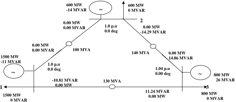
2
1 3
Fig. 3 IEEE 3 bus system
600 MW 0 MVAR 600 MW
-14 MVAR
0.00 MW 0.00 MVAR
800 MW 26 MVAR
1500 MW 0 MVAR 1500 MW -11 MVAR
800 MW 0 MVAR 1.0 p.u
0.0 deg 1.04 p.u
0.00 deg 100 MVA
130 MVA
140 MVA 1.0 p.u
0.0 deg
-10.81 MVAR 0.00 MW
11.24 MVAR 0.00 MW
0.00 MW
-14.29 MVAR
0.00 MW 0.00 MVAR
0.00 MW 14.86 MVAR
~
~
A. Simulation of a Small System
Consider the three-bus system in Fig. 3. The line reactance are 0.9, 0.37, and 0.28 p.u., and the line MVA ratings are 1.0, 1.3, and 1.4 p.u., for lines 1–2, 1–3, and 2–3, respectively. The initial operating point shown is set up with voltages equal to 1.0, 1.0, and 1.04 p.u. for buses 1, 2, and 3.Reactive power generation at every bus is unlimited. Transactions between areas 1 to 2, 1 to 3, and 2 to 3(seller/buyer) were simulated across this system. ATC was computed by three methods
a) Sequential full AC power flow, i.e., the actual ATC; b) Linear ATC, as described in Section II-A;
c) Linear ATC with reactive power flows, as described in Section III-A. Consider transfer from 1(seller) to area 3 (buyer) the limiting elements is again (3-1). B.Linear ATC Power Transfer Distribution Factors (PTDF)
Seller Bus: 1; Buyer Bus: 3;
Branch Number Sending Bus Receiving Bus PTDF
1 1 2 0.23329
2 1 3 0.76671
3 2 3 0.23329
C. Calculations
Branch Number
Branch Flow (MW)
Line Limit (MW)
PTDF LATC
(MW)
1 0.00 100.00 0.23 428.65
2 0.00 130.00 0.77 169.56
3 0.00 140.00 0.23 600.11
Limiting Branch : 2
Linear ATC (MW) : 169.56
D. Enhancement of Linear ATC Calculation (by incorporating reactive power flows)
Modified Line (2) flows by considering the line limit be ′ : 123.71 MW (taking reactive power flows):
Branch Number
Branch Flow (MW)
Line Limit (MW)
PTDF LATC
(MW)
1 0.00 100.00 0.23 428.65
2 0.00 123.71 0.77 161.36
3 0.00 140.00 0.23 600.11
Limiting Branch : 2 Modified Linear ATC (MW) : 161.36 V. RESULTS ANALYSIS
VI. CONCLUSION
The results obtained in this paper show that incorporating the effect of reactive power flows in transmission elements results in significant error reduction in linear ATC. The method is based on a Megavar- corrected megawatt limit, which captures the change in reactive power flow as the active power flow in the line increases due to large transfers.
VII. REFERENCES
[1] “NERC transmission transfer capability task force,” in Available Transfer Capability Definitions and Determination. Princeton, NJ: North American Electric Reliability Council, 1996.
[2] Enhancement of Linear ATC Calculations by the Incorporation of Reactive Power Flows Santiago Grijalva, Member, IEEE Peter W. Sauer, Fellow, IEEE, and James D. Weber, Member-IEEE, IEEE-TRANSACTIONS ON POWER SYSTEMS, VOL. 18, NO. 2, MAY 2003.
[3] Modern Power System Analysis 3rd Edition, D.P .KOTHARI, I .J NAGARATH.
[4] M.H.Gravener and C.Nwankpa, “Available transfer capability and first order sensitivity,” IEEE Trans. Power Syst., vol.14, pp.512–518, May 1999.
Test Cases with and without Reactive power flows inclusion
0 0.5 1 1.5 2 2.5 3
0 100 200 300 400 500 600 700 Li n e a r AT C va lu es at di ff er e nt bu se s
ATC without Q flows ATC with Q flows
1 2 0 100 200 300 400 500 600 700 Li ne a r AT C val u e s at di ffe re nt bu se
s ATC at bus 1
ATC at bus 2 ATC at bus 3