Determining whether the squashing factor, Q, would be a good indicator of reconnection in a resistive MHD experiment devoid of null points

November 21, 2019

Is the squashing factor,

Q, a good indicator of reconnection in a

resistive MHD experiment devoid of null points?

J. Reid

, C. E. Parnell

, A. W. Hood

, and P. K. Browning

1 _{School of Mathematics and Statistics, University of St Andrews, St Andrews, Fife, KY16 9SS, UK.}

2 _{Jodrell Bank Centre for Astrophysics, School of Physics and Astronomy, University of Manchester, Manchester, M13 9PL, UK.}

3 _{e-mail:[email protected], [email protected]}

21 November 2019

ABSTRACT

The squashing factor of a magnetic field,Q, is commonly used as an indicator of magnetic reconnection, but few studies seek to eval-uate how reliable it is in comparison with other possible reconnection indicators. By using a full, self-consistent, three-dimensional, resistive magnetohydrodynamic experiment of interacting magnetic strands constituting a coronal loop,Qand several different quan-tities are determined. Each is then compared with the necessary and sufficient condition for reconnection, namely the integral along a field line of the component of the electric field parallel to the magnetic field. Among the reconnection indicators explored, we find the squashing factor less successful when compared with alternatives such as Ohmic heating. In a reconnecting magnetic field devoid of null points, our work suggests thatQ, being a geometric measure of the magnetic field, is not, in some configurations, a reliable indicator of the onset or a diagnostic of the location of magnetic reconnection.

Key words. Sun: corona - Sun: magnetic fields - Magnetic reconnection - Magnetohydrodynamics (MHD)

1. Introduction

One of the key physical plasma processes that play a major role in dynamic events on the Sun, in other stars, in the magneto-sphere, and in laboratory experiments, is magnetic reconnection (Priest & Forbes 2000; Zweibel & Yamada 2016). It is a known driver of solar and stellar flares (e.g. Carmichael 1964; Sturrock 1966) (reviewed by, e.g., Pontin 2012), is likely to be involved in heating solar and stellar coronae, as well as accretion discs (e.g. Ross & Latter 2018), and also plays a role in dynamic ejecta, such as coronal mass ejections and jets (e.g. Archontis & Hood 2013; Raouafi et al. 2016). In the magnetosphere, the interac-tion and subsequent reconnecinterac-tion of the magnetic solar wind and the different connectivities of the Earth’s magnetic field, on both the dayside and the nightside, are important for triggering substorms, causing aurora and creating flux transfer events (e.g. Dungey 1961; Hones 1979; Wright 1987; Phan et al. 2016). Both large-scale plasma physics experiments, such as the International Thermonuclear Experimental Reactor (ITER) and the Joint Eu-ropean Torus (JET), and small-scale, such as the Small Tight Aspect Ratio Tokamak (START) and Mega Ampere Spherical Tokamak (MAST), involve reconnection (e.g. Stanier et al. 2013; McClements 2019), with, in several cases, the reconnection be-ing key to the initial creation of the isolated plasma.

In order to understand the behaviour of the plasma systems mentioned above, three-dimensional models are used. These models study either the complete system or a part of it, through potential or magnetohydrostatic (MHS) equilibria (e.g. Low 1985; Bogdan & Low 1986; Neukirch 1995), complex numerical MHD simulations (e.g. Galsgaard & Nordlund 1996; Bingert & Peter 2011), multi-fluid simulations (e.g. Yamada 2010), or particle-in-cell (PIC) experiments (e.g. Baumann & Nordlund 2012). In order to analyse reconnection in these systems, it is useful to determine the sites at which magnetic

reconnec-tion takes place. Over years, a host of different approaches have been employed, depending upon the modelling undertaken. When modelling involves only two-dimensional magnetic sys-tems, identifying the sites of reconnection is relatively straight-forward: these must be X-type null points, since, in two dimen-sions, these are the only locations at which reconnection can oc-cur, as discussed in detail by Priest & Forbes (2000). In three di-mensions, however, reconnection is much more varied, and may occur not only at a magnetic null points, but also away from such locations (Vasyliunas 1984; Schindler et al. 1988; Priest & Forbes 2000).

of the field line mapping are very large. Titov et al. (2002) adapt this definition to formulate the squashing factor,Q, and suggest that regions of highQare likely sites for reconnection. Recently, Boozer (2019) has emphasized the role of exponential separation of field lines in three-dimensional geometries in allowing for fast reconnection.

Since its conception, the squashing factor has seen exten-sive use as an identifier and measure of reconnection (as elab-orated by Janvier 2017). Longcope & Strauss (1994) illustrate the viability of the formation of electric currents on QSLs. In solar physics, its popularity is partly on account of its being in-ferable from magnetograms. The formation of electric currents and consequent capacity for reconnection have been noted in analytic models of QSLs (e.g. Titov et al. 2003) and on broad, pre-existing QSLs in numerical simulations (e.g. Galsgaard et al. 2003; Milano et al. 1999). Aulanier et al. (2005) find evidence of precisely such a connection between reconnection andQin specific steady, and so not time-dependent, configurations, and demonstrate narrow current layers more generally at QSLs. In the presence of null points, reconnection has been noted embed-ded within QSLs, where intense currents can accumulate (Mas-son et al. 2009). Maclean et al. (2009) find a relationshipQand

Ekin fields generated from magnetograms and subject to a slow

shearing. Moreover, De Moortel & Galsgaard (2006a,b) find ev-idence of rotating or spinning the footpoints of coronal loops leading to QSLs that are candidate sites for reconnection, and are associated with the creation of strong current layers, the pre-cise configuration of which is determined by the nature of the footpoint motions applied. It has, indeed, been argued that, al-though QSLs and strong currents need not be linked in general, they are more likely to occur together under the action of bound-ary motions (as argued by Tassev & Savcheva 2017). Modelling of such boundary motions introduces a new perspective, since they are typically treated in models between two parallel photo-spheric planes, which contrasts with the configuration in which the squashing factor was originally formulated, that assumed field lines mapping from one part to another of a single plane, across a polarity inversion line. However, the mathematical com-position remains identical. With particular regard to models of line-tied coronal flux tubes, the two conceived parts represent equally part of one single physical solar surface; their being par-allel removes additional effects caused by curvature.

Observations of solar phenomena provide evidence of such a link between squashing of the magnetic field and reconnection. Reconnection at QSLs or hyperbolic flux tubes (HFTs), along-side topological features, clearly occurs, providing some of the observed particle acceleration from ribbons and the associated strong emission (Reid et al. 2012). Indeed, the extrapolations of the fields around flares have shown high-Qregions without null points, giving strong evidence of their role in reconnection (e.g. Mandrini et al. 2006). Far more limited has been the exam-ination ofQwith respect to field-line-integrated parallel electric field,R Ekds. Maclean et al. (2009) demonstrate correlation of

the two in reconnecting fields with null points, although estab-lishing this visually and not quantitatively. Wilmot-Smith et al. (2009, 2010) find QSLs existing away from active sites of recon-nection, and argue that the nature of their relationship with re-connection is not clear, in line with the similar work of Restante (2011). Should it be possible to establish a link between the two, it has been suggested, in turn, to be a contributing factor for heat-ing and particle acceleration (Démoulin & Priest 1997; Aulanier et al. 2006). As discussed above, undoubtedly, QSLs are docu-mented to be able to host reconnection, and tentative evidence agrees that they may be then linked with the occurrence of

so-lar fso-lares (Démoulin et al. 1996a, 1997). Nevertheless, little in existing literature compares Q and R Ekds in a globally

non-null magnetic field. Wendel et al. (2013) find ‘excellent agree-ment’, in a kinetic simulation of generic reconnection, between the boundaries of quasi-potentialΞ = −R_α,βEkdsand the QSL.

In laboratory plasma, reconnection can occur at sites whereQis high and currents are created. QSLs exist in reconnecting labo-ratory flux ropes (Gekelman et al. 2010, 2012); likewise, Gekel-man et al. (2016) identify highQassociated with a reconnecting current sheet, yet remark even higher subsequent values ofQnot linked with any reconnection, suggesting that any relationship is subtle and complicated.

Whilst it has been previously often suggested that regions of highQare likely sites of reconnection in the presence of driving flows, no rigorous quantitative link has been established between

Qand reconnection locations. Here, for the first time, we provide a statistical analysis between the various potential indicators of reconnection, including Q and Ohmic heating. In order to in-vestigate this, it is necessary to use 3D MHD simulations, since both dynamics and three-dimensional fields are essential in or-der to have reconnection and forQto play a role. Similarly to the work of De Moortel & Galsgaard (2006a,b), we have considered reconnection within modelled coronal loops subject to boundary motions. We investigate the conditions in whichQforesees re-connection in braided magnetic fields arising from driving flows. We study the distribution of the localized instances of reconnec-tion and analyse their nature. Such forms of driven reconnecreconnec-tion are likely to contribute, at least in some measure, to the heating necessary in the solar atmosphere (Parnell & Galsgaard 2004).

In order to understand the locations of magnetic reconnec-tion, and the validity of different indicators of reconnection in fields of simple topology, without null points, we utilize the mag-netic field configuration studied in the previous paper, Reid et al. (2018) (hereafter, Paper I). This field begins with a simple con-figuration of initially straight field lines, which, under the action of simple and ordered boundary motions, develops a complex pattern of multiple instances of reconnection. Building on pre-ceding studies of the kink instability in coronal loops, which Browning et al. (2008) and Hood et al. (2009) showed capa-ble of triggering instability and subsequent release of magnetic energy, the model demonstrated the formation of fragmentary structures in current. Instability and reconnection then spread among neighbouring threads, as in the generalization to several strands of Tam et al. (2015) and Hood et al. (2016).

In section 2, we sketch the model studied here, and in sec-tion 3 the broad evolusec-tion. Then, in secsec-tion 4, we seek to anal-yse the onset and occurrence of reconnection in that numeri-cal experiment. In section 5, we determine and compare several prospective indicators of reconnection. Finally, we draw conclu-sions in section 6.

2. Set-up of numerical experiment

2.1. Numerical method

The dimensionless equations of fully three-dimensional magne-tohydrodynamics (MHD) were solved, using the Lare3d code (Arber et al. 2001):

Dρ

Dt = −ρ(∇ ·v), (1)

ρDv

Dt = j×B− ∇P+Fshock+Fvisc., (2)

DB

Dt = (B· ∇)v−B(∇ ·v)− ∇ ×(η∇ ×B), (3)

ρDε

Dt = −P(∇ ·v)+ηj

2₊

Qvisc., (4)

where ρis mass density, vplasma velocity, B magnetic field,

P gas pressure, Fshock the shock viscosities, Fvisc. a uniform

viscous force,η = 1/σthe dimensionless magnetic resistivity (given conductivity σ; the dimensionless vacuum permeability isµ0 = 1),ε = P/ρ(γ−1) the specific internal energy (where γ = 5/3 is the ratio of specific heats), j current density, and

Qvisc. the combined viscous heating. The uniform viscosity is

implemented with a Laplacian operator acting on velocity,

Fvisc.=µ∇2v, (5)

given coefficient of dynamic viscosity µ. The system’s vol-ume, of dimensions −3 ≤ x,y ≤ 3 and −10 ≤ z ≤ 10, was discretized on a computational grid of 5122_{×2048 cells.}

These non-dimensional forms for the equations follow from the specification of a normalizing length L0, mass density ρ0,

and magnetic field B0. Thus, there are reference Alfvén speed

vA = B0/ p

(µ0ρ0), Alfvén time tA = L0/vA, energy density

W0 = B2₀/µ0, current density j0 =B0/(µ0L0), and electric field

E0=B2₀/ √

µ0ρ0.

The boundary conditions inzwere a photospheric driving velocity and zero-gradient for the remaining quantities. The side boundaries were periodic for all quantities. In terms of the nor-malization discussed above, the initial conditions comprised a plasma of uniform density and specific internal energy,ρ = 1 andε=0.1, in a uniform vertical magnetic fieldB=1ez. There

were no null points, initially or at any time subsequently. The ini-tial plasma beta, 2/15, being less than unity, indicates that mag-netic forces dominate. The full configuration and parameters of the model are detailed in Paper I.

2.2. Driving velocity

The spatial form for the driver is provided by:

vφ=

      

v0_ar

1−r2

a2

3

r<a,

0 r≥a, (6)

which was applied at three points, (−2,0), (0,0), and (2,0), around which the radial coordinate,r, is locally defined, in re-gions of fixed radius a = 1. The coefficientv0, regulating the

speed of driving, was chosen such the threads are respectively driven with maximum speeds 0.02, 0.05, and 0.02.

2.3. Resistivity model

Realistic coronal magnetic Reynolds numbers are not presently computational viable, on account of the extremely short length scales that would then need to be resolved. In order to match the

near-ideal nature of a coronal plasma as closely as is possible, we used zero uniform (background) resistivity. However, in or-der to study reconnection, the electric field must be calculated, which precludes relying on numerical dissipation. Therefore, an anomalous resistivity was applied above a certain threshold on the magnitude of total current density, jcrit..

The resistivity was accordingly prescribed by

η= ( _η

0 j> jcrit.,

0 j≤ jcrit.. (7)

In order to determine an appropriate current threshold, an ex-periment was conducted with only numerical diffusion. Within that numerical experiment, the imposed driving motions created three twisted threads; in the most rapidly driven central thread, a kink instability formed, provoking reconnection and the on-set of avalanche-like behaviour. The threshold on current, jcrit.,

was chosen from there, such that, in the main experiment, the build-up of current during the initial linear phase of the evolu-tion should not be inhibited and the central thread would attain marginal instability prior to the onset of reconnection. The level chosen was jcrit. =5.0, and the anomalous resistivity was fixed

atη0=10−3.

Our chosen model makes both resistivity and, consequently, the parallel electric field highly localized, which is physically apt: resistivity is not uniform. Plasma physics experiments have found it to be enhanced within localized regions of strong cur-rent, where length scales are of the order of a few ion inertial lengths (Cairns 1985). Within such regions, micro-instabilities generate turbulence, which disrupts the flow of electrons and causes a rise of several orders of magnitude in resistivity. In gen-eral, in coronal plasma,ηis so low as to be negligible, and only under certain conditions, achieved in localized regions, does it reach a material level, here reflected by the anomalous ‘switch-on’. Equally, this anomalous resistivity is motivated by resem-bling, on a finite grid, the collapse, given hypothetically infinite resolution, of length scales to a level at which classical resistivity would act.

3. Dynamic evolution under continued driving

current sheets, recur. Thus, this experiment involves numerous reconnection events that occur on a wide range of scales, and continue unabated from approximatelyt =175 onwards. None of these events are associated with null points, separators, or other topological features, as all the field lines remain largely vertical throughout the experiment. Hence, this numerical exper-iment is an instructive scenario in which to consider the associ-ation between the squashing factorQ, other potential identifiers, and actual sites of reconnection.

4. Occurrence of magnetic reconnection

As discussed earlier, the resistivity of coronal plasma is, in gen-eral, very small everywhere except within highly localized re-gions. A necessary and sufficient condition to identify the loca-tion and occurrence of three-dimensional reconnecloca-tion is

Z

E·ds

= Z

Ekds ,

0, (8)

wheresparameterizes the distance along a field line (Schindler et al. 1988; Hesse & Schindler 1988).

Indeed,R Ekdsis, in fact, everywhere non-zero in a plasma,

since classical resistivity is very small but non-zero, even in re-gions of approximately ideal MHD. When stated to be non-zero, it is intended that this integral is significantly larger than it is on a field line threading only these near-ideal MHD regions (Parnell 2018).

The integral in Eq. (8) is calculated starting from the mid-plane (z=0), through which all field lines are assumed to pass. Starting pointsxi,yj,0

are uniformly distributed over the grid in that plane. From there, field lines are traced in both directions, both forwards and backwards, and the parallel electric field,Ek= ηjk (cf. Eq. (9) below), integrated along them. For each time, a

total of 5132field lines are integrated.

Contours ofR Ekds, calculated from these points in the

mid-plane, are shown in Fig. 1 for six times. Those for the first two times demonstrate the beginning of the reconnection associated with the initial kink instability in the central thread (t = 175, Fig. 1a) and its aftermath (t =200, Fig. 1b), when evidence of reconnection has spread throughout the central thread’s cross-sectional area. Fig. 1c att =225 shows evidence of reconnec-tion having extended to the right thread, which has become com-pletely engulfed by reconnection att =275. At this time, there is also evidence in the left-hand thread of reconnection, possi-bly triggered by a kink instability. This thread is then shown to be affected by reconnection across its entire cross-section, both by its instability and by the growing unstable region to its right (t = 325, Fig. 1e). The aftermath of the disruption of all three threads att = 400 (Fig. 1f) reveals that reconnection is over a wide-spread area, much larger than that covered by the driven region on the top and bottom boundaries. These reconnection events continue, although their spatial locations and properties change throughout the rest of the experiment.

Within the several snapshots in Fig. 1, there are regions of both positive and negative field-line-integrated parallel elec-tric field. These persist throughout the experiment, with the re-gions of negativeR Ekdsoriginating in the centre of the twisted

threads and the positive regions originating in the outer rings. It is clear that

R

Ekds

is larger in regions where R

Ekds>0 than

whereR Ekds<0, although the data show a comparable number

of points where the integral is positive and negative. By taking

the component of Ohm’s law parallel to the magnetic field,

Ek= B

B ·E=

B

B· −v×B+

1 σj

!

= _σ1 jk. (9)

Thus, the sign ofEkis dependent on the direction of the electric

current relative to the magnetic field. In the early phase of the experiment, the magnetic field in a single thread, in cylindrical coordinates, has a poloidal component of the same spatial form as the driving velocity and an axial component from the initial vertical field. It can be calculated using the ideal induction equa-tion:

B=−λB0

r a 1−

r2 a2

!3

eφ+B0ez, (10)

where

λ≈v0t

L , (11)

(cf. Paper I). The correction to thez-component isOλ2 . Asso-ciated with this magnetic field is a vertical electric current,

jz=−

v0B0t

aL 1− r2

a2 !2

1−4r

2

a2 !

, (12)

which changes sign at r = a/2. The kink instability forms a current sheet at the mode-rational surfacer=rm, where

m rm

Bφ+kBz≈0, (13)

(e.g. Bateman 1978; Hood & Priest 1979). Here,m = 1 is the mode number for the kink mode, and we considerk= ₂π_L as the axial wave number. Thus,

rm=a

s

1− 3

r _π

a

2Lλ. (14)

At marginal instability, we approximateλ = 1.586 (more fully discussed in Reid et al. 2018), which yieldsrm≈0.73>0.5.

Ac-cordingly, the current sheet associated with the kink instability emerges where the current is mainly in the positivez-direction. Hence, instability occurs whereEkis similarly positive.

Notwith-standing this, as is obvious in Fig. 1, reconnection does occur in whichEk<0, likely proceeding from reconnection after the kink

instability near the centres of threads, where parallel current is negative.

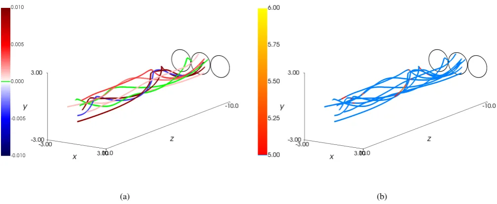
Fig. 2 shows, at timet=200, a sample of field lines in three dimensions, coloured according toR Ekds(Fig. 2a) and,

sepa-rately, according to the current along each field line (Fig. 2b). As expected in a plasma with a high magnetic Reynolds number, the current along a field line only breaches the threshold necessary to trigger reconnection in small, localized regions, and soR Ekds

is only non-zero in such confined regions. It is seen that strong current, associated with current layers, cannot be of great spatial extent, nor can it persist for long. The large magnitudes of cur-rent that form the curcur-rent layers are both small and short-lived, since the anomalous resistivity efficiently dissipates all such cur-rent. However, currents are continuously being build up through the twisting of the field via the driving motions.

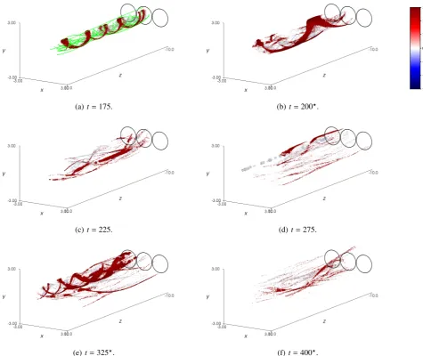
Similarly in three dimensions, the location at which recon-nection occurs is shown in Fig. 3 by isosurfaces of the parallel electric field, Ek, found locally within the domain. In Fig. 3a,

(a)t=175. (b)t=200?. (c)t=225.

­0.050 −2.924 × 10−4

−1.710 × 10−6

0.000 1.710 × 10−6

2.924 × 10−4

0.050

E∥

ds

 (E0 L0

)

(d)t=275. (e)t=325?. (f)t=400?.

Fig. 1.Contours of the field-line-integrated parallel electric field, plotted where field lines intersect the mid-plane. Times shown are (a)t=175, (b)t=200, (c)t=225, (d)t=275, (e)t=325, and (f)t=400. The starred times are subsequently considered in greater detail. In (a), the dashed black lines indicate the radii of the driven regions, representing footpoints of the left, central, and right threads. The contours are shaded according to the logarithmic scale on the colour bar.

(a) (b)

Fig. 2.Sample of field lines traced from the mid-plane, coloured (a) solidly according toR Ekdsand (b) parametrically according to current,|j|(s).

Plots are shown att=200. In (a), green denotes a field line along whichR Ekds=0. In (b), all|j| ≤ jcrit.=5.0 is shaded blue, and current with

intensely concentrated along an helical current sheet, as is a sig-nature of the ideal kink mode. Such structure resembles mag-netic field lines, although the two are not coincident: a sample of field lines is included to illustrate the significant difference between their behaviour and that of the current sheet, which has four distinct twists, although the field lines have fewer. In Fig. 3b (t =200), the isosurfaces ofEk are more numerous and

gener-ally of finer scale. However, there is still evidence of the original helical sheet seen att=175, although it now completes only one rotation.

In Fig. 3c and 3d, reconnection sites are dispersed and dom-inated by smaller ones. Little, if any, evidence of the original helical current sheet persists. Byt=325 in Fig. 3, similar, albeit generally weaker, less intense, helical structures are apparent in the leftmost thread, which has been more slowly driven and con-tains less accumulated magnetic energy. In that thread, there are a multitude of small Ek structures, and numerous such regions

also in the central- and right-hand threads. Att=400, in Fig. 3f, any large-scale helical structure in the threads has been lost to instability and consequent reconnection. Instead, reconnection occurs almost entirely in an abundance of small-scale sites.

Reconnection, as shall also be seen in the Ohmic heating in the mid-plane, is weaker and more dispersed in these later stages. However, the perspective of Fig. 3 allows one to recognize that the reconnection remains guided by highly elongated structures.

5. Indicators of reconnection

5.1. Correlation with quasi-separatrix layers

An established trend among the work of many authors aims to predict the locations at which current sheets may emerge, and accordingly where reconnection may occur, through the gradi-ents of the connectivity of field lines, derived from end points of neighbouring field lines (e.g. Priest & Démoulin 1995; Dé-moulin et al. 1996b; Aulanier et al. 2005). In order to do this, Priest & Démoulin (1995) trace field lines from points (x±,y±)

on one boundary, where the subscript sign reflects the polarity of the magnetic field there. The field lines are traced until they inter-sect another boundary at points (X∓(x±,y±),Y∓(x±,y±)). Next,

the authors use the norm of the Jacobian matrix from the map-ping of field lines from one boundary to the other:

N±= s

∂X∓ ∂x±

!2 + ∂X∓

∂y± !2

+ ∂Y∓ ∂x± !2

+ ∂Y∓ ∂y±

!2

, (15)

and, finally, propose that a ‘quasi-separatrix layer’ (QSL) exists where

N±21. (16)

Titov et al. (2002) identify the disadvantage of such a definition, arguing that it is unsatisfactory that this measure should be non-unique for the same set of field lines, varying according to the direction traced along the field line. Hence, they formulate the ‘quasi-squashing factor’,Q, defined as

Q=N

2 ±

|∆|, (17)

where

∆ = ∂X∓ ∂x±

∂Y∓ ∂y±

−∂X∓ ∂y±

∂Y∓ ∂x±

, (18)

is the determinant of the Jacobian matrix, to eliminate this anomaly. Their definition provides a unique measure ofQ, in-dependent of the direction in which field lines are traced. Titov et al. (2002) describe a QSL as any region such that Q 2 (as geometric arguments make the minimum possible value 2). Furthermore, the numeric calculation ofQwas simplified by the observation of Titov (2007) that∆could equivalently be deter-mined as

∆ = Bz(x±,y±)

Bz(X∓,Y∓)

, (19)

as a consequence of flux conservation. The ‘quasi-squashing fac-tor’,Q, has now become one of the most common factors used to indicate the locations of reconnection.

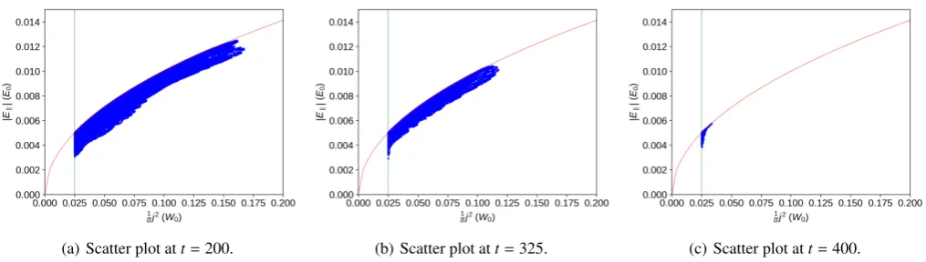
For the results of the present numerical experiment, we have calculatedQin the mid-plane, from the points from which field lines were traced to determineR Ekds. In order to verify the

ac-curacy ofQfor each field line, we have calculated its value by integrating along the field lines starting both from the bottom and from the top boundaries. Any attempt numerically to find the squashing factor in a magnetic field must be done advisedly, in view of several sources of error that arise. The magnetic field on a finite numerical grid is confined by resolution, with an er-ror proportional to the square of the grid spacing. In addition to this, evaluation of the relevant gradients across such a grid by fi-nite differencing introduces an error of second order in step size and consequent dependence on the resolution of the grid. While integration of field lines can be done with high precision, the numerical calculation of Qis limited in accuracy by the error in sub-grid interpolation. Therefore, calculation ofQ, like that ofR Ekds, shows some sensitivity to the scale of the

computa-tional mesh. SinceQhas two values in the mid-plane, one with respect to each boundary, there is an ambiguity in this definition (as noted by Restante 2011; Pariat & Démoulin 2012). The dif-ference made is small, withQsimilar; for consistency, we use the practice of taking the maximum value (e.g. Restante 2011).

As they are calculated from comparable grids, we can di-rectly compare values ofR EkdsandQin various ways.

Con-tours ofQcalculated according to this procedure are depicted in Fig. 4, at selected times so far analysed, namely t = 200,

t = 325, andt =400. Qualitatively, the contour plots in Fig. 1 and Fig. 4 resemble each other in some ways, with highQand largeR Ekdscovering similar areas and showing similar swirling

patterns. However, it is not possible to assess correlation mean-ingfully only through such a visual comparison.

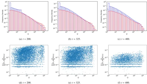
In the top row of Fig. 5, histograms of the values of Q, di-vided according to whether R Ekds = 0 or

R

Ekds , 0, are shown. These clarify the relationship which one may draw be-tween the two: whenR Ekds = 0, indicating the total absence

of reconnection,Qis very likely to be small and deformation of the magnetic field limited. On the other hand,R Ekds,0 shows a greater range in the values ofQ, the distribution more heav-ily focused at values which may indicate the presence of QSLs. Therefore, it appears that the fact of reconnection, but not its rate or extent, may be associated with higherQ.

In the bottom row of Fig. 5, values ofR Ekdsare marked in

scatter plots directly against the corresponding values ofQ. Cor-relation seems weak, as the points are widely dispersed. While there appears to be some correlation, in that largerQis generally associated with higherR Ekds, the effect is less pronounced than

(a)t=175. (b)t=200?.

−1.00 × 10−2

−1.00 × 10−4

−1.00 × 10−6

0.00 1.00 × 10−6

1.00 × 10−4

1.00 × 10−2

E∥  (E0

)

(c)t=225. (d)t=275.

(e)t=325?. (f) t=400?.

Fig. 3.Isosurfaces of localEk. Times shown are (a)t =175, (b)t = 200, (c)t =225, (d)t = 275, (e)t =325, and (f)t = 400. On (a) is

superimposed a sample of field lines in green. The radii of the left, central, and right driving regions are marked on the bottomz=−Lplane. The starred times are subsequently considered in greater detail. The isosurfaces are shaded according to the logarithmic scale on the colour bar.

to indicate the absence of reconnection, but a high value ofQis not necessarily indicative of reconnection.

5.2. Field-line-integrated parallel current

Contours of the electric current, integrated along the same field lines as are used in producing Fig. 1, are shown in Fig. 6. These closely resemble the axial current in the mid-plane plotted in Fig. 5 of Paper I, especially earlier when the current is pre-dominantly field-aligned. Fig. 6 illustrates the progression from the structure associated with the ordered driving motions, to the fragmented final state.

Near the beginning of the experiment, before any instabil-ity, the axial current within each thread is predicted by the lin-earized MHD equations, in particular, Eq. (12). As previously discussed, such linear predictions give a reliable indication of the initial phase of evolution in the system. For this reason, in-tegrating along initially chiefly vertical field lines, the parallel current is most strongly negative on the axis of each thread, van-ishes smoothly atr=a/2, and becomes positive further out. The behaviour is seen in the left-hand thread in the first four, and in

the right-hand thread in the first three, times in Fig. 6. This sim-ple, symmetric appearance disappears following instability and the onset of reconnection, which destroy the original structure of each thread.

The field-line-integrated parallel electric current is also used as a proxy forR Ekdsin the diagnosis and study of magnetic

reconnection (e.g. Wilmot-Smith et al. 2009). Where a uniform resistivity is used, one is a linear scaling of the other, but with a non-uniform, anomalous resistivity, they differ. While the pat-terns and arrangement of parallel current and electric field show clear similarity (cf. Fig. 6 and Fig. 1), the former has a much greater visible structure than the latter, as expected from the crit-ical threshold applied to resistivity in Fig. 1.

(a)t=200. (b)t=325. (c)t=400.

2.0 1.0 × 101

1.0 × 102

1.0 × 103

1.0 × 104

1.0 × 105

1.0 × 106

1.0 × 107

1.0 × 108

≥ 1.0 × 109

Q

Fig. 4.Quasi-squashing factorQfound in the mid-plane, at (a)t=200, (b)t=325, and (c)t=400. We have taken the maximum of the values with respect to the bottom and top planes. The contours are shaded according to the logarithmic scale on the colour bar.

100 ₁₀2 ₁₀4 ₁₀6 ₁₀8

Q

10−12

10−10

10−8

10−6

10−4

10−2

100

Fr

eq

ue

nc

y 

D

en

si

ty

(a)t=200.

100 ₁₀2 ₁₀4 ₁₀6 ₁₀8

Q

10−13

10−11

10−9

10−7

10−5

10−3

10−1

Fr

eq

ue

nc

y 

D

en

si

ty

(b)t=325.

100 ₁₀2 ₁₀4 ₁₀6 ₁₀8

Q

10−12

10−10

10−8

10−6

10−4

10−2

100

Fr

eq

ue

nc

y 

D

en

si

ty

(c)t=400.

(d)t=200. (e)t=325. (f)t=400.

Fig. 5.Histograms of values ofQin the mid-plane, at (a)t=200, (b)t=325, and (c)t=400; and scatter plots showing the distribution of values ofQandR Ekdsat the same point in the mid-plane, at (d)t=200, (e)t=325, and (f)t=400. In order to represent the full distribution on a

single set of axes, the histograms are produced with frequency density (the vertical axis) andQ(the horizontal axis) each on a logarithmic scale. The blue bars indicate the distribution whereR Ekds=0, and the red that where

R

Ekds,0. The histograms are normalized such that the two histograms for each time have a combined area of unity. The scatter plots are also produced on a logarithmic scale.

Examining Fig. 4 and Fig. 6 (specifically, Fig. 6b, 6e, and 6f), we can compare the properties of field-line-integrated paral-lel current and Q. There is a certain degree of similarity in the large-scale structure. Att=200, a thin annulus of higherQ ex-ists around the outer edge of the central thread, where there is also a strong positive current. In the interior, there is some evi-dence of higherQin small patches, particularly on the right-hand side, matching approximately some areas of dominant negative current. Att = 325, the central and right threads have merged into a single entity, with a swirling region of highQseen around

(−0.5,−1.0), where strongly negative current prevails. Similarly, there is a channel of negative current and highQaround x=1 betweeny = −1 andy = 1. The left thread att = 325 shows, inQandR jkds, a behaviour analogous to that seen earlier in

the central thread. By the final time, t = 400, all three of the original threads have merged into a monolithic, disrupted struc-ture, approximately cospatial inQandR jkds. However, within

(a)t=175. (b)t=200. (c)t=225.

­100.0 ­75.0 ­50.0 ­25.0 0.0 25.0 50.0 75.0 100.0

j∥

ds

 (j0 L0

)

(d)t=275. (e)t=325. (f)t=400.

Fig. 6.Contours of the field-line-integrated parallel electric current in the mid-plane. Times shown are (a)t=175, (b)t=200, (c)t=225, (d) t=275, (e)t=325, and (f)t=400, as in Fig. 1 and Fig. 3.

and elevated Qare of similar extent, containing detailed, finer features that are more difficult to correlate.

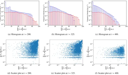
Quantitatively, Fig. 7 shows histograms of the values of R

jkdsfor the two cases where R

Ekdsis zero or non-zero, and

scatter plots ofR Ekdsagainst R

jkds. As is the case forQ, the

histograms reveal that where there is no reconnection, the in-tegrated parallel current is likely to be small, and, for the first two times shown, the highest integrated parallel current values are associated with reconnection. The scatter plots show that if there is reconnection, then a broad range of values of integrated parallel current are possible.

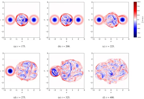
5.3. Locations of Ohmic heating

The Ohmic heating, _σ1j2_{, in the volume is seen in Fig. 8 at three}

of the times shown in Fig. 1, namely, t = 200, t = 325, and

t =400. These again give an illustration of the highly localized nature of the reconnection.

The nature of the anomalous resistivity imposed confines Ohmic heating, as it does reconnection, to sites where j> jcrit.,

since Ohmic heating transfers magnetic energy directly to in-ternal energy as a natural consequence of reconnection. The effects being cospatial and similarly caused, magnetic recon-nection serves to dissipate accumulated magnetic energy, both through conversion to kinetic energy, and through the associated heating.

In the first time shown, in Fig. 8a, it is clear that there is in-tense heating arising in association with the large-scale, helical current sheet that emerges as part of the kink instability. This heating is greatest at the original event that triggers reconnec-tion and excites the MHD avalanche. In the second time shown,

t = 325 in Fig. 8b, a similar process is under way in the third thread, with the most intense concentration in large-scale he-lical features in the left-hand thread. Driving being slower in that thread, less magnetic energy has built up, and the heating is weaker. Nonetheless, it concentrates in a similar crescent-shaped current sheet. At both of these times, there is a multitude of wide-spread, weak, small-scale Ohmic heating events. These mirror the locations of the broad distribution of reconnection sites. By

t = 400, Fig. 8c, only highly fragmented, broadly dispersed Ohmic heating events remain, unsurprisingly as this mirrors the reconnection behaviour.

After the progress of the instability, development of recon-nection, and repeated disruptions via the avalanche process have destroyed the previous order and structure inherent in the driv-ing, Ohmic heating appears in Fig. 8c as highly fragmented, broadly dispersed, and generally weaker. This has been seen in the general heating (Paper I), but most acutely so for Ohmic heat-ing, whose form emphasizes the disordered spread of currents, magnetic reconnection, and heating.

pro-0 20 40 60 80 100

|

|

10−6

10−5

10−4

10−3

10−2

10−1

Fr

eq

ue

nc

y 

D

en

si

ty

 ((

j0

L0

)

−1)

(a) Histogram att=200.

0 20 40 60 80 100

|

|

10−6

10−5

10−4

10−3

10−2

10−1

Fr

eq

ue

nc

y 

D

en

si

ty

 ((

j0

L0

)

−1)

(b) Histogram att=325.

0 20 40 60 80 100

|

|

10−6

10−5

10−4

10−3

10−2

10−1

Fr

eq

ue

nc

y 

D

en

si

ty

 ((

j0

L0

)

−1)

(c) Histogram att=400.

(d) Scatter plot att=200. (e) Scatter plot att=325. (f) Scatter plot att=400.

Fig. 7.Histograms showing the distribution ofR jkdswhere the corresponding field-line-integrated parallel electric field is zero (blue) or non-zero

(red) at (a)t=200, (b)t=325, and (c)t=400; and scatter plots ofR Ekdsagainst

R

jkdsin the mid-plane at (d)t=200, (e)t=325, and (f)

t=400. The histograms are normalized such that the two histograms for each time have a combined area of unity. Both histograms and scatter plots are drawn on logarithmic axes.

(a)t=200. (b)t=325. (c)t=400.

1.00×10−3 1.40×10−2 2.70×10−2 4.00×10−2

Oh

mi

c H

ea

tin

g (

W0t −1)A

Fig. 8.Isosurfaces of Ohmic heating, shaded on a logarithmic scale. Times shown are (a)t=200, (b)t=325, and (c)t=400. The radii of the left, central, and right driving regions are marked on the bottomz=−Lplane.

ceeding from the original kink and initial disruption of each outer thread, followed by a continuing series of lesser events. There is a notable structural similarity between Fig. 8 and Fig. 3, which is expected as Ohmic heating and reconnection occur un-der the identical condition j> jcrit.. However, since Ohmic

heat-ing scales with j2_{, but the parallel electric field withj}

k, the

mag-nitudes of these two properties will vary.

In order to compare further Ohmic heating and reconnection as identified by the contours of the field-line-integrated parallel electric field, displayed in Fig. 1, the field-line-integrated Ohmic heating, similarly determined, is shown in Fig. 9 at the selected times used above. A broad similarity is apparent between these graphs and those at the same times in Fig. 1. In particular, at

t = 200, in Fig. 8a, the Ohmic heating demonstrates a clear concentration and greatest intensity around the location, to the

right of the central thread, where the current sheet associated with the kink instability intersects the mid plane. By the second time,t=325, Fig. 9b very strong heating is evident around the reconnection event sited approximately at (−1.5,−0.9). The in-tegrated electric field and inin-tegrated Ohmic heating have a simi-lar widely dispersed, highly fragmented, and less intense nature at the final time (Fig. 9c). The field-line-integrated electric field and joule heating demonstrate a similarly dispersed, highly frag-mented, and less intense nature at the final time, neither showing any evidence of the thread-like structures seen earlier.

In a scatter plot of Ek

(a)t=200. (b)t=325. (c)t=400.

10−4

10−3

10−2

10−1

100

1 σ2j

ds

 (W

0

L0

)

Fig. 9.Contours of Ohmic heating integrated along field lines traced from the mid-plane, shaded on a logarithmic scale. Times shown are (a) t=200, (b)t=325, and (c)t=400.

(a) Scatter plot att=200. (b) Scatter plot att=325. (c) Scatter plot att=400.

Fig. 10.Scatter plots of

Ek

against Ohmic heating at grid points throughout the domain, at times (a)t=200, (b)t=325, and (c)t=400. The

red line is an upper bound onEkgiven the value of Ohmic heating and assuming current wholly parallel, i.e. √1_σ

q

1

σj2. The green line shows the

minimum possible value of Ohmic heating,η0j2crit..

Since resistivity is locally determined, and integrating along field lines removes spatial information, one may expect the same quantities, when field-line-integrated, to be slightly less corre-lated. However, the evident correlation is, in fact, more pro-nounced. Scatter plots of the field-line-integrated parallel elec-tric field against the field-line-integrated Ohmic heating (Fig. 11) show this correlation, even closer than that of the variables be-fore integration. Except for a few of points (in all cases, fewer than 5% deviate from a best-fitting slope by more than 5%), these integrated terms show almost perfect linearity on the logarithmic scatter plot, which indicates that these parameters scale approx-imately as:

Z

Ekds∝ "Z ₁

σj2ds #α

, (20)

where the value ofαis determined by finding best-fitting slopes between the two quantities. At t = 200, when reconnection is concentrated in a large-scale, helical current structure,α=0.95; however, later, when there are far more small-scale reconnection eventsα=0.99.

The fact that the index is alwaysα≈1.0 is consistent with a material physical determinant of the values of R Ekds and R ₁

σj2dsbeing the length of the field line along which

resistiv-ity is non-zero, which is common between the two. This again

highlights the increasing dominance of the parallel component of current.

5.4. Comparison of indicators: correlation

Because we have the full MHD data and are thus in a position so to do, we use the squashing factorQ, the parallel current, and Ohmic heating, to make inference about the locations of recon-nection. A quantitative comparison can be made with the actual sites of reconnection, identified by a non-zero parallel electric field. A coefficient of correlation is determined betweenR Ekds

andQ,R jkds, and Ohmic heating on the grid in the mid-plane,

and between the local parallel electric field,Ek, and local

instan-taneous Ohmic heating, throughout the entire three-dimensional volume. This quantitative comparison serves as a one-number summary of the scatter plots given in the previous subsections.

(a) Scatter plot att=200. (b) Scatter plot att=325. (c) Scatter plot att=400.

Fig. 11.Scatter plots ofR Ekdsagainst

R ₁

σj2dson field lines traced from grid points in the mid-plane, at times (a)t=200, (b)t=325, and (c) t=400. Superimposed are best-fitting straight lines (red), which have slopes (a) 0.950±0.003, (b) 0.990±0.002, and (c) 0.996±0.005 (95% CIs). Although it appears that there are disproportionately many points beneath the best-fitting line, there is a similar cluster above it; the effect seen here is exaggerated by the logarithmic scaling.

degree to which a monotonic trend exists between two quanti-ties. The comparison is presented in Table 2.

A parallel current may prevail even where there is no recon-nection (i.e. where the critical threshold of the magnitude of cur-rent is not exceeded). For this reason, it is unsurprising that the parallel current, integrated on field lines, is again less strongly correlated with reconnection. In each of the times considered,Q

has a similar level of correlation with reconnection. It appears that this geometric measure of the magnetic field, not account-ing for the resistivity and for the definitive electric field, is less apt to indicate the presence of reconnection, since reconnection does not rely solely upon the magnetic field, but is dependent on, for example, the velocity flows involved.

On the other hand, there is notably a much greater correlation between the field-line-integrated parallel current,R jkds, andQ.

It is clear from Table 1 that there is a lack of evidence for lin-earity between them, yet the presence of a less specific form of positive correlation is apparent in the Kendall coefficient from Table 2. Associated scatter plots, in Fig. 12, emphasize this re-sult.

6. Conclusions

A three-dimensional numerical simulation of an ideal MHD in-stability and the ensuing heating in a multi-threaded coronal loop has been analysed. The onset and spatial location of magnetic reconnection following the commencement of an avalanche pro-cess, triggered by a kink instability, have been determined. Re-connection, initially heavily concentrated in regions prescribed by the driving velocity, adopts, as the instability proceeds and de-stroys the initial structure and order, a highly dispersed and spo-radic distribution of currents and flows. In a three-dimensional field, it is not straightforward to predict the location of reconnec-tion, in contrast with two-dimensional models, in which recon-nection takes place at X-type null points. A localized enhance-ment of the parallel electric field is a defining indicator of a site of magnetic reconnection.

The location of parallel current, which is connected with the defining marker of reconnection, Ek, shows, not unexpectedly,

some correlation with sites of reconnection, as well as having a form, at early times, closely determined by the boundary mo-tions. The Ohmic heating, instigated in common with the oc-currence of reconnection, is similarly distributed, and likewise

evolves from the initial monolithic arrangement to a highly lo-calized one.

This illustrates clearly the necessarily local and confined na-ture of the reconnection. Nonetheless, it is noteworthy that such a chaotic and dispersed distribution of reconnection sites pro-ceeds from the action of a large-scale driver with a very simple spatial structure on an originally uniform magnetic field. Strong evidence emerges of a cascade to smaller scales in the magnetic and electric fields. In this respect, we find agreement with the breadth of evidence that reconnection yields fine-scale structure. The quasi-squashing factor, Q, has been considered as a commonly used predictor for the likely locations of magnetic re-connection. Certainly, Démoulin (2006), for example, observed that evolution under particular forms of shearing can give an ap-proximate relation between maximum current andQ. However, whether there is a quantitative, statistical correlation betweenQ

and the parallel electric field, and whetherQis a good indica-tor in compressible, turbulent fields, have not been tested pre-viously. We find that, although it offers some suggestion of the appearance of reconnection, the two are less thoroughly matched in the situation at hand, of braided magnetic fields with a large guide field component than, for example, in fields produced by submerged sources (e.g. Maclean et al. 2009) or including topo-logical nulls, an especially material distinction in some parts of the corona. In particular, it appears for our case less pertinent for changes in magnetic topology than other measures, such as Ohmic heating, and than past work has documented albeit in very different contexts, as, for instance, De Moortel & Galsgaard (2006a,b) and Galsgaard et al. (2003). The concept ofQappears a good indicator of likely sites of reconnection within fields hav-ing null points, in which topological structures are associated with narrow regions of highQ. Whether these do, in fact, host re-connection is dependent upon the driving velocity field. By lack of null points and a more complex, fragmented distribution of

Q, our model differs from those elsewhere studied. Additionally, our model contains flows driving reconnection that are, largely, self-generated by the evolving field: only during the very early evolution does external driving control reconnection. It remains to be determined in which precise regimes and under which con-ditionsQmay be taken reliably to predict regions of reconnect-ing field lines.

re-Table 1.Correlation of reconnection with potential indicators: Pearson coefficient

Quantities t=200 t=325 t=400

R

Ekds

Q r= +0.222 r= +0.206 r= +0.173 R

Ekds R

jkds r= +0.338 r= +0.313 r= +0.155

R

Ekds

R

jkds

r= +0.332 r= +0.327 r= +0.147

R

Ekds

R ₁

σj2ds r= +0.987 r= +0.997 r= +0.998

Ek

1

σj2 r= +0.965 r= +0.989 r= +1.000

R

jkds

Q r= +0.105 r= +0.103 r= +0.084

Notes.The Pearson correlation coefficient (r) is presented, indicating any linear correlation between field-line-integrated parallel electric field and Q(cf. Fig. 5), field-line-integrated parallel current (cf. Fig. 7), and field-line-integrated Ohmic heating (cf. Fig. 11), found in the mid-plane, and between the parallel electric field and Ohmic heating (cf. Fig. 10), found across the three-dimensional volume. The coefficient is found at the times previously analysed,t=200,t=325, andt=400. Those coefficients shown as 1.000 appear so only through application of the standard rounding conventions for three decimal places.

Table 2.Correlation of reconnection with potential indicators: Kendall rank coefficient

Quantities t=200 t=325 t=400

R

Ekds

Q τ= +0.247 τ= +0.236 τ= +0.164 R

Ekds R

jkds τ= +0.204 τ= +0.193 τ= +0.136

R

Ekds

R

jkds

τ= +0.240 τ= +0.232 τ= +0.144

R

Ekds

R ₁

σj2ds τ= +0.999 τ= +0.999 τ= +0.999

Ek

1

σj2 τ= +1.000 τ= +1.000 τ= +1.000

R

jkds

Q τ= +0.724 τ= +0.655 τ= +0.627

Notes. The Kendall rank correlation coefficient (τ) is presented, indicating any positive correlation between the pairs of indicators, and at the times, considered in Table 1. Those coefficients shown as 1.000 appear so only through application of the standard rounding conventions for three decimal places.

(a) Scatter plot att=200. (b) Scatter plot att=325. (c) Scatter plot att=400.

Fig. 12.Scatter plots ofR jkdsagainstQat (a)t=200, (b)t=325, and (c)t=400. Both the horizontal and vertical axes are logarithmic.

flect the electric field or flows of plasma on which reconnection depends. Converging flows may produce reconnection in even relatively smooth fields; the avalanche model gives a good ex-ample in the fusion of threads. Regions of highQdenote greatly divergent field lines, which may indeed be the hallmark of a cur-rent sheet, but could equally arise from such topological fixtures as null points or separators, which can occur even in a poten-tial field. High Q(indeed, separators with Q → ∞) may arise in potential, current-free fields. Velocity has an important role: current, which facilitates reconnection, has been associated with stagnation flows (Longcope & Strauss 1994). Boundary mo-tions creating such flows have been linked with current sheets at reconnection sites, although the strict need for these motions is queried (Galsgaard et al. 2003; Démoulin 2006). Therefore, high-Qregions are not, by their mere existence, evidence of re-connection, although certainly indicative of the subsequent

pos-sibility: and the two, of course, can be coincident, as is docu-mented.

The Ohmic heating is clearly correlated to a material degree with reconnection. We have sought to determine a quantitative relationship, and, in the field-line-integrated results, have found a fairly consistent power law. Consideration remains to be given to the question of which physical factors influence this index, and whether these may cause it to vary among reconnection regimes.

Acknowledgements. JR acknowledges the support of the Carnegie Trust for the Universities of Scotland. AWH & CEP acknowledge the financial support of

STFC through the Consolidated grant, ST/S000402/1, to the University of St

Andrews. PKB acknowledges financial support of STFC through consolidated

grant ST/P000428/1 at the University of Manchester. The authors are grateful

and Dr Antonia Wilmot-Smith for fruitful discussion and helpful suggestions concerning the manuscript. This work used the DiRAC@Durham facility, man-aged by the Institute for Computational Cosmology, and the Cambridge Service for Data Driven Discovery (CSD3), part of which is operated by the Univer-sity of Cambridge Research Computing, on behalf of the STFC DiRAC HPC Facility (www.dirac.ac.uk). The DiRAC@Durham equipment was funded by

BEIS capital funding via STFC capital grants ST/P002293/1 and ST/R002371/1;

Durham University; STFC operations grant ST/R000832/1; BIS National

E-infrastructure capital grant ST/K00042X/1; STFC capital grant ST/K00087X/1;

and DiRAC Operations grant ST/K003267/1. The DiRAC component of CSD3

was funded by BEIS capital funding via STFC capital grants ST/P002307/1 and

ST/R002452/1 and STFC operations grant ST/R00689X/1. DiRAC is part of the

National e-Infrastructure. This work used the NumPy (Oliphant 2006) and Mat-plotlib (Hunter 2007) Python packages.

References

Arber, T. D., Longbottom, A. W., Gerrard, C. L., & Milne, A. M. 2001, J. Com-put. Phys., 171, 151

Archontis, V. & Hood, A. W. 2013, ApJ, 769, L21

Aulanier, G., Pariat, E., & Démoulin, P. 2005, A&A, 444, 961

Aulanier, G., Pariat, E., Démoulin, P., & DeVore, C. R. 2006, Sol. Phys., 238, 347

Bateman, G. 1978, "MHD Instabilities" (Cambridge, MA: MIT Press) Baumann, G. & Nordlund, . 2012, ApJ, 759, L9

Bingert, S. & Peter, H. 2011, A&A, 530, A112 Bogdan, T. J. & Low, B. C. 1986, ApJ, 306, 271 Boozer, A. H. 2019, Phys. Plasmas, 26, 042104

Browning, P. K., Gerrard, C., Hood, A. W., Kevis, R., & Van der Linden, R. A. M. 2008, A&A, 485, 837

Cairns, R. A. 1985, "Plasma physics" (Glasgow: Blackie)

Carmichael, H. 1964, in "The Physics of Solar Flares", ed. W. M. Hess, National Aeronautics and Space Administration, Science and Technical Information Division, 451–456

De Moortel, I. & Galsgaard, K. 2006a, A&A, 451, 1101 De Moortel, I. & Galsgaard, K. 2006b, A&A, 459, 627 Démoulin, P. 2006, Adv. Space Res., 37, 1269 Démoulin, P. 2007, Adv. Space Res., 39, 1367

Démoulin, P., Bagala, L. G., Mandrini, C. H., Henoux, J. C., & Rovira, M. G. 1997, A&A, 325, 305

Démoulin, P., Henoux, J. C., Priest, E. R., & Mandrini, C. H. 1996a, A&A, 308, 643

Démoulin, P. & Priest, E. R. 1997, Sol. Phys., 175, 123

Démoulin, P., Priest, E. R., & Lonie, D. P. 1996b, J. Geophys. Res., 101, 7631 Dungey, J. W. 1961, Phys. Rev. Lett., 6, 47

Galsgaard, K. & Nordlund, Å. 1996, J. Geophys. Res., 101, 13445 Galsgaard, K., Titov, V. S., & Neukirch, T. 2003, ApJ, 595, 506

Gekelman, W., DeHaas, T., Van Compernolle, B., et al. 2016, Phys. Scr, 91, 054002

Gekelman, W., Lawrence, E., Collette, A., et al. 2010, Phys. Scr, T142, 014032 Gekelman, W., Lawrence, E., & Van Compernolle, B. 2012, ApJ, 753, 131 Haynes, A. L. 2008, PhD thesis, University of St Andrews

Haynes, A. L., Parnell, C. E., Galsgaard, K., & Priest, E. R. 2007, Proc. Roy. Soc. Lond. A, 463

Hesse, M. & Schindler, K. 1988, J. Geophys. Res., 93, 5559 Hones, Jr., E. W. 1979, Space Sci. Rev., 23, 393

Hood, A. W., Browning, P. K., & Van der Linden, R. A. M. 2009, A&A, 506, 913

Hood, A. W., Cargill, P. J., Browning, P. K., & Tam, K. V. 2016, ApJ, 817, 5 Hood, A. W. & Priest, E. R. 1979, Sol. Phys., 64, 303

Hunter, J. D. 2007, Computing in Science & Engineering, 9, 90 Janvier, M. 2017, Journal of Plasma Physics, 83, 535830101 Longcope, D. W. & Strauss, H. R. 1994, ApJ, 437, 851 Low, B. C. 1985, ApJ, 293, 31

Maclean, R. C., Büchner, J., & Priest, E. R. 2009, A&A, 501, 321

Mandrini, C. H., Demoulin, P., Schmieder, B., et al. 2006, Sol. Phys., 238, 293 Masson, S., Pariat, E., Aulanier, G., & Schrijver, C. J. 2009, ApJ, 700, 559 McClements, K. G. 2019, Adv. Space Res., 63, 1443

Milano, L. J., Dmitruk, P., Mandrini, C. H., Gómez, D. O., & Démoulin, P. 1999, ApJ, 521, 889

Neukirch, T. 1995, A&A, 301, 628

Oliphant, T. E. 2006, "A guide to NumPy" (USA: Trelgol Publishing) Pariat, E. & Démoulin, P. 2012, A&A, 541, A78

Parnell, C. E. 2018, in Washington DC American Geophysical Union Geophys-ical Monograph Series, Vol. 235, Electric Currents in Geospace and Beyond, ed. A. Keiling, O. Marghitu, & M. Wheatland, 219–237

Parnell, C. E. & Galsgaard, K. 2004, A&A, 428, 595

Parnell, C. E., Maclean, R. C., & Haynes, A. L. 2010, ApJ, 725, L214

Phan, T. D., Eastwood, J. P., Cassak, P. A., et al. 2016, Geophys. Res. Lett., 43, 6060

Pontin, D. I. 2012, Phil. Trans. Roy. Soc. A, 370, 3169

Priest, E. & Forbes, T. 2000, "Magnetic Reconnection: MHD Theory and Appli-cations" (Cambridge: Cambridge University Press)

Priest, E. R. & Démoulin, P. 1995, J. Geophys. Res., 100, 23443

Raouafi, N. E., Patsourakos, S., Pariat, E., et al. 2016, Space Sci. Rev., 201, 1 Reid, H. A. S., Vilmer, N., Aulanier, G., & Pariat, E. 2012, A&A, 547, A52 Reid, J., Hood, A. W., Parnell, C. E., Browning, P. K., & Cargill, P. J. 2018,

A&A, 615, A84

Restante, A. L. 2011, PhD thesis, University of St Andrews Ross, J. & Latter, H. N. 2018, MNRAS, 477, 3329

Schindler, K., Hesse, M., & Birn, J. 1988, J. Geophys. Res., 93, 5547

Stanier, A., Browning, P., Gordovskyy, M., et al. 2013, Phys. Plasmas, 20, 122302

Sturrock, P. A. 1966, Nature, 211, 695

Tam, K. V., Hood, A. W., Browning, P. K., & Cargill, P. J. 2015, A&A, 580, A122

Tassev, S. & Savcheva, A. 2017, ApJ, 840, 89 Titov, V. S. 2007, ApJ, 660, 863

Titov, V. S., Galsgaard, K., & Neukirch, T. 2003, ApJ, 582, 1172 Titov, V. S., Hornig, G., & Démoulin, P. 2002, J. Geophys. Res., 107, 1164 Vasyliunas, V. M. 1984, in Magnetic Reconnection in Space and Laboratory

Plasmas, ed. E. W. Hones, Jr., 25

Wendel, D. E., Olson, D. K., Hesse, M., Karimabadi, H., & Daughton, W. S. 2013, AGU Fall Meeting Abstracts, SM13A

Williams, B. M. 2018, PhD thesis, University of St Andrews

Wilmot-Smith, A. L., Hornig, G., & Pontin, D. I. 2009, ApJ, 704, 1288 Wilmot-Smith, A. L., Pontin, D. I., & Hornig, G. 2010, A&A, 516, A5 Wright, A. N. 1987, Planet. Space Sci., 35, 813

Wyper, P. F. & Pontin, D. I. 2014, Phys. Plasmas, 21, 102102