Commerce Division
Discussion Paper No. 87
CONTINGENT VALUATION
PAYMENT CARDS:
HOW MANY CELLS?
Dr Geoff Kerr
May 2000
Commerce Division PO Box 84 Lincoln University
CANTERBURY
Telephone No: (64) (3) 325 2811 Fax No: (64) (3) 325 3845 E-mail: [email protected]
Abstract
The dichotomous choice approach to contingent valuation is extremely popular, but obtains
very little information from each respondent and is therefore inefficient. Multiple-bounded
dichotomous choice approaches are more efficient in theory, but theoretical gains are not
always obtained in practice. The multiple-bounded dichotomous choice approach also yields
internally inconsistent responses. Payment cards are another approach to improve contingent
valuation efficiency. At the extremes, dichotomous choice is a two cell payment card, while
open-ended CVM has an infinite number of cells.
This paper reports a split sample test of the impacts on benefit estimates and efficiency
arising from differences in the numbers of divisions on the payment card. Don't know
responses were explicitly included to test for changes in uncertainty because of differences in
cell numbers. Prior expectations were for increased cell numbers to improve efficiency, but
that efficiency gains would eventually be offset by increased frequency of don't know
responses and response variance as cell numbers increased. Contrary to prior expectations,
parameter estimates, standard errors and benefit measures were largely invariant to cell
Acknowledgements
I am grateful to the Lincoln University lecturers who allowed the survey to be administered
in their classes, to the students who completed the survey, and especially to Andrew Cook for
his critical comments and the generous donation of his time to administer the survey. Bert
Contents
List of Tables i
1. Introduction 1
2. Payment Card Design Issues 1
3. Tests for Cell Number Impacts 2
4. Case Study 3
4.1 Method 5
5. Results
7
5.1 Frequency of Don't Know and Non-Useable Responses 8
5.2 Comparison of Common Bid amounts and Bid Distributions 9
5.3 Comparison of Mean and Median Willingness to Pay 9
5.4 Comparison of Response Functions 10
5.5 Likelihood Ratio Test Results 11
6. Discussion and Conclusions 12
List of Tables
1. Bid Divisions on the Three Payment Card Versions 6
2. Summary Survey Response Data 8
3. Chi-Square Test Results for Non-Useable Response Categories 8
4. WTP for Common Bid Amounts 9
5. Maximum Likelihood Model Results 10
6. Likelihood Ratio Test Results 11
7. Estimated Variance-Covariance Matrices 12
1
1. Introduction
Contingent valuation studies may take a variety of formats, including open-ended,
dichotomous choice, multiple-bounded dichotomous choice, iterative bidding, and payment
cards. Recently, the dichotomous choice approach has gained a high level of popularity, but it
comes at the cost of efficiency. Approaches that obtain more information from each
respondent than the single-bounded dichotomous choice approach can be much cheaper to
apply because fewer survey responses are necessary to obtain any pre-determined level of
accuracy. The payment card approach offers one method for increasing efficiency over
dichotomous choice, however it may also introduce a number of biases. For example,
Schuman (1996, p.87) claims “presenting respondents with a set of values to choose from is
now seldom used because of recognition that this kind of framing and anchoring is quite
likely to create bias to and away from certain values”. More specifically, inappropriate choice
of bid range and distribution may introduce information and truncation biases, although
recent research provides mechanisms for circumventing these problems (Rowe et al., 1996).
One potential source of bias is from the number of divisions, or cells, on the payment card. At
the extremes, dichotomous choice represents a two cell payment card, while open-ended
CVM has an infinite number of cells. It is well known that mean WTP from dichotomous
choice CVM generally exceeds that from open-ended approaches (Schulze et al., 1996;
Ready et al., 1996; Bateman et al., 1995; Boyle et al., 1996; Brown et al., 1996). There are
several potential explanations of this discrepancy, including yea saying and anchoring in the
dichotomous choice approach and strategic behaviour in the open-ended approach. Between
the extremes, it is not known what impacts arise from changing the number of divisions on
the payment card. This paper addresses that issue.
2.
Payment Card Design Issues
Increasing the number of divisions for any given range of values narrows down the range
within which each individual’s WTP falls and therefore increases the efficiency of the
payment card approach. However, such increases in efficiency may only be realised if people
have well-formulated and certain preferences. Narrowing the interval size may increase the
2
because values are not sufficiently finely defined. Rowe et al. (1996; p.184) surmise that
“maintaining the range of a payment card and increasing the number of entries to reduce the
interval size may result in a presentation that is unwieldy for respondents and that assumes
more precision than respondents have in the formation of their values.”
The outcome from increasing the number of cells on the payment card may be more item
non-response, biased responses in response to uncertainty, or more “don’t know” responses.
The role of stochastic benefits is emphasised by the high proportions of “don’t know”
responses to single-bounded dichotomous choice approaches, which have provided the
impetus for several investigations of how those responses should be analysed (Ready et al.,
1995; Li and Mattsson, 1995; Wang, 1997).
3.
Tests for Cell Number Impacts
This paper presents an empirical test of survey participants’ responses to payment cards with
different numbers of cells. The presence of stochastic benefits is hypothesised to result in a
positive correlation between the number of “don’t know” responses to the valuation question
and the number of cells on the payment card. The less favourable visual impact of increased
number of cells is hypothesised to increase item non-response as cell numbers increase, it
could also be reflected in an increased presence of “don’t know” responses.
Because there are two hypothesised reasons for an increase in “don’t know” responses with
additional cells, it is not possible to identify the underlying cause of this response behaviour
empirically. One approach to identification of causes of changes in response behaviours is to
interview survey participants to obtain expressions of their cognitive processes whilst
responding to the survey (e.g. “verbal protocol analysis”, Schkade and Payne, 1994). This
paper provides an empirical examination of the existence of differences in don’t know
responses, but does not seek a formal explanation.
In the present study two different items are valued using three payment cards, each with a
different number of cells, but with identical lower and upper bid ranges. Following Rowe et
al. (1996), payment card bids are distributed exponentially. Consequently, range effects are
precluded by the survey design. Centre effects are not expected with this design either
3
The effects of changes in payment card cell numbers are tested in the following ways:
(i) Frequencies of “don’t know” and non-useable responses are compared across
payment card versions.
(ii) Common bid amounts are included on each card to allow for tests of significance of
differences in probability of WTP particular bid amounts, allowing comparison of
different points on distributions.
(iii) Differences in willingness to pay are tested by comparing confidence intervals on
mean and median WTP derived by parameterisation of the response data using
maximum likelihood and bootstrap estimation methods. These “end value” tests have
limited power, as they could show no significant differences in mean and/or median
WTP while there are real differences in underlying responses and WTP distributions
for the different payment cards.
(iv) A chi-square test is used to test for differences between distributions as a whole.
(v) Efficiency changes between versions are evaluated using three goodness of fit
measures.
4. Case
Study
Potential items for valuation were identified in discussions with groups of students at Lincoln
University. Three student facilities were initially identified as being potentially valuable to
students. These were: high quality study space, video tapes of lectures made available in the
University library, and a shuttle bus service between the campus and Christchurch City. The
shuttle bus service was dropped from the survey subsequent to pre-testing that showed that
very few students would actually utilise it. The video and study room facilities were included
in the same questionnaire and were introduced in the following ways.
Videotapes:
4
One approach to dealing with this difficulty would be to place videotapes of all lectures in the library and allow them to be borrowed for free, just like other videotapes in the library collection.
Private study rooms:
Some students find studying difficult in the shared workspaces available for most undergraduates. Issues arise from noise, visual distractions, odours, insecure storage, and limited computer access.
Imagine that a private company has built a set of study rooms adjacent to campus. The rooms all share the following characteristics:
• 2.5 metres x 2.5 metres
• sound proof
• air conditioned/ centrally heated
• whiteboard
• bookshelf
• digital security lock
• 24 hour access
• Pentium III 450mhz computer joined to the Lincoln University network • shared use of a laser printer at 10 cents per page printed
In each case, survey respondents were asked whether they would make use of the facility now
if it were available for free. Only potential facility users then faced the CVM question for that
facility. The payment scenarios were introduced as.
Videotapes:
Now, suppose that the only way to pay for the expense involved in providing this videotape service would be a uniform tuition fee increase for all students.
Imagine there were a binding referendum amongst students to decide whether a
fees-funded videotape programme would be implemented. Over 50% voter support would cause the programme to be put in place.
Please tick the box alongside the highest annual tuition fee increase at which you would vote for the proposal to increase fees to fund videotapes of all lectures.
Private study rooms:
Now, imagine that you had to pay to hire a study room for a full semester.
5
Provision of videotapes is contingent upon a social decision rule, and would provide a
common resource. In contrast, there is no social provision rule for study rooms, they would
be a privately owned facility and only those paying would obtain access. Private ownership
was introduced to minimise protest response from survey participants who thought that the
University should be providing these facilities already. In order to create the strongest
possible incentives to focus on the value of the facility to the student, the provision of rooms is presented as an opportunity that students can choose to ignore.
4.1 Method
Three different payment card formats were applied. Each format had identical lowest and
highest bids ($1 and $300) and allowed “don’t know” and “greater than $300” responses, as
well as zero bids. Application of an exponential function to the range and number of bid
divisions identified bid amounts, which then were rounded in a manner that allowed for as
many common bid amounts as possible between the formats (Rowe et al., 1996). Bid
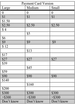
amounts are reported in Table 1. The smallest version of the card contained 9 response
categories (including zero and don’t know), with the intermediate size card having 13
response categories and the large card 18 response categories. Differences in cell numbers are
more significant than indicated by the number of categories because 5 categories are the same
in each case, with zero and $1 anchoring the bottom end of each card and $300, more than
$300, and don’t know anchoring the other end. Efficiency will not be affected by the total
number of cells, but by the number of cells in the region between $1 and $300. These were 5,
9 and 14 for the three versions. The middle response category in each case was $291.
1
6
Table 1
Bid Divisions on the Three Payment Card Versions
Payment Card Version
Large Medium Small
0 0 0
$1 $1 $1
$1.50
$2.50 $2.50 $2.50
$ 4
$5
$6
$9 $9 $9
$ 12
$13
$17
$27 $27 $27
$39
$45 $59
$90 $90 $90
$140
$160 $200
$300 $300 $300
>$300 >$300 >$300
Don’t know Don’t know Don’t know
Shaded cells indicate response categories common to all three versions
Validity of zero bids was tested by a probe question. Answers indicating protest responses
(e.g. university fees are too high already) were deemed to be “invalid zeros”, while those
indicating the facility had no value to them were deemed to be “valid zeros”. Invalid zero
bids were excluded from analysis.
The survey was administered in classes on Lincoln University campus from late May to early
September 1999. Large classes were targeted for administrative convenience. Other selection
criteria included class level, attempts were made to get a range of undergraduate classes from
first year to third year level, and willingness of the lecturer to participate2. The three versions
of the survey were distributed evenly throughout each class. Distribution was made in blocks
of five questionnaires of each version to minimise the chance of neighbours perceiving
differences in questionnaires, but to ensure that seating allocation did not influence the final
2
7
results3. The results are not representative of all students on Lincoln University campus, but
this is irrelevant for the primary purpose of the research, which is to identify impacts of
differences in payment card format.
The survey was given a brief oral introduction concurrent with display of overhead
transparencies that identified the voluntary nature of the survey and guaranteed anonymity.
Students who had completed the survey in other classes were asked not to do it again. The
survey was then distributed, completed and collected. Median completion time was six
minutes. While the survey was being collected participants were told of its hypothetical
nature and its role in research, although the specific purpose was not identified. Participants
were given the opportunity to obtain study results. Because of the context it was not possible
to identify precise response rates, but spot checks indicated these to be in the range of 95% to
100% of those attending the class who had not been surveyed previously.
5. Results
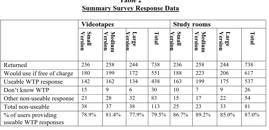
A total of 738 completed surveys was obtained. However, not all of these were useable
because some students who returned surveys would not use the facilities even if they were
provided free of charge. Study rooms would be used by more respondents than video
facilities would be, with 551 respondents (75%) indicating they would use the videotapes if
they were available for free and 617 respondents (84%) stating they would use the study
rooms if they were available for free. Of these respondents, who would theoretically be
willing to pay something for the use of these facilities, 438 (79.5%) provided useable
responses on the payment card for videotape facilities and 537 (87.0%) did likewise for the
study room. Response data are summarised in Table 2.
3
8
Table 2
Summary Survey Response Data
Videotapes Study rooms
Sma
ll
Version Version Medium La
rg e Version To ta l Sma ll
Version Version Medium La
rg
e
Version To
ta
l
Returned 236 258 244 738 236 258 244 738 Would use if free of charge 180 199 172 551 188 223 206 617 Useable WTP response 142 162 134 438 163 199 175 537
Don’t know WTP 15 9 6 30 10 7 9 26
Other non-useable response 23 28 32 83 15 17 22 54
Total non-useable 38 37 38 113 25 23 33 81
% of users providing useable WTP responses
78.9% 81.4% 77.9% 79.5% 86.7% 89.2% 85.0% 87.0%
5.1 Frequency of Don’t Know and Non-Useable Responses
Chi-square tests were undertaken for differences in frequency of “don’t know” responses and
total non-useable responses from the populations of respondents who would use the facilities
if they were available free of charge. Test results are reported in Table 3. There is no
significant difference in don’t know and non-useable response frequencies across the
payment card versions. This result suggests that respondents did not find greater difficulty in
answering when cards had more cells on them. However, it does not mean that the quality of
responses is unchanged between versions.
Table 3
Chi-square Test Results for Non-Useable Response Categories
Facility Comparison Chi-square d.f. Probability
Useable vs non-useable 0.753 2 .686
Video tapes
Don’t know vs others 4.525 2 .104
Useable vs non-useable 2.866 2 .239
Study rooms
9
5.2 Comparison of Common Bid Amounts and Bid Distributions
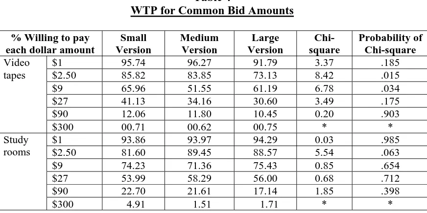
The inclusion of common bid amounts provides the opportunity to apply a chi-square test of
differences in frequency of WTP for those amounts across the different versions. Results are
reported in Table 4. There are only minor differences in rates of WTP between the versions.
There are differences at the $2.50 and $9 bid levels for the videotape facility and at $2.50 for
the study rooms. However, there is no pattern to these differences indicative of any
relationship between the number of cells on the payment card and WTP frequency.
Table 4
WTP for Common Bid Amounts
% Willing to pay each dollar amount
Small Version Medium Version Large Version Chi-square Probability of Chi-square
$1 95.74 96.27 91.79 3.37 .185
$2.50 85.82 83.85 73.13 8.42 .015
$9 65.96 51.55 61.19 6.78 .034
$27 41.13 34.16 30.60 3.49 .175
$90 12.06 11.80 10.45 0.20 .903
Video tapes
$300 00.71 00.62 00.75 * *
$1 93.86 93.97 94.29 0.03 .985
$2.50 81.60 89.45 88.57 5.54 .063
$9 74.23 71.36 75.43 0.85 .654
$27 53.99 58.29 56.00 0.68 .712
$90 22.70 21.61 17.14 1.85 .398
Study rooms
$300 4.91 1.51 1.71 * *
* Numbers of respondents who were WTP this amount were too low for reliable calculation of the chi-squared statistic
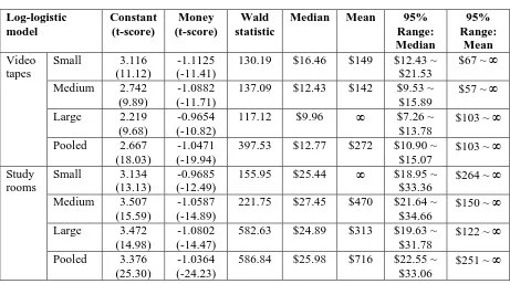
5.3 Comparison of Mean and Median Willingness to Pay
Estimates of mean and median willingness to pay are reported in Table 5. The estimates were
derived using maximum likelihood estimation to fit a log-logistic distribution to the data
(Cameron and Huppert, 1989). The measures of goodness of fit used for dichotomous choice
contingent valuation, such as McFadden’s R2, are not applicable to payment card models
(Kanninen and Khawaja, 1995). Consequently, the Wald test proposed by Harpman and
Welsh (1999) for use with the double-bounded logit model is used. The Wald statistic tests
the improvement of the fitted model over a model that includes only a constant term. The
Wald statistic has a chi-square distribution, with one degree of freedom for all tests in Table
10
Table 5
Maximum Likelihood Model Results
Log-logistic model Constant (t-score) Money (t-score) Wald statistic
Median Mean 95%
Range: Median 95% Range: Mean Small 3.116 (11.12) -1.1125 (-11.41)
130.19 $16.46 $149 $12.43 ~ $21.53
$67 ~ ∞ Medium 2.742
(9.89)
-1.0882 (-11.71)
137.09 $12.43 $142 $9.53 ~ $15.89
$57 ~ ∞ Large 2.219
(9.68)
-0.9654 (-10.82)
117.12 $9.96 ∞ $7.26 ~ $13.78
$103 ~ ∞ Video tapes Pooled 2.667 (18.03) -1.0471 (-19.94)
397.53 $12.77 $272 $10.90 ~ $15.07
$103 ~ ∞ Small 3.134
(13.13)
-0.9685 (-12.49)
155.95 $25.44 ∞ $18.95 ~ $33.36
$264 ~ ∞ Medium 3.507
(15.59)
-1.0587 (-14.89)
221.75 $27.45 $470 $21.64 ~ $34.66
$150 ~ ∞ Large 3.472
(14.98)
-1.0802 (-14.47)
582.63 $24.89 $313 $19.63 ~ $31.78
$122 ~ ∞ Study rooms Pooled 3.376 (25.30) -1.0364 (-24.23)
586.84 $25.98 $716 $22.55 ~ $33.06
$251 ~ ∞
Estimated confidence intervals are the result of 1000 bootstrap replications of the estimation
procedure in each case. They show no significant differences in either mean or median
willingness to pay.
5.4 Comparison of Response Functions
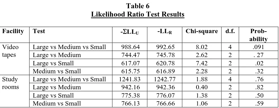
A likelihood ratio test is used to test the hypothesis of equality of the estimated response
functions reported in Table 5 (Welsh and Poe, 1998). The test statistic is approximately
chi-square distributed, with the number of restrictions determining degrees of freedom. The
statistic is:
LR = 2*[ΣLLu– LLR]
where the LLu are the log-likelihood values for independent versions and LLR is the
log-likelihood value for the pooled model which imposes equality of coefficients.
Four tests are possible for each facility, one comparing all three versions with the total pooled
sample and a further three that compare each pair of versions with the appropriate pooled
11
the study room tests. However, the large and small videotape versions showed strong
differences.
Table 6
Likelihood Ratio Test Results
Facility Test -ΣLLU -LLR Chi-square d.f.
Prob-ability
Large vs Medium vs Small 988.64 992.65 8.02 4 .091 Large vs Medium 744.47 745.78 2.62 2 . 27 Large vs Small 617.07 620.78 7.42 2 .02 Video
tapes
Medium vs Small 615.75 616.89 2.28 2 .32 Large vs Medium vs Small 1241.83 1242.77 1.88 4 .76 Large vs Medium 942.16 942.36 0.40 2 .82 Large vs Small 775.38 776.07 1.38 2 .50 Study
rooms
Medium vs Small 766.13 766.66 1.06 2 .59
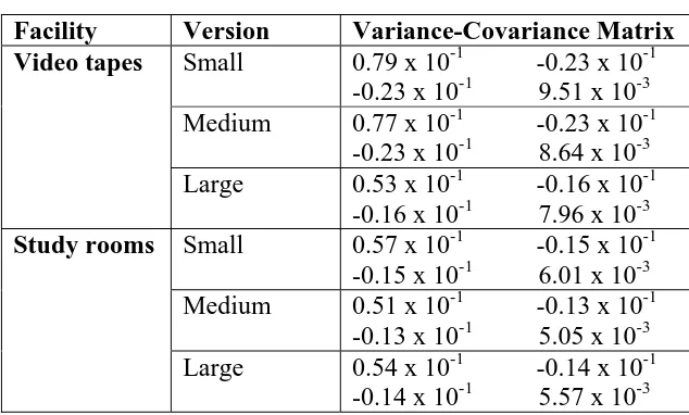
5.5 Comparative Efficiency
Efficiency effects are expected to manifest themselves as small coefficients in the
variance-covariance matrix, larger asymptotic t-scores on estimated coefficients, and narrower bounds
on confidence intervals for estimates of central tendency (Hanemann et al., 1991). The prior
expectation is that efficiency will increase with more divisions on the payment card.
Table 7 reports the estimated variance-covariance matrices for each of the three versions of
the model estimated for each facility. The only differences in variance-covariance matrix
elements are those for the large version of the videotape facility, which are smaller than for
the small and medium versions. However, asymptotic t-scores and 95% confidence interval
estimates for the means and medians are practically invariant to version (Table 5). In these
12
Table 7
Estimated Variance-Covariance Matrices
Facility Version Variance-Covariance Matrix
Small 0.79 x 10⁻¹ -0.23 x 10⁻¹ -0.23 x 10⁻¹ 9.51 x 10⁻³ Medium 0.77 x 10⁻¹ -0.23 x 10⁻¹
-0.23 x 10⁻¹ 8.64 x 10⁻³
Video tapes
Large 0.53 x 10⁻¹ -0.16 x 10⁻¹ -0.16 x 10⁻¹ 7.96 x 10⁻³ Small 0.57 x 10⁻¹ -0.15 x 10⁻¹
-0.15 x 10⁻¹ 6.01 x 10⁻³ Medium 0.51 x 10⁻¹ -0.13 x 10⁻¹
-0.13 x 10⁻¹ 5.05 x 10⁻³
Study rooms
Large 0.54 x 10⁻¹ -0.14 x 10⁻¹ -0.14 x 10⁻¹ 5.57 x 10⁻³
6. Discussion
and
Conclusions
The data obtained here are not representative of all students on the Lincoln University
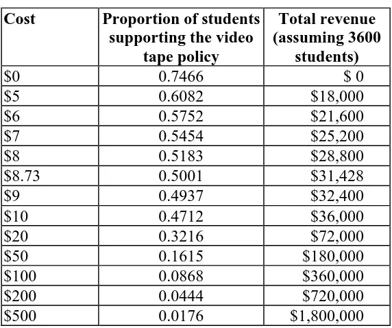
campus, but can provide indicators of value for the facilities examined. Less than 4% of
students would hire study rooms if they were available for $500 per semester. Using a 10%
discount rate, rooms would need to cost less than $10,000 to be viable at this fee level. Table
8 reports the frequency of support for increasing student fees to pay for provision of video
tapes of lectures. Note that these frequencies (and the median) are different from those that
would be derived from the results reported in Table 5 for the pooled model. The difference
arises because Table 8 incorporates those students who have no interest in the facility at all.
Hence, while the estimated median in Table 5 is $12.77, it is derived only for those students
who would, in theory, be willing to pay. The $8.73 median in Table 8 includes all students.
The results of Table 8 indicate that a majority vote would not approve provision of video
tapes if it increased student fees by more than about $8 per year. Consequently, this practice
13
Table 8
Support For and Revenue From Video Tape Policy Cost Proportion of students
supporting the video tape policy
Total revenue (assuming 3600
students)
$0 0.7466 $ 0
$5 0.6082 $18,000
$6 0.5752 $21,600
$7 0.5454 $25,200
$8 0.5183 $28,800
$8.73 0.5001 $31,428
$9 0.4937 $32,400
$10 0.4712 $36,000
$20 0.3216 $72,000
$50 0.1615 $180,000
$100 0.0868 $360,000
$200 0.0444 $720,000
$500 0.0176 $1,800,000
Increasing the number of cells on a payment card is expected to increase efficiency except in
those cases where respondents find it more difficult to answer the contingent valuation
question because of the increased number of payment card cells. This study found no
significant difference on any test for the study room case. Responses were not significantly
different between payment card versions, nor was there any efficiency gain from an increase
in the number of cells. In both cases, frequency of “don’t know” responses was invariant to
number of payment card cells.
The only instance in which a possible small improvement in efficiency was observed was
between the small and large versions in the video tape case, based on the evidence of
coefficient t-scores and variance-covariance matrices. However, higher t-scores and lower
variance in the large payment card case did not translate into narrower confidence intervals
on estimated measures of central tendency. The fitted response distributions for these two
cases also differed significantly. Estimated median willingness to pay declined markedly
between the small and large payment cards for video tapes. While this difference was not
significant at the 95% confidence level applied here, it could be for larger samples. The
direction of change is consistent with observed discrepancies between open-ended and
14
The lack of, or minimal, improvements in efficiency from increasing cell numbers indicates
that respondents did behave differently because of the number of cells on the payment cards.
The uniformity of “don’t know” response rates indicates that differences in responses are
qualitative, not quantitative and are suggestive of an increase in the variance of responses as
cell numbers increase. In the study room case, that behavioural response did not have any
significant effect on estimated bid distributions or measures of central tendency. Bid
distributions did change for the video case, in which event the cards with fewer cells are
likely to be more reliable than cards with more cells. In the absence of evidence that
additional cells provide efficiency benefits, use of small payment cards, which are likely to
place a smaller cognitive burden on respondents and therefore to reduce response variance, is
recommended.
These results are far from conclusive and need to be reinforced with further research. In
particular, it would be instructive to compare results obtained from payment card studies with
those obtained from the dominantly utilised dichotomous choice approach. It would also be
highly desirable to verify the validity of the payment card approach, and variants within that
15
References
Bateman, I. J., Langford, I. H., Turner, R. K., Willis, K. G. & G.D. Garrod (1995) Elicitation and truncation effects in contingent valuation studies. Ecological Economics, 12
pp161-179.
Boyle, K. J., Johnson, F. R., McCollum, D. W., Desvouges, W. H., Dunford, R. W. & S.P. Hudson (1996) Valuing public goods: Discrete versus continuous contingent-valuation responses. Land Economics, 72(3), pp381-396.
Brown, T. C., Champ, P. A., Bishop, R. C. & D.W. McCollum (1996) Which response format reveals the truth about donations to a public good? Land Economics, 72(2), pp152-166.
Cameron, T.A. & Huppert, D.D. (1989) OLS versus ML Estimation of Non-market Resource Values with Payment Card Interval Data. Journal of Environmental Economics and Management, 17, pp230-246.
Hanemann, M.; Loomis, J. & B. Kanninen (1991) Statistical Efficiency of Double-Bounded
Dichotomous Choice Contingent Valuation. American Journal of Agricultural
Economics, 73, pp1255-1263.
Harpman, D.A. & M.P. Welsh (1999) Measuring Goodness of fit for the Double-Bounded Logit Model: Comment. American Journal of Agricultural Economics, 81, pp235-237.
Kanninen, B.J. & M.S. Khawaja (1995) Measuring Goodness of fit for the Double-Bounded Logit Model. American Journal of Agricultural Economics, 77, pp885-890.
Li, C-Z. & L. Mattsson (1995) Discrete Choice under Preference Uncertainty: An Improved Structural Model for Contingent Valuation. Journal of Environmental Economics and Management, 28, pp256-269.
Ready, R.C.; Buzby, J.C. & Hu, D. (1996) Differences Between Continuous and Discrete Contingent Valuation Estimates. Land Economics, 72(3): 397-411.
Ready, R.C.; Whitehead, J.C. & Blomquist, G.C. (1995) Contingent Valuation When
Respondents Are Ambivalent. Journal of Environmental Economics and
Management, 29: 181-196.
Rowe, R.D.; Schulze, W.D. & Breffle, W.S. (1996) A Test for Payment Card Biases. Journal
of Environmental Economics and Management, 31: 178-185.
Schkade, D.A. & Payne, J.W. (1994) How People Respond to contingent Valuation Questions: A Verbal Protocol Analysis of Willingness to Pay for an Environmantal Regulation. Journal of Environmental Economics and Management, 26: 88-109.
Schulze, W., McClelland, G., Waldman, D., & Lazo, J. (1996). Sources of bias in contingent valuation. In D. J. Bjornstad & J. R. Kahn (Eds.), The contingent valuation of
environmental resources: Methodological issues and research needs. Cheltenham,
16
Schuman, H. (1996). The sensitivity of CV outcomes to CV survey methods. In D. J. Bjornstad & J. R. Kahn (Eds.), The contingent valuation of environmental resources: Methodological issues and research needs. Cheltenham, UK: Edward Elgar.
Wang, H. (1997) Treatment of “Don’t Know” Responses in Contingent Valuation Surveys: A
Random Valuation Model. Journal of Environmental Economics and Management,
32: 219-232.
Welsh, M.P. & Poe, G.L. (1998) Elicitation Effects in Contingent Valuation: Comparisons to a Multiple Bounded Discrete Choice Approach. Journal of Environmental Economics