CONSUMPTION FUNCTION – SPECIAL REFERENCE TO QUALITY OF THE COMMODITY CONSUMED

(1)

CONSUMPTION FUNCTION – SPECIAL

REFERENCE TO QUALITY OF THE

COMMODITY CONSUMED

Dr. N. JEYA SEKHAR*

Professor, Department of Mathematics, Sun College of Engineering & Technology,Sun Nagar, Erachakulam, Kanyakumari District, INDIA, Cell. +91 9865389216, E-mail: [email protected]

Dr. D. MATHU

Professor, Department of Mathematics, Sun College of Engineering & Technology, Sun Nagar, Erachakulam, Kanyakumari District, INDIA

Abstract

Use of Traditional Engel analysis in demand functions may not be appropriate if the prices faced by individual consumers are not constants. A procedure to overcome this in this study the work of cox and wohlgenant is extended and used and the results through cox and the bivariate model are compared . The models are applied to house hold expenditures on fish consumed in two different forms

Keywords:Engel analysis, Bivariate normal density model,cox and wohlgenant procedure demand function

1. Introduction

Prais and Houthakker (1955) proposed that prices in cross-sectional data used reflect “quality” effects that should be accounted for prior to estimation. Theil and Houthakker (1952) developed a model to treat the effects of price and quality and used the traditional utility maximization approach to derive the demand functions. In the Houthakker - Theil framework, heterogeneous commodity quantities are defined as the sum of physical quantities of elementary goods in the group and “quality” choice is reflected by a separate set of elements in the household utility function. This model was used and adapted by Deaton( 1987,1988) and Cox and Wohlgenant” But Nelson (1991) pointed out that this model has an in herent ambiquity about how the quantities of composite commodities related to the “Quantity demanded” of consumer demand theory. Supposed the household solves the problem

)

,...,

(

max



x

1

x

k

Subject to

Y

1

=



= k

i i i

x

p

……….………….. (1)

Where

x

i corresponds to the physical quantity of the elementary good

i

, and

p

i is the corresponding

exogeneous price, typically unobservable in the cross-section data,

i

=1,2,…k. Let Y be the consumers income. Now model (1) can be rewritten as

Max U(Q1, …, Qn) Subject to

Y

1

=



= n

G

G G

Q

p

……….. (2)

Where QG is the quantity of composite commodity G, and PG is the corresponding commodity price The demand function is

)

,

(

P

Y

Q

_G

=

_G _G ……… (3) For a composite commodity, can be derived by solving equation (2).

(2)

If it is assumed that the prices of all goods in commodity group G vary proportionally. Nelson called the “base” price of good xi and theil called a quality indicator. From the Hicksian composite commodity

theorem,

From (4) and (5) we have

=



G i

i i G

G

Q

p

x

P

ε

, this links (1) and (2) . As suggested by Nelson, we can define a quantity – weighted sum of elementary goods base prices as a measure of average quality within a group, ie

v

(

/

)

*

(

_G

/

_G

)

G i

i G i

G

=



x

q

p

=

Q

q

∈

where

=



G i

i

G

x

q

ε

and vG is the measure of quantity of composite commodity G. The larger the proportion of higher-priced elementary goods in G, the higher the measure of quality vG

In equation (3), both PG and QG are not observed in typical cross-sectional house hold surveys. However expenditures on commodity G are observed so that



∈

=

G i

i i G i

i

G

P

x

P

x

E

*

= _i _G _G

G i

i

G

P

x

P

Q

P



=

ε

*

When physical quantities (qG) are also observed , a unit value may be calculated as G

G G G G G G

G

E

q

P

Q

q

P

v

V

=

/

=

/

=

……….. (7)

Taking natural logarithm in (7) use get

G G

G

lnP

ln

lnV

=

+

ϑ

………. (8)

The first term in the right-hand side of equation (8) , may be assumed to the constant within group G. The second term is of considerable interest since it is the quality measure for the composite commodity.

Given the relationship (8), we can respecify (3) as

)

,

(

lnV

Y

ω

f

E

_G

=

_G ……….. (9) Where ω represents a vector of household specific characteristics. This specification is adopted since

Q

_G, the “

quantity demanded “ of standard demand theory, is not observed. In empirical applications Deaton (1987) and Cox and wohlgenant used

q

_G, the physical quantity of composite commodity G, instead of

Q

_Gas the measure of demand. The use of

q

_G was interpreted by Nelson as measuring the demand for one particular characteristic of the commodity rather than for the demand of the commodity, itself one reason for using

q

_G may be the interest in obtaining elasticities. However, price elasticities can be obtained from equation (9) ( to be shown).

2. The Empirical Model

An empirical version of (9) for the ith house hold may be expressed as:

i i i

i

lnv

z

E

=

α

₀

+

α

₁

+

α

₂'

+

μ

₁

if

α

₀

+

α

₁

lnv

_i

+

α

₂'

z

_i

>

−

μ

₁_i ………. (10)

0 E

_i

=

otherwise

Here

V

_i is the unit value which is proportional to commodity quality and

Z

_i is a vector of household characteristics, including Y and some variables of ω specified in equation (9).

V

_i cannot be observed for all households. However it may be expressed as

μ

β

i i

i

X

lnV

2 ' 1

0

+

(3)

if

i i i

n

v

z

u

l

1 '

2 1

0

+

α

+

α

>

−

α

Here

X

_i, a subject of W, is a vector of house hold characaterisitcs affecting quality choice. Equation (11) is a empirical version of equation (8)

Here

X

_i is the proxy for

v

_G, which is not observable

0

β

represents

lnP

_G, which may be assumed within the group G.

In this model, it is assumed that

i

1

μ

and

i

2

μ

have a joint normal distribution with mean vector 0 and covariance matrix



_













=

2 2 2 1 2 1 2 1

σ

Let us use













_,

_;

₀

_,

_Σ

20

1

μ

i

N

to denote the bivariate normal density function Wales and Woodland (1980) have suggested several approaches to estimate a system of the form of equations (10) and (11). A likelihood function can be adapted from their results by recognizing that the unconditional probability that household

i

will not consume the commodity is given by

(

0 )

(

,

;

0 ,

)

(

)

2 1 2 ) ( 1 ' 2 1 0 i i i i z lnv i

i

N

d

E

P

i i

θ

μ

α α α α α

−

Φ

=

Σ

=



− + + − ……… (12) In this case

E

_i and

lnV

_i and joint normal variables; hence integration over all values of

lnv

_iyields the marginal density function for

E

_i, which is itself a normal density. The advantage of using

lnV

_i as an argument in the expenditure function avoids the statistical complications associated with

V

_i, since the distribution is truncated at zero.

The likelihood function for a sample of N households, M of which purchase of commodity then is

)

(

)

,

0 ;

,

(

)

,

;

,

(

1 2 1 1 i N M i i i m i

N

lnv

E

L

α

β

Σ

=

Π

μ

Σ

Π

Φ

−

θ

+ =

= ……… (13)

Since the Jacobian of transformation from

to

[

E

lnv

]

i i

,

2 1









_μ

is one. Also, since the expenditure function is linear in

lnv

i, the probability that a household will not purchase the commodity simplifies to an integral over a

univariate normal density function. The probability in equation (12) is expressed as

Φ

(

−

θ

i

)

where

[

]

2 / 1 12 1 2 2 2 1 2 1 ' 2 ' 1 0 1 0

)

2 (

)

(

σ

α

σ

α

σ

α

β

α

θ

+

=

i i

i

z

X

………. (14) And

Φ

is the standard normal distribution function.

The likelihood for the sample may now be written as



+ = = −

₊

_Φ

₋













₋

_Σ

₋

_Σ

=

N m i i M i i i

ln

L

1 1 1 1

)

(

2

1

2

1 log

μ

θ

………. (15)

Where

[

i i i i i

]

i

x

lnv

z

lnv

E

0 1'

' 2 1

0

α

β

α

μ

=

−

The parameters estimated by maximizing equation (15) will be asymptotically unbiased and efficient because all information in the sample is used and the unit value is observed only if the household purchase the commodity is taken into account.

The density function in equation (13) implies that

)

(

)

(

)

0 |

(

E

_i

E

_i ₀ ₁ ₀ ₁'

X

_i ₂'

z

_i

w

₁ _i

E

>

=

α

+

α

β

+

β

+

α

+

λ

θ

………. (16) and

)

(

)

0 |

(4)

( )

θ

i

ϕ

(

θ

i

)

|

(

θ

i

)

λ

=

Φ

and

2 / 1 12 1 2 2 2 1 2 1

1

=

(

σ

+

α

σ

+

2 α

σ

)

w

and

1 12 2 2 1

2

(

)

|

w

=

α

σ

+

σ

From equation (16) the unconditional expectations then are simply

)

(

)

0 |

(

)

(

E

_i

E

_i

E

_i _i

E

=

>

Φ

θ

=

(

)

[

(

)

'

]

₁

(

)

2 '

1 0 1

0 i i i

i

α

β

X

α

z

w

φ

θ

+

Φ

……… (17)

and

)]

(

1 )[

0 |

(

)

(

)

0 |

(

)

(

lnv

i

E

lnV

i

E

i i

E

lnv

i

E

i i

E

=

>

Φ

θ

+

=

−

Φ

θ

=

Φ

(

θ

_i

)(

β

₀

+

β

₁'

X

_i

)

+

w

₂

φ

(

θ

_i

)

+

[

1 −

Φ

(

θ

_i

)](

β

₀

+

β

₁'

X

_i

)

−

w

₂

φ

(

θ

_i

)

=

X

i

' 1

0

β

+

From these expressions, elasticities with respect to each of the expected value can be calculated both expectations for

E

_i, given in equations (16) and (17), are taken as unconditional with respect to unit value. As a consequence, elasticities with respect to

V

_i cannot be obtained. If elasticities conditional on

V

_i are desired, then the probability that

E

_i

=

0

given

lnV

_i must be considered and this probability is given by

Prob.

(

E

_i

=

0 |

lnV

_i

)

=

Φ

(

−

γ

_i

)

………. (18) Where

2 / 1 2 1 2 2 ' 1 0 12

' 2 1

0

(

|

]

/

(

1 )

[

α

σ

β

σ

ρ

γ

i

=

+

lnv

i

+

z

i

+

lnv

i

−

X

i

−

where

2 1 12

/

σ

ρ

=

. The corresponding expectations conditional on

lnv

i are then

)

(

)

1 (

)

,

0 |

(

E

_i

E

_i

lnv

_i ₀ ₁

l

_n

v

_i ₂'

z

_i ₁ 2 1/2 _i

E

>

=

α

+

α

+

α

+

σ

−

ρ

λ

γ

………. (19) and

)

(

)

1 (

)(

(

)

|

(

E

_i

lnv

_i _i ₀ ₁

lnv

_i ₂'

z

_i ₁ 2 1/2 _i

E

=

Φ

γ

α

+

α

+

α

+

σ

−

ρ

π

γ

3. Empirical results with data

In Tamilnadu, Kannyakumari District, which is the southern most part of the state, was scooped out of the then Travancore-Cochin state and now called Kerala, has a different food habit which is not followed any where in Tamilnadu. Fish is a staple food and rarely they consume mutton and Chicken. They use fish is two forms

(i) Curry as a paste material for rice (ii) Roasted form.

To have this food, they, travel even 100 to 150 kms from their place of work to their homes in the night and again go back to work in the early morning every day. Even in Kannyakumari District since the District head quarters is occupied with people from other districts and other states there is a change in the culture, however in the western side of the district the food habit has not changed and hence the western part of this district was chosen as the place for data collection. The researched surveyed 642 individual houses and collected their expenditures over all the food items. This has helped in estimating the unit value of a selected food commodity as the ratio of its associated expenditure to its associated quantity. The survey was conducted over a month. The demographic variables include; all members with age, gender, income, urbanization and the size of the household. The fish is used in two forms; one as curry used for mixing with rice, the other is in the roast form. These two forms are selected separately in the consumption. This separation suggests that unit value may represent an important determinant of household purchases. Maximization of the log likelihood in (15) was done to with the standard computer program. In (15) the first partial derivatives with respect to

α

,

β

,

σ

1

,

σ

2 and

12

σ

were used to calculate the gradient in (15). The Hessian using the derivations the Hessian was computed and it was to found - ive definite.

(5)

Parameter estimates for this bivariate model and the Cox and Wohlgerant model are presented in Table 1 along with three standard errors.

The equation for the logarithm of unit value shows that the logarithm of income is a significant positive factor and the logarithm of family size is a significant negative factor in both procedures. In both procedures, there exists evidence to indicate that gender and employment are no significant factors affecting the unit value. However urbanization and education are key determinates of unit value.

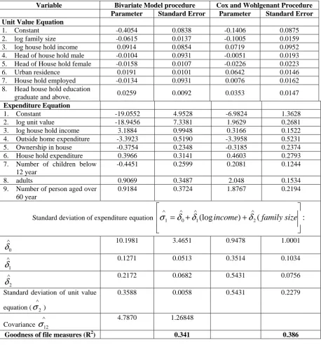
Table 1. Estimated of the Bivariate model and the Cox and Wohlgenant Procedures.

Variable Bivariate Model procedure Cox and Wohlgenant Procedure Parameter Standard Error Parameter Standard Error Unit Value Equation

1. Constant -0.4054 0.0838 -0.1406 0.0875

2. log family size -0.0615 0.0137 -0.1005 0.0159 3. log house hold income 0.0914 0.0854 0.0719 0.0952 4. Head of house hold male -0.0104 0.0931 -0.0051 0.0193 5. Head of House hold female -0.0158 0.0107 -0.0226 0.0223 6. Urban residence 0.0191 0.0101 0.0642 0.0146 7. House hold employed -0.0134 0.0931 0.0076 0.0162 8. Head house hold education

graduate and above. 0.0259 0.0092 0.0353 0.0147

Expenditure Equation

1. Constant -19.0552 4.9528 -6.9824 1.3628

2. log unit value -18.9456 7.3381 1.9629 0.2681 3. log house hold income 3.1884 0.9948 0.3166 0.1522 4. Outside home expenditure -3.3923 0.5190 -3.3958 0.5231 5. Ownership in house -0.3754 0.2348 -0.3185 0.2374 6. House hold expenditure 0.3966 0.3141 0.4603 0.2793 7. Number of children below

12 year

-0.4451 0.2599 0.2081 0.1244

8. adults 0.9069 0.3487 2.048 0.1534

9. Number of person aged over 60 year

0.9184 0.3724 1.8767 0.2194

Standard deviation of expenditure equation ₁ ₀ ₁

(log

)

₂

(

:













+

=

∧ ∧ ∧

∧

size

family

income

δ

σ

∧

0

δ

10.1981 3.4651 0.9478 1.0001

∧

1

δ

0.1271 0.0513 0.3514 0.1034

∧

2

δ

0.2172 0.0682 0.5431 0.0756

Standard deviation of unit value equation (

∧

2

σ

)

0.3588 0.0058 0.5431 0.2279

Covariance ∧

12

σ

4.7870 1.26848

Goodness of file measures (R2) 0.341 0.386

With regard to expenditure equations difference between the two procedure are evident. The logarithm of unit value has negative coefficient in the bivariate model. Hence an inverse relationship between quality and expenditure may be inferred However, the opposite result in found in Cox and Wohlegent approach. Furthermore, since

σ

12is significantly different from zero, the bivariate model reveals that quality and

expenditure are simultaneously determined. In fact, the average correlation implied between the two equations is 0.664. Hence in this case, the Cox and Wohlgenant approach is not an appropriate procedure.

(6)

with the age composition and statistically different from zero, ranging from 0.2081 to 2.048. In the bivariate model, the Coefficients associated with the elderly members are positive and significantly different from zero, but they are 50 percent of those in the other method. Also, in the bivariate model, the Coefficient for adults is not significant.

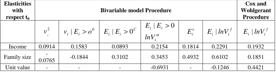
Differences in the two procedures also can be seen from the estimated elasticities. The estimated elasticities are presented in Table 2.

Table 2. Elasticities at Sample means

Elasticities with respect t0

Bivariable model Procedure

Cox and Wohlgerant

Procedure

2

i

v

b

i i

E

o

v

|

>

C

i i

E

|

>

0

_α i

i i

lnV

E

|

>

0

e i

E

f

i i

lnV

E

|

f

i i

lnV

E

|

Income 0.0914 0.1583 0.0893 0.2154 0.1814 0.2291 0.1932 Family size

-0.0765 -0.1844 0.3102 0.3453 0.4932 0.6102 0.1851 Unit value - - - -0.6931 - -0.1246 0.4421

a – unconditional elasticity of unit value

b- Conditional elasticity of unit value conditioned on non zero property of expenditures c- Conditional elasticity of expenditures conditional that expenditure are non zero.

d- Conditional elasticity of expenditures given that logunit values and that expenditures are non zero e – Unconditional elasticity of expenditures.

f- Conditional elasticity of expenditures given the log units values.

The unconditional elasticity of unit value with respect to income is 0.0914, the Coefficient associated with income from table 1. However using equation (16), the elasticity of unit value with respect to income that expenditures are non zero is 0.1583. A negative elasticity of expenditure with respect to unit value was found in the bivariate model (-0.1246), but a positive elasticity of expenditure with respect to unit value was found using Cox and Wohlgenant approach (0.4421).

In both the procedures, age composition of the relationship between price (unit value) elasticity of expenditure,

η

_E

=

∂

lnE

_i

|

∂

lnV

_i, and price elasticity of quantity

η

_q

=

∂

lnq

_i

|

∂

lnv

_i, can be easily derived as

η

q

=

η

E

−

1

because

E

i

=

q

i

V

i. A demand elasticity of -0.1246 was obtained using bivariate model, but

demand elasticity of -0.4325 was obtained using the Cox and Wohlgenant approach. Further both income and family size elasticities are smaller in magnitude in the Cox and Wohlgenant procedure compared to the bivariate model.

Another result found in the bivariate model is that household income has little effect on the two types of fish products expenditures, when not conditioned on unit value. This result is due to the fact that house holds with higher incomes purchase higher quality ( value) foods on the average. Thus, the income effect is effect by the quality(value) effect. The magnitude of the quality (value) effect is captured when conditioning on unit value.

Conclusions:

(7)

References

[1] Cox T.L and M.K. Wohlgenant. “ Prices and Qality Effects in Cross-Sectional Demand Analysis”. Am. J. Agri. Econ 68 (1986): 908-19.

[2] Deaton, A. “Estimation of own and cross-price Elasticities from House hold Survey Data”. J. Econ. 36 (1981):7-30. [3] Deaton,A “Quality, Quantity, and spatial variation of price “Amer. Econ” Rev. 78: 418-30.

[4] Nelson: “Quality variation and Quantity Seggregation in Consumer Demand for food”. Amer. J. Ag. Econ73: 1204-12.

[5] Orme, C. “The small sample performance of the Information Matrix Test”. J. Econ 46:309-32.

[6] Polinsky, A-M. “ The demand for housing : A study in specification and Grouping” Econometricals 447-62. [7] Pr.ais, S.J., and H.J. Houthakker. “The Analysis of family Budgets”. Cambridge univ. Press (1955)