TEXTURE ANALYSIS AND CLUSTERING WITH ELBP-VAR AND
MEAN SHIFT FOR CLASSIFICATION OF HIGH RESOLUTION
IMAGES
Sourabh Singh1, DebasishChakraborty2
1. INTRODUCTION
High spatial resolution imagery facilitates to obtain worthy and comprehensive information about earth‟s surface features together with their geographical relationships. The spatial resolution specifies the pixel size of satellite image covering the earth surface. During recent period, more and higher resolution satellite images namely CARTOSAT-2 1m and IKONOS 1m are available for earth observations. The spectral or pixel-based classification technique consists of K-Means [11], Fuzzy C Means [1] and methods of Minimum Distance [18], which considers only the spectral pattern to segment the image. These techniques are not sufficient to classify high-resolution satellite images due to variability of spectral and structural information in such images [5, 6]. The spatial pattern or texture analysis becomes necessary to classify high-resolution images. Thus the number of texture-based classification technique namely GLCM (Gray Level Co-occurrence Matrix) [20], Markov random field (MRF) model [10], Gray scale rotation invariant [13], Hölder exponents [4] have been developed for classifying high spatial resolution images. Majority of the texture-based classification techniques measure the spatial structure of local image texture, but discards contrast which is another important property of local image texture. Therefore these texture based classification algorithm does not yield desired results [7].
Some more techniques namely watershed approach [17], region-growing approach [6,2], region merging approach etc. are in use for clustering high spatial resolution remote sensing images. Application of these approaches for classification of images either leads to under-segmentation or over-segmentation [8]. Structural image indexing approach [21], semi-supervised feature learning approach and multi-scale manner using SVM approach [12] are also used and found quite useful in classifying high spatial resolution remote sensing images.
In last few years the mean-shift [19, 14, and 3] and LBP [9, 15] has been used individually for clustering high-resolution images. But most of them have been developed for extracting specific features from high resolution images. Hence the present study is carried out with a specific objective of developing a clustering algorithm for capturing all type of features in high spatial resolution images using ELBP-VAR and Mean-Shift based technique together. The ELBP (Enhanced Local Binary Pattern) operator together with VAR (variance) is used for measuring texture while Mean-Shift is used for clustering texture transformed image. The proposed approach is implemented on high resolution IKONOS PAN image having spatial resolution 1 m.
2. METHODOLOGY
The proposed approach for clustering high spatial resolution image P has two main steps: (i) image transformation, and (ii) clustering the texture transformed image. In the first step each pixel of the image P is transformed into degree of texture on the basis of its neighbor, while the transformed image is clustered in the second step.
1
Department of Computer Science and Engineering, SMIT, Majitar, Rangpo, Sikkim, India 2
Regional Remote Sensing Centre-East, National Remote Sensing Centre, ISRO, New Town, Kolkata, West Bengal, India Abstract- In this study, an enhanced local binary pattern (ELBP) operator is evolved for quantifying spatial structure. Variance (VAR) is used for measuring contrast around the pixel of the image. Thereafter, the quantified ELBP and VAR value are used together to transform the image for measuring the texture. The Mean-Shift based two-step iterative procedure for clustering the transformed image is adapted to (i) identify the range of texture that is densely occupied in the kernel (ii) partition the textures into a cluster that matches with the range. Subsequently similar type of clusters are grouped together to get classified image. Texture values [noise or not associated with the other cluster] are clubbed to a nearest possible clust er using the contextual clustering. IKONOS 1m PAN images are classified using the proposed clustering algorithm and found that the classification accuracy is more than 89%.
Key Words -High resolution image; clustering; Mean Shift; IKONOS; LBP; classification.
2.1 Image Transformation
TheEnhancedLocal Binary Pattern (ELBP) Operator and VAR are used together to transform the image for measuring the texture. The ELBP operator measures the spatial structure around each pixel of P. Besides spatial structure, contrast of the local image holds important property for measuring the texture around the pixel. Therefore VAR is used for measuring the contrast around the pixel.
2.1.1 EnhancedLocal Binary Pattern (ELBP) operator for measuring spatial structure around each pixel of the image
The Local Binary Pattern (LBP) Operator is based on a binary code describing the local spatial structure [16, 6]. This code is built by thresholding a local neighborhood by the grey value of its center. The eight neighbors are labeled using a binary code {0, 1} obtained by comparing their values to the central pixel value. If the tested grey value is below the grey value of the central pixel, then it is labeled 0, otherwise it is assigned the value 1. The obtained value is then multiplied by the weights given to the corresponding pixels. The weight is given by the value 2i+1. Summing the obtained values gives the measure of the LBP Operator. Advantages of using LBP Operator in high spatial resolution images are that (i) it can be used as a tool to measure the spatial structure around each pixel of the image and (ii) it does not require any prior information about the pixel intensity, (iii) theoretically and computationally LBP Operator is simple.
In this study, a new LBP operator is evolved to measure the spatial structure around each pixel of P. This new LBP operator builds the binary code of the local neighborhood considering a threshold „t‟. Let gδ is the grey value of the center pixel‟s (i.e. (x,y) pixel‟s). Then intensity values of its neighborhood pixels in the range gδ ± t are labeled as 0 and intensity values of the pixels either below or above this range are labeled as 1. Here, „t‟ is computed using equation 1.
t (1)
Where, and denote maximum and minimum intensity value around P(x,y) respectively and N denote number of pixels around P(x,y). The advantage of using threshold „t‟ is that the noise tolerance interval in new LBP is [gδ – t; gδ + t], where t is not constant rather it changes with the variation of the gray levels of the neighborhood. Thus we can infer that proposed LBP codes are more resistant to noise. Moreover the new LBP operator uses a series of circles (2D) centered on the pixel with incremental radius values for measuring the spatial structure. The significance of using series of circles is that (i) the circular neighborhoods enable a definition of a rotation invariant texture and (ii) multiple circles facilitate to describe large neighborhoods with a relatively short feature vector than a circle to compute the spatial structure around the pixel. It measures rotation invariant texture for each circularly symmetric neighborhood and finally adds all measure to get th e spatial structure around the pixel. The proposed LBP operator is named as Enhanced Local Binary Pattern Operator (ELBP) operator. The spatial structure around each pixel of P is computed using ELBP operator and is given as follows:
Number of 1 to 0 or 0 to 1 transition ξ1 for the circle of radius r =1 is computed by using the equation 2.
- (2)
where, uis the intersected pixels on the perimeter of the circle of radius r =1, gδ is the grey values of the center pixel of the circle of radius r =1 and
Similarly 1 to 0 or 0 to 1 transition ξ3 and ξ5 for the circle of radius r =3 and r =5 are computed respectively. Finally the total transition ξC is obtained by using equation 3.
(3) The ξC is considered here as the ELBP value of (x,y) pixel i.e. ELBP (x,y) = ξC. Thus for each pixel (x,y) of the original image P a ELBP value ξC is obtained.
2.1.2 VAR for measuring contrast around each pixel of the image
The VAR (σ2) of the neighbor of each pixel (x,y) over the whole image is computed to obtain the contrast or σ2 value of (x,y). To achieve this initially for each pixel (x,y), a series of grey values { g0, g1, …., gu-1, h0, h1, …., hu-1 , i0, i1, …., iu-1 } as described earlier are acquired. Then the σ2 (x,y) is obtained by using the equation 4.
/ N (4) Where,
{ a1, a2, ….,aN } = { g0, g1, …., gu-1, h0, h1, …., hu-1 , i0, i1, …., iu-1 }, N = 3u and
Thus ELBP (x,y) and σ2 (x,y) for each (x,y) of the original image P are obtained. Subsequently, these values are used in the equation 5 to get the corresponding pixel value (x,y) in the transformed the image T. Each pixel (x,y) of T represents the degree of texture around that pixel.
(5)
2.2Clustering transformed image
In this section transformed image T is clustered. An iterative clustering procedure is adapted to: (i) identify densely populated range within the window, (ii) identify the cluster contained in the window.
2.2.1 Identification of densely populated range within the kernel
In this section densely populated range contained in the kernel is computed using the Mean-Shift technique (Chakraborty et al. 2008; Comaniciu et al. 2002) for using it as criteria for clustering the pixels. The advantage of using Mean Shift based clustering is that it does not require prior knowledge of the number of clusters. The number of clusters is obtained automatically by finding the centers of the densest region of the data set. Moreover this technique is not application dependent (Chakraborty 2012).
It is a three steps iterative technique that points towards the direction of the densest region of a data set. Preliminarily mean texture value (Gmean) is computed.In the second step select those pixels in G whose texture difference from Gmean is less than €. This step is represented by equation (6).
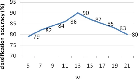
(6) Where, G is a two dimensional window of size w2, G [i,j] represents the texture value of the pixel in [i,j] position of G and € is a threshold. Here, „w‟ is user defined value. To find optimum w, IKONOS PAN image (Figure III(a)) having resolution of 1m x 1m of size 256 x 256 pixels is used. Further, the proposed clustering approach is implemented on this image for different „w‟ values.
The mean texture value (Gmean) of selected pixels is again calculated in third step. Iterates the second and third steps till it converges or reaches a fixed number of iteration. During each iteration € is decreased by a small value
. The convergence isreached only while |Gmean-Gmean|< €, where, Gmean and Gmean are mean texture values of selected pixels respectively after subsequent iteration. If this does not happen within a certain number of iterations then iteration is stopped. Once the convergence is reached or iteration procedure is stopped gets a set ξ s.t ξ G. The set ξ contain only that range of pixels that are densely populated within G. Thus gets the densely populated range DR within G such that ξ min < DR < ξ max, where ξ min = Minimum (ξ), ξ max = Maximum (ξ). The range DR becomes the criteria for clustering pixels.
2.2.2 Identification of the cluster contained in the kernel
Cluster is the pixels within the window whose textures values belong to DR. Pixels belonging to the cluster are significantly correlated. The texture values in the transformed image not included in DR is considered as background. Such texture values, either belongs to another cluster or do not belong to any cluster (noise; are not significantly associated with other texture values). Texture values belonging to other clusters are not considered at the time of range calculation for the current cluster. Thereafter similar clusters are grouped together to get the classified image. The classified image obtained by the presented clustering algorithm consists of noise. A pixel in the classified image is considered as noise if its neighbors are not having similar class value as that pixel. The contextual information is used to cluster those noises. It is a two-step procedure. In the first step it computes the weight of each class residing in the neighborhoods, while the maximum weighted class is identified in the second step. The noise value is clubbed to the class which has the maximum weight in that neighborhood. A h x h size of kernel is considered to use the contextual information.
(i) Cluster weight is computed using equation 7
Wt_Clusterl (7)
Where, l is the number of class residing in the kernel, Freql is the total number of pixel falling in lth class residing in the kernel and Wt_Clusterl is the possibility (or weighting factor) to assign the pixel value in the lth class.
(ii) Maximum weighted class is identified using equation 8
Max_WT_Cluster = [sup {Wt_Clusterl }, k=1 to Q, ] (8) Where, Q is the number of class contained in the kernel
3. RESULTANDDISCUSSION
In the present study, the proposed classification algorithm is implemented on IKONOS PAN data having spatial resolution of 1m adapting different „w‟ values of 5,7,9,11,13,15,17,19,21 respectively. The average classification accuracy is assessed for different „w‟ values using the ground truth data. Figure 2 shows the classification accuracy with different „w‟. From figure 2, we can conclude that „w‟ affects the success rate in classifying IKONOS PAN images substantially. Therefore, a suitable selection of „w‟ or kernel size is important for measuring texture. It is worth noticing that the optimal „w‟ is dependent on the image resolution. In this study, with the resolution of 1m, w = 13 achieves the best performance in IKONOS PAN image classification.
Figure 2: Classification accuracy as a function of w
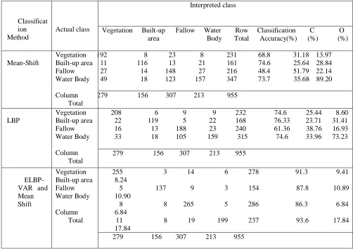
The “Mean-Shift” based method (Cheng et al 2013) ,“LBP” based method (Su et al 2015) and Proposed “ELBP-VAR and Mean-Shift” based clustering method have been applied on two different 1 m PAN (IKONOS) images (size 256x256 pixels) of (i) vegetation, (ii) built-up area, (iii) water bodies, and (iv) fallow (shown in Figure III (a) and III (e)). Texture is visible in both the images. The results of proposed method are then compared with the results obtained from the analysis based on “Mean-Shift” and “LBP” respectively.
for each approach is shown through confusion matrix. The confusion matrices (Table 1) calculated for IKONOS classified images (Figure III (b), III (c) and III (d)) showed that the accuracy of classifying vegetation, built-up area, fallow and Water bodies are (69%, 75%, 48% and 74% respectively) by “Mean-Shift” based method and (75%, 76%, 61% and 75% respectively) by “LBP” based method whereas (91%, 88%, 86% and 94% respectively ) by the “Proposed clustering” method.
The clustered output with respect to the two input images (Figure III (a) and III (e)) shows that the “Mean-Shift” based method under segment (i) fallow and vegetation mixed with water bodies shown in Figure III (b) and III (f), (ii) built-up area mixed with fallow and vegetation shown in Figure III (f), (iii) fallow mixed with built-up area shown in figure III (f). This discrepancy decreases the classification accuracy of vegetation, fallow, water bodies and built-up area as shown in Table 1. The “LBP” based approach overcomes these discrepancies in some extent. It is found that the superposition of fallow, water body, vegetation area becomes less as shown in figure III (c) and III (g). Moreover decreased discrepancies increase the accuracy in classifying fallow, water body and vegetation areas (shown in Table 1). But the Proposed clustering method mostly overcomes these discrepancies as shown in figure III (d) and III (h). Thus the improvement in classification accuracy is found in Table 1.
The method is also applied on other two different 1 m PAN (IKONOS) images: (i) figure IV(a) of fallow, vegetation, built-up area and water bodies and (iii) figure IV (c) of bare soil, vegetation, fallow and built-up area. The output results (figure IV (b) and IV (d)) shows that the method satisfactorily discriminate vegetation, fallow, built-up area, bare soil and water bodies.
Classificat ion Method Actual class Interpreted class
Vegetation Built-up Fallow Water Row Classification C O area Body Total Accuracy(%) (%) (%)
Mean-Shift Vegetation Built-up area Fallow Water Body Column Total
192 8 23 8 231 68.8 31.18 13.97 11 116 13 21 161 74.6 25.64 28.84 27 14 148 27 216 48.4 51.79 22.14 49 18 123 157 347 73.7 35.68 89.20
279 156 307 213 955
LBP Vegetation Built-up area Fallow Water Body Column Total
208 6 9 9 232 74.6 25.44 8.60 22 119 5 22 168 76.33 23.71 31.41 16 13 188 23 240 61.36 38.76 16.93 33 18 105 159 315 74.6 33.96 73.23
279 156 307 213 955
ELBP-VAR and Mean Shift Vegetation Built-up area Fallow Water Body Column Total
255 3 14 6 278 91.3 9.41 8.24
5 137 9 3 154 87.8 10.89 10.90
8 8 265 5 286 86.3 6.84 6.84
11 8 19 199 237 93.6 17.84 17.84
279 156 307 213 955
C: Commission error, O: Omission error
Figure III (a) Figure III (e)
Figure III (b) Figure III (f)
Figure III(c) Figure III (g)
Figure III (d)
Figure III (h)
Scale (meters):
0 50
Figure III (d)
Vegetation
Built-up area
Water Bodies
Figure III a-h: (a) IKONOS image showing vegetation, built-up area, fallow and water bodies categories, (b) Classified image obtained by applying “Mean-Shift” based method on figure (a), (c) Classified image obtained by applying “LBP” based method on figure (a), (d) Classified image obtained by applying proposed “ELBP-VAR and Mean-Shift” based clustering method on figure (a), (e) IKONOS image showing built-up area, fallow, water bodies and vegetation categories, (f) Classified image obtained by applying “Mean-Shift” based method on figure (e), (g) Classified image obtained by applying “LBP” based method on figure (e), (h) Classified image obtained by applying proposed “ELBP -VAR and Mean-Shift” based clustering method on figure (e).
Figure IVa-d: (a) IKONOS image showing fallow, built-up area, vegetation and bare soil categories, (b) Classified image obtained by applying “ELBP -VAR and Mean-Shift” on figure (a), (c): IKONOS image showing vegetation, fallow, built-up area and water bodies categories, (d): Classified image obtained by applying “ELBP -VAR and Mean-Shift” on figure (c)
4. CONCLUSION
In the present study, ELBP operator is evaluated to compute the spatial structure and VAR is used for measuring contrast around each pixel in the image. Subsequently ELBP and VAR value of each pixel in the image is used together to transform the image for measuring the texture. The mean-shift based clustering technique is used to classify the texture transformed image. From the results of the experiments, it is found that the proposed method is useful to classify high spatial resolution images. Moreover, it can be considered as an intuitively appealing and unsupervised classification algorithm. As a result the method is potentially useful to classify high spatial resolution panchromatic images more efficiently.
5. ACKNOWLEDGEMENT
Authors are thankful to the Director, NRSC, Hyderabad, India and CGM, RCs, NRSC, Hyderabad, India for their guidance and support on carrying out this research. Authors are also grateful to the GM, RRSC-East, NRSC, Kolkata, India for his encouragement during the course of this study
6.REFERENCES
[1] [1] J. C Bezdek, R. Ehrlich and W Full, “FCM: the Fuzzy c-Means clustering algorithm”, Computers and Geosciences,vol. 10, pp.191-203, 1984. [2] [2] A.P Carleer, O. Debeir, E. Wolff, “Assessment of Very High Spatial Resolution Satellite Image Segmentations”, Photogrammetric Engineering &
Remote Sensing, vol. 71(11). pp. 1285–1294, 2005
[3] [3] D. Chakraborty, G K Sen, S Hazra and A Jeyaram, “Clustering for High resolution monochrome satellite image segmentation”. International Journal of Geoinformatics. Vol.4(1), pp. 1-9, 2008.
Figure IV (a)
Figure IV (c)
Scale (meters): 0 50
Figure IV (a)
Figure IV (b)
[4] [4] D. Chakraborty, G.K Sen, S Hazra, “High-resolution satellite image segmentation using H¨older exponents”, J. Earth Syst. Sci., vol.118(5),pp. 609-617, 2009.
[5] [5] D. Chakraborty, G K Sen, S. Hazra, “Image segmentation Techniques”, LAP LAMBERT Academic Publishing, Germany, pp. 1 -128, 2012. [6] [6] D. Chakraborty, “Development of mathematical methods on spatio-spectral clustering of high-resolution images”, Phd dissertation. Jadavapur
University,India, 2012.
[7] [7] D. Chakraborty, S. Singh, D. Dutta, “Segmentation and classification of high spatial resolution images based on Hölder exponents and variance”, Geospatial Information Science, vol. 20(1), pp. 39-45, 2017.
[8] [8] B. Chen, F. Qiu, B. Wu and H. Du, “Image Segmentation Based on Constrained Spectral Variance Difference and Edge Penalty”, Remote Sensing, vol. 7, pp. 5980-6004, 2015.
[9] [9] J.Cheng, L. Li, B. Luo, S. Wang and H. Liu, “High-resolution remote sensing image segmentation based on improved RIU-LBP and SRM”, EURASIP Journal on Wireless Communications and Networking, 2013,.
[10] [10] D A Clausi, B Yue, “Texture Segmentation Comparison Using Grey Level Co-occurrence Probabilities and Markov Random Fields”, Proceedings of the 17th International Conference on Pattern Recognition (ICPR‟04), (Available at: http://ieeexplore.ieee.org/stamp/), 2004.
[11] [11 J A ] Hartigan and M A Wong, “A K-means clustering algorithm”, Appl. Stat., vol. 28(1), pp.100–108, 1979.
[12] [12] X. Huang, L. Zhang, “An SVM ensemble approach combining spectral, structural, and semantic features for the classification of high-resolution remotely sensed imagery”, IEEE Transactions on Geoscience and Remote sensing, vol. 51(1), pp. 257-272, 2013.
[13] [13] V V Klemas, “Remote Sensing of Coastal Resources and Environment”, Environmental Research, Engineering and Management, vol. 2(48), pp.11-18, 2009.
[14] [14] H. Lu, C. Liu, Nai-wen Li, Jia-wei Guuo, “Segmentation of high spatial resolution remote sensing images of mountainous areas based on the improved mean shift algorithm”, Journal of Mountain Science, vol. 12(3), pp. 671-678, 2015.
[15] [15] B. Luo, J. Cheng, “Segmentation algorithm of high resolution remote sensing images based on LBP and statistical region merging”, International Conference on Audio, Language and Image Processing (ICALIP), 2012.
[16] [16] A. Lucieer, A. Stein, P. Fisher, “Texture-based segmentation of high-resolution remotely sensed imagery for identification of fuzzy objects”, International Journal of Remote Sensing, vol. 26(14), pp. 2917-2936, 2005.
[17] [17] B.Mathivanan, S. Selvarajan, High spatial resolution remote sensing image segmentation using marker based watershed algorithm. J. Acad. Indus. Res., vol. 1(5), pp. 257-260, 2012.
[18] [18] J A Richards, “Remote Sensing Digital Image Analysis: An Introduction”, Springer-Verlag, pp. 265-290, 1995 .
[19] [19] T. Su, H. Li, S. Zhang, and Y. Li , “Image segmentation using mean shift for extracting croplands from high-resolution remote sensing imagery”, Remote Sensing Letters, vol. 6(12), pp. 952-961, 2015.
[20] [20] F. Tsai, M J Chou, “Texture Augmented Analysis of High Resolution Satellite Imagery In Detecting Invasive Plant Species”, Journal of the Chinese Institute of Engineers, vol. 29(4), pp. 581-592, 2006.
[21] [21] G, S. Xia, W. Yang, J. Delon, Y. Gousseau, H. Sun, H. Maître, “Structural high-resolution satellite image indexing”, ISPRS TC VII Symposium-100 Years ISPRS, vol. 38, pp. 298-303, 2010.
[22] [22] W. Yang, X. Yin, G. S Xia, “Learning high-level features for satellite image classification with limited labeled samples”, IEEE Transactions on Geoscience and Remote Sensing, vo.53(8), pp.4472-4482, 2015.