Predicting Cache Contention with Setvectors
Michael Zwick, Florian Obermeier and Klaus Diepold
∗Abstract—In this paper, we present a new method called setvectors to predict cache contention intro-duced by co-scheduled applications on a multicore processor system. Additionally, we propose a new metric to compare cache contention prediction meth-ods. Applying this metric, we demonstrate that our setvector method predicts cache contention with about the same accuracy as the most accurate state-of-the-art method. However, our method executes nearly 4000 times as fast.
Keywords: Setvectors, Coscheduling, Cache con-tention.
1
Introduction
With multicore processors, chip manufacturers try to sat-isfy the ever increasing demand for computational power by parallelization on thread or process basis, making per-formance of computer systems more and more indepen-dent from the saturated processor clock speed. However, one important limitation that does not rely on proces-sor clock speed, but on the computational power of the processor, is the ever increasing processor memory gap: Although both, processor and DRAM performance, grow exponentially over time, the performance difference be-tween processor and DRAM grows exponentially, too. This happens due to the fact that“the exponent for pro-cessors is substantially larger than that for DRAMs” [7] and “the difference between diverging exponentials also grows exponentially” [7].
A way to deal with the exponentially diverging mem-ory gap is to transform computational performance into memory hierarchy performance, making memory perfor-mance not only benefit from improvements of the mem-ory hierarchy system, but also from better (and in a much higher rate evolving) processor technology. One possibil-ity therefore is to spend computational power to find good application co-schedules that minimize overall cache con-tention. Reducing DRAM accesses by optimizing cache performance is a key issue in todays and tomorrows com-puter architectures.
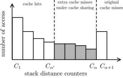
L2 cache performance has been identified as a most cru-cial factor regarding overall performance degradation in multicore processors [2]. Figure 1 shows the effect of L2 cache contention on the SPEC2006 benchmarkmilc,
run-∗Lehrstuhl f¨ur Datenverarbeitung, Technische Universit¨at M¨unchen, 80333 M¨unchen, Germany
0 50 100 150 200 250
0.2 0.4 0.6 0.8
chunks (1 chunk = 2 instructions)20
L2 cac
he hitrate (%)
[image:1.595.308.531.199.381.2]milc @c0: milc milc @ c0: milc, c1: astar milc @ c0: milc, c1: gcc milc @ c0: milc, c1: bzip2 milc @ c0: milc, c1: gobmk milc @ c0: milc, c1: lbm
Figure 1: L2 cache hitrate degradation for the milc SPEC2006 benchmark when co-scheduled with different applications.
nig on core c0 of a dual core processor, when co-scheduled with applicationsastar,gcc,bzip2,gobmk andlbmon core c1. It can easily be seen that the performance of milc heavily degrades when co-scheduled with thelbm bench-mark; other co-schedules however, have a much lower per-formance burden.
A requirement in order to optimize co-schedules for cache contention is a good metric to predict cache contention of application co-schedules from specific application charac-teristics. Although a number of methods have been in-vestigated that predict L2 cache performance from some application characteristics for single core processors, so far only little effort has been spent to predict L2 cache performance of co-scheduled applications in a multicore scenario.
The remainder of this paper is organized as follows: Section 2 presents state-of-the-art techniques to pre-dict cache contention; section 3 introduces oursetvector method. In section 4, we propose a new metric called MRD (mean ranking difference) to compare cache con-tention prediction techniques and discuss the parameters applied to our simulation. In section 5, we present our results. Section 6 concludes this paper.
2
State-of-the-art
Cache
Contention
Prediction Techniques
In this section, we describe state-of-the-art techniques to predict cache contention in multiprocessor systems, namly Alex Settle et al.’sactivity vectors [6] and Dhruba Chandra et al.’s stack distance based FOA (frequency of access) andSDC (stack distance competition) model [1] and their circular sequence based Prob (probability) model [1].
2.1
Settle et al.’s Activity Vectors
Alex Settle et al. studied processor cache activity and ob-served that “program behavior changes not only tempo-rally, but also spatially with some regions hosting the ma-jority of the overall cache activity.”[6] To exploit spatial behavior of cache activity to estimate cache contention, they divide the cache address space into groups of 32 so-calledsuper-setsand count the number of accesses to each such super set. If, in a given time interval, the accesses to a super set exceed a predefined threshold, a correspond-ing bit in the so-calledactivity vectoris set to mark that super set as active.
To predict the optimal co-scheduleB,CorDfor a thread A, every bit in the activity vector ofAis logically AND-ed with the corresponding bit in eachB, Cand D. The bits resulting from that operation are summed up for each thread combinationA ↔B, A ↔C and A ↔D. As a co-schedule forA, that thread in{B, C, D}is chosen that yields the least resulting sum. [6]
2.2
Chandra et al.’s Stack Distance Based
FOA and SDC Methods
In [1], Dhruba Chandra et al. propose to usestack dis-tances to predict cache contention of co-scheduled tasks. Stack distances have originally been introduced by Matt-son et al. [5] in 1970 to assist in the design of efficient storage hierarchies in virtual memory systems. In [3], Mark D. Hill and Allan J. Smith showed that they can also be easily applied to evaluate cache memory systems.
The method assumes a cache with LRU (least recently used) replacement policy and works as follows: Given a cache with associativityα, the number ofα+ 1 counters C1, . . . Cα+1 have to be provided for each cache set to
track the reuse behavior of cache lines. If, on a cache access, the cache line resides on position p of the LRU stack, counter Cp of the corresponding cache set is
in-creased by one. If the cache access results in a miss, i.e. if the cache line has no corresponding entry on the LRU stack (and therefore the cache line does not reside in the cache), then counterCα+1 is increased. This procedure
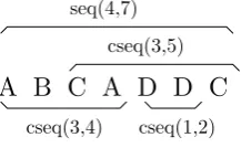
leads to a so-calledstack distance profile, as it is depicted in figure 2. The stack distance profile characterizes the positions of cache lines on the LRU stack when accessing cache data.
Cα
C1 Cα+1
n
u
m
b
er of access
stack distance counters
cache hits extra cache misses under cache sharing
original cache misses
[image:2.595.319.518.239.365.2]Cα
Figure 2: Stack distance histogram.
Given a stack distance profile, the total number of ac-cesses to a specific cache set can simply be determined by summing up allCi according to
accesses=
α+1 i=1
Ci (1)
and the cache miss rate can be calculated by
Pmiss= Cαα+1+1
i=1 Ci
. (2)
For a smaller cache with lower associativityα, the miss rate can be computed as
Pmiss(α) = Cα+1+ α
i=αCi
α+1
i=1 Ci
. (3)
Chandra et al. exploit this equation to predict the cache miss rate under cache sharing. They estimate the effec-tive associativityαof a task when sharing the cache with another task according to
α= effCacheSizex
numCacheSets, (4)
where numCacheSets denotes the number of sets the cache is composed of and effCacheSizex the effective cache size that is available for threadx.
Within their FOA model, they calculate the effective cache size according to
effCacheSizex=
α+1
i=1 Ci,x
N y=1
α+1
i=1 Ci,y
Within their SDC model, they create a new stack dis-tance profile by merging individual stack disdis-tance profiles to one profile and determine the effective cache space for each thread “proportionally to the number of stack dis-tance counters that are included in the merged profile.”[1]
The shaded region in figure 2 shows how the effective cache size is reduced by cache sharing.
While theFOA and the SDC model both are heuristic models, Chandra et al. also developed an inductive prob-ability model that is based on circular sequences rather than on stack distances.
2.3
Chandra
et
al.’s
Circular
Sequence
Based Prob Method
Circular sequences are an extension to stack distances in that they do not only take into account the number of accesses to the different positions on the LRU stack, but also the number of cache accesses between accesses to equal positions on the LRU stack.
Therefore, Chandra et al. define asequence seqx(dx, nx)
as “a series of nx cache accesses to dx distinct line
ad-dresses by thread x, where all the accesses map to the same cache set” [1] and acircular sequence cseq(dx, nx)
as a sequence seqx(dx, nx) “where the first and the last
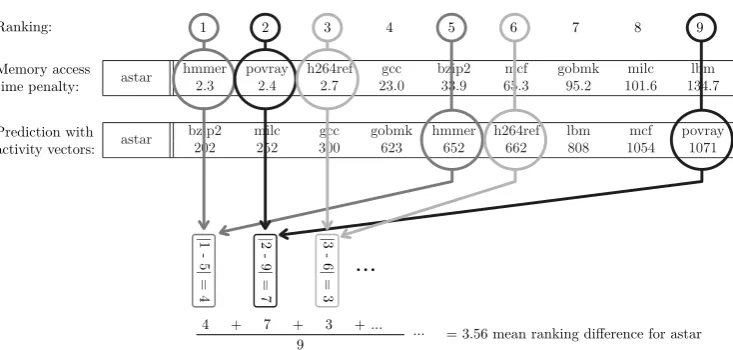
accesses are to the same line and there are no other ac-cesses to that address” [1]. Circular sequences can be regarded as stack distances that have each counterC aug-mented with an additional vectorn to hold a histogram of accesses for each distance. Figure 3 illustrates the rela-tionship between sequences and circular sequences when accessing cache linesA,B,CandD.
A B C A D D C
cseq(1,2) cseq(3,4)
[image:3.595.108.217.523.590.2]cseq(3,5) seq(4,7)
Figure 3: Relationship between sequences and circular sequences. A, B,C andDdepict different cache lines.
For their circular sequence based Prob model, Chandra et al. compute the number of cache misses for a thread x when sharing the cache with an additional thread y by adding to the stand-alone cache missesCα+1 the val-ues of the other countersC1. . . Cα, each multiplied with
the probability that the corresponding circular sequences cseq(dx, nx) will become a miss, wherenxcorresponds to
the estimatedmean n for a specificd:
missx=Cα+1+ α
dx=1
Pmiss(cseqx(dx, nx))×Cdx (6)
Chandra et al. calculate the probability that the circular sequencecseq(dx, nx)) will become a miss by summing up
the probabilities that there are sequencesseqy(dy, E(ny))
in thready withα−dx+ 1≤dy ≤E(ny), where E(ny)
represents the expected value ofnin the thready:
Pmiss(cseqx(dx, nx)) =
E(ny)
dy=α−dx+1
P(seqy(dy, E(ny)))
(7) E(ny) is estimated by scaling nx proportionally to the
ratio of accesses ofy andx:
E(ny) =
α+1
i=1 Ciy α+1
i=1 Cix
·nx (8)
The probability of sequencesP(seqy(dy, E(ny))), in short
P(seq(d, n)), is calculated recursively according to
if if if
if
where P(d−) = di=1P(cseq(i,∗)) and P(d+) = 1− P(d−) (cgf. [1]) and the asterisk (∗) incseq(i,∗) denotes all possible values.
3
Setvector
Based
Cache
Contention
Prediction
In this section, we describe our setvector method. First, we present the algorithm to obtain setvectors. Second, we show how setvectors can be used to predict cache con-tention.
3.1
Generating Setvectors
Setvectors are composed of cache set access frequencies
a and the number of different cache lines d referenced within a specific amount of time, typically about an op-erating system’s timeslice. Within this paper, we collect one setvector for every interval at 220 instructions. Ac-cording to our proposal in [9] where we presented setvec-tors to predict L2 cache performance of stand-alone ap-plications, we assume an L2 cache with 32 bit address length that usesb bits to code the byte offset, s bits to code the selection of the cache set and k = 32−s−b bits to code thekey that has to be compared to the tags stored in the tag RAM. The setvectors are gathered as follows:
For every intervaliof 220 instructions do:
• First, set the 1×2s sized vectorsaanddto0.
– Extract the set number from the address, e.g. by shifting the address k bits to the left and then unsigned-shifting the result k+b bits to the right.
– Extract the key from the address, e.g. by un-signed shifting the addresss+bbits to the right.
– Increasea[set number].
– In the list of the given set, determine whether the given key is already present.
– If the key is already present, do nothing and proceed with the next address.
– If the key is not in the list yet, add the key and increased[set number].
We end up with two 1×2sdimensional vectorsaand
d. At indexj, a holds the number of references to set j and dholds the number of memory references that map to set j, but provide a different key.
• In a third step, subtract the cache associativity α from each element indand store the result ind. If the result gets negative, store 0 instead.
• In a forth step, multiply each element ofa with the corresponding element in d and store the result in the 1×2s dimensional setvectors
i.
• Finally, add si as the ith column of matrix Sthat
holds in each column ithe setvector for intervali.
Process next interval.
3.2
Predicting
Cache
Contention
with
Setvectors
The compatibility of two threads for a time intervalican easily be predicted by just extractingsixfromSxandsiy
from Sy and calculating the dot product six·siy of the setvectors in order to obtain a single value. A low valued dotproduct implies a good match of the applications, a high dotproduct value suggests a bad match, i.e. a high level of cache interference resulting in many cache misses.
The dotproducts do not have any specific meaning like number of additional cache misses, as it is the case with Chandra’s circular sequence based method. However, comparing the dotproducts of several thread combina-tions in relation to each other has been proven to be an effective way to predict which threads make a better match and which threads do not.
4
Evaluating Cache Contention
Predic-tion Techniques – SimulaPredic-tion Setup
In order to prove the effectiveness of the setvector method with its relative comparison of dotproducts, we com-pared it to Settle’s activity vector method and to Chan-dra’s circular sequence based method. We refrained from
additionally comparing the setvector method to Chan-dra’s stack distance based method, as Chandra already reported that the circular sequence based method out-performed the stack distance based methods – and our setvector method showed nearly the same accuracy as the circular sequence based method.
To compare and evaluate the cache contention prediction techniques, we generated tracefiles with memory accesses representing 512 million instructions for each of the ten SPEC2006 benchmark programsastar,bzip2,gcc,gobmk, h264ref,hmmer,lbm,mcf,milcand povray applying the Pin toolkit [4]. Of these ten programs, we executed ev-ery 45 pairwise combinations on our MCCCSim multicore cache contention simulator [8] that had been parameter-ized as follows:
Parameter private L1 cache shared L2 cache
Size 32 k 2 MB
Line size 128 Byte 128 Byte
Associativity 2 8
Hit time 1.0 ns 10.0 ns
Miss time depends on L2 100.0 ns
Replacement LRU LRU
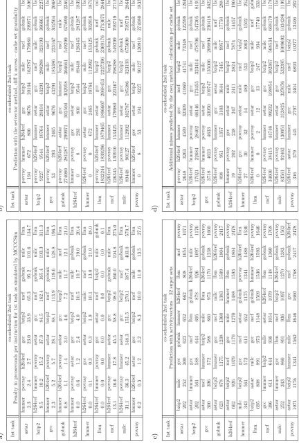
For each program of each combination, we calculated the difference between the stand-alone memory access time and the memory access time when executed in co-schedule with the other application. From this difference, we calculated the additional penalty in picoseconds per instruction, that is shown for every combination in table 3a). Additionally, we sorted the results according to 1st) this penalty and 2nd) the application’s name.
Then, we calculated the predictions for theactivity vector method, Chandra’scircular sequence based method and oursetvectormethod and sorted them accordingly, as can be seen from table 3b) - 3d).
To evaluate the prediction methods, we introduce a method we callmean ranking difference(MRD): We com-pare the rows of table 3a) that represent values gath-ered from MCCCSim with those of the predictions, ex-emplarily shown in table 3b) - 3d). Figure 4 shows that we calculate the absolute difference between the position (ranking) determined by MCCCSim and the position de-termined by the prediction for each combination. The results are summed up and divided by the total num-ber of co-scheduled applications (9) to yield the average mean ranking distance (MRD), i.e. the mean number of positions, a co-schedule’s prediction differs from the real values obtained from MCCCSim.
We evaluated several variations of all three methods.
astar hmmer povray h264ref gcc bzip2 mcf gobmk milc lbm
2.3 2.4 2.7 23.0 33.9 65.3 95.2 101.6 134.7
astar bzip2 milc gcc gobmk hmmer h264ref lbm mcf povray
202 252 300 623 652 662 808 1054 1071
Memory access time penalty:
Prediction with activity vectors:
[image:5.595.106.473.91.266.2]Ranking: 1 2 3 4 5 6 7 8 9
|1 - 5| = 4 |2 - 9| = 7 |3 - 6| = 3
...
4 + 7 + 3 + ...
9
... = 3.56 mean ranking difference for astar
Figure 4: Determination of the mean ranking difference (MRD) forastar.
• Chandra cseq chunkset: Prediction while applying only one circular sequence stack to a chunkset (i.e. interval of 220 instructions).
• Chandra cseq Af(set): Prediction while applying a circular sequence stack to every cache set within an interval and measuring the memory access frequency on a per cache set basis.
• Chandra cseq Af(chunkset): Prediction while ap-plying a circular sequence stack to every cache set within an interval without partitioning the memory access frequency on the cache sets, i.e. providing only one memory access frequency value per inter-val.
Settle et al. stated that “the low order bits of the cache set component of a memory address are used to index the activity counter associated with each cache super set.” [6] However, we expected that the method would achieve better results when using thehighorder bits to index the activity counters since addresses with equal high order bits are mapped to equal cache sets. Therefore, we eval-uated the activity vector method for these two variants naming themhigh respectivelylow (cf. table 1).
With the setvector method, we were interested in analyz-ing the followanalyz-ing variations (cf. table 1):
• diff. x access: The setvector method as it had been presented in chapter 3.
• access: Utilizing only the access frequency. This way, the performance of the activity vector method can be estimated for the case that the number of su-persets reaches its maximum (i.e. the over all num-ber of sets) and the activity expresses the numnum-ber of accesses to a set and not just the one-bit infor-mation, whether or not a specific threshold has been reached.
• diff: Utilizing only the number of different cache
lines that are mapped to the same cache set, i.e. ignoring any access frequency.
• add, mul: Combining the vectors of two threads by applying either elementwise addition or multiplica-tion and calculating the average of the elements af-terwards, rather than by applying the dot product.
5
Results
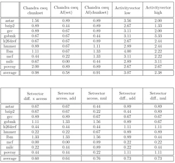
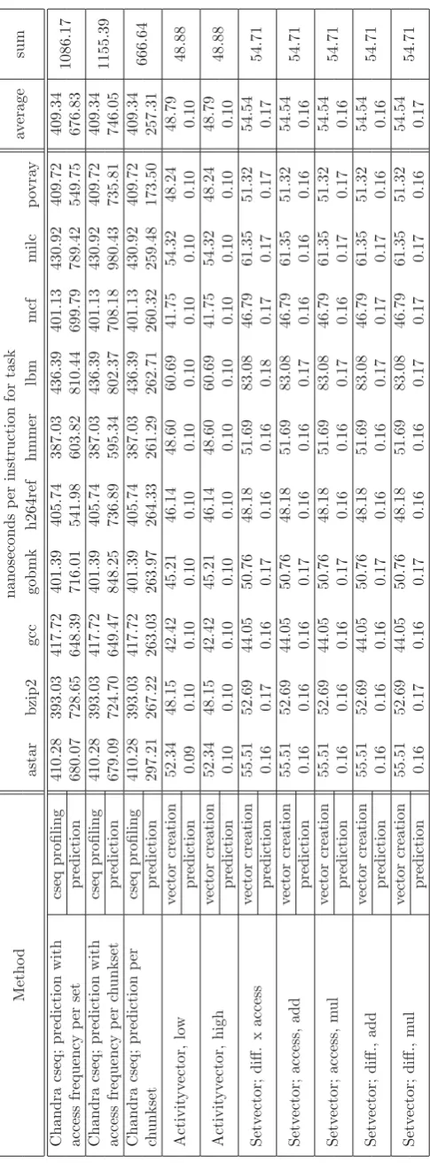
Table 1 shows the accuracy of the evaluated methods and variations, table 2 shows the execution time of the meth-ods, subdivided into time that has to be spend offline (rowcseq profilingandvector creation), and the time that has to be spendonline(rowprediction) when calculating the prediction for a specific combination. Table 1 shows that Chandra’s circular sequence based method that uti-lizes the access frequency on aper set basis performs with the highest accuracy (M RD = 0.58). However, 676.83 picoseconds have to be spent per instruction (ps/instr.) on average to calculate the predictions, i.e. prediction takes about 6768 times longer than for the activity vec-tor method (0.10 ps/instr.) and about 3981 times longer as for the setvector method.
Although the activity vector method performs quite fast, it shows a high error rate (M RD = 3.07 and M RD = 2.38 respectively). However, selecting the higher part of the set bits had been a good idea. Increasing the number of super sets to the number of sets and applying natu-ral numbers to count the number of accesses to each set instead of using only a single bit per set significantly im-proves accuracy (M RD= 0.64, as seen fromSetvector – access, add), but also increases prediction time (0.16).
Chandra cseq chunkset
Chandra cseq Af(set)
Chandra cseq Af(chunkset)
Activityvector low
Activityvector high
astar 1.56 0.89 0.89 3.56 2.00
bzip2 0.89 0.44 0.89 2.67 1.33
gcc 0.89 0.67 0.89 3.11 2.00
gobmk 0.67 0.67 0.44 3.11 3.33
h264ref 0.67 0.67 0.89 2.67 2.44
hmmer 0.89 0.67 1.11 2.89 2.44
lbm 1.11 0.67 1.33 4.00 2.22
mcf 0.44 0.22 1.33 3.11 2.22
milc 0.67 0.00 0.44 2.89 3.11
povray 2.00 0.89 0.89 2.67 2.67
average 0.98 0.58 0.91 3.07 2.38
Setvector diff. x access
Setvector access, add
Setvector access, mul
Setvector diff., add
Setvector diff., mul
astar 0.67 0.67 0.44 0.89 0.89
bzip2 0.67 0.67 0.22 0.44 0.89
gcc 0.89 0.89 0.67 0.67 0.67
gobmk 1.11 1.33 1.56 0.89 0.67
h264ref 0.44 0.44 0.44 1.11 1.11
hmmer 0.22 0.22 0.67 0.89 0.89
lbm 1.33 1.33 1.56 0.89 0.44
mcf 0.00 0.00 0.89 0.22 0.22
milc 0.22 0.44 0.89 0.22 0.44
povray 0.44 0.44 0.22 1.11 1.11
[image:6.595.120.463.94.412.2]average 0.60 0.64 0.76 0.73 0.73
Table 1: Mean ranking difference (MRD) for each benchmark and method.
6
Conclusion
In this paper, we presented state-of-the art methods to predict cache contention and proposed a new predic-tion method based on the calculapredic-tion of so-called setvec-tors. We simulated the additional memory access time introduced by cache contention during application co-scheduling and compared those values to the prediction methods by applying a new metric called MRD (mean ranking distance) that calculates the mean difference be-tween the predicted and the simulated ranking.
Our results showed that the method introduced by Chan-dra et al. [1] might be the most accurate one, but it is nearly 4000 times slower than the proposed setvec-tor method, that achieves nearly the same accuracy (M RD= 0.60 instead ofM RD= 0.58).
References
[1] D. Chandra, F. Guo, S. Kim, and Y. Solihin. Predicting Inter-Thread Cache Contention on a Chip Multi-Processor Architecture. Proceedings of the 11th Int’l Symposium on High-Performance Computer Architecture (HPCA-11 2005), 2005.
[2] A. Fedorova. Operating System Scheduling for Chip Mul-tithreaded Processors. PhD thesis, Harvard University, Cambridge, Massachusetts, 2006.
[3] M. D. Hill and A. J. Smith. Evaluating Associativity in CPU Caches. InIEEE Transactions on Computers, vol-ume 38, 1989.
[4] C.-K. Luk, R. Cohn, R. Muth, H. Patil, A. Klausner, G. Lowney, S. Wallace, V. J. Reddi, and K. Hazelwood. Pin: Building Customized Program Analysis Tools with Dynamic Instrumentation. InProgramming Language De-sign and Implementation, ACM, 2005.
[5] R. L. Mattson, J. Gecsei, D. R. Slutz, and I. L. Traiger. Evaluation Techniques for Storage Hierarchies. In IBM Systems Journal, volume 9, 1970.
[6] A. Settle, J. L. Kihm, A. Janiszewski, and D. A. Connors. Architectural Support for Enhanced SMT Job Scheduling.
Proceedings of the 13th International Conference of Paral-lel Architectures and Compilation Techniques, September 2004.
[7] W. A. Wulf and S. A. McKee. Hitting the Memory Wall: Implications of the Obvious.Computer Architecture News, 23(1), March 1995.
[8] M. Zwick, M. Durkovic, F. Obermeier, W.
Bam-berger, and K. Diepold. MCCCSim - A Highly
Configurable Multi Core Cache Contention Simulator.
Technical Report - Technische Universit¨at M¨unchen, https://mediatum2.ub.tum.de/doc/802638/802638.pdf, 2009.
Metho
d
nanoseconds
p
er
instruction
for
task
a
v
erage
sum
astar
bzip2
gcc
gobmk
h264ref
hmmer
lbm
mcf
milc
p
o
vra
y
Chandra
cseq;
prediction
with
access
frequency
p
er
set
cseq
profiling
410.28
393.03
417.72
401.39
405.74
387.03
436.39
401.13
430.92
409.72
409.34
1086.17
prediction
680.07
728.65
648.39
716.01
541.98
603.82
810.44
699.79
789.42
549.75
676.83
Chandra
cseq;
prediction
with
access
frequency
p
er
ch
unkset
cseq
profiling
410.28
393.03
417.72
401.39
405.74
387.03
436.39
401.13
430.92
409.72
409.34
1155.39
prediction
679.09
724.70
649.47
848.25
736.89
595.34
802.37
708.18
980.43
735.81
746.05
Chandra
cseq;
prediction
p
er
ch
unkset
cseq
profiling
410.28
393.03
417.72
401.39
405.74
387.03
436.39
401.13
430.92
409.72
409.34
666.64
prediction
297.21
267.22
263.03
263.97
264.33
261.29
262.71
260.32
259.48
173.50
257.31
Activit
yv
ector,
lo
w
v
ector
creation
52.34
48.15
42.42
45.21
46.14
48.60
60.69
41.75
54.32
48.24
48.79
48.88
prediction
0.09
0.10
0.10
0.10
0.10
0.10
0.10
0.10
0.10
0.10
0.10
Activit
yv
ector,
high
v
ector
creation
52.34
48.15
42.42
45.21
46.14
48.60
60.69
41.75
54.32
48.24
48.79
48.88
prediction
0.10
0.10
0.10
0.10
0.10
0.10
0.10
0.10
0.10
0.10
0.10
Setv
ector;
diff.
x
access
v
ector
creation
55.51
52.69
44.05
50.76
48.18
51.69
83.08
46.79
61.35
51.32
54.54
54.71
prediction
0.16
0.17
0.16
0.17
0.16
0.16
0.18
0.17
0.17
0.17
0.17
Setv
ector;
access,
add
v
ector
creation
55.51
52.69
44.05
50.76
48.18
51.69
83.08
46.79
61.35
51.32
54.54
54.71
prediction
0.16
0.16
0.16
0.17
0.16
0.16
0.17
0.16
0.16
0.16
0.16
Setv
ector;
access,
m
u
l
v
ector
creation
55.51
52.69
44.05
50.76
48.18
51.69
83.08
46.79
61.35
51.32
54.54
54.71
prediction
0.16
0.16
0.16
0.17
0.16
0.16
0.17
0.16
0.17
0.17
0.16
Setv
ector;
diff.,
add
v
ector
creation
55.51
52.69
44.05
50.76
48.18
51.69
83.08
46.79
61.35
51.32
54.54
54.71
prediction
0.16
0.16
0.16
0.17
0.16
0.16
0.17
0.17
0.17
0.16
0.16
Setv
ector;
diff.,
m
u
l
v
ector
creation
55.51
52.69
44.05
50.76
48.18
51.69
83.08
46.79
61.35
51.32
54.54
54.71
prediction
0.16
0.17
0.16
0.17
0.16
0.16
0.17
0.17
0.17
0.16
[image:7.595.170.413.98.755.2]0.17
1st task co-sc heduled 2nd task Additional misses predicted b y the cseq metho d – calculation p er cac he set astar p o vra y h264ref hmmer gcc mcf bzip2 milc gobmk lbm 2648 3263 4509 32309 41069 41741 73348 122598 126190 bzip2 h264ref hmmer p o vra y astar gcc milc mcf gobmk lbm 17021 22684 28402 66146 173455 323414 478706 547305 819350 gcc h264ref hmmer p o vra y astar bzip2 milc mcf gobmk lbm 3718 4623 4633 33950 109747 135006 209894 230418 362239 gobmk h264ref p o vra y hmmer gcc astar bzip2 milc mcf lbm 898 951 1357 3103 3644 7445 9957 17750 28811 h264ref hmmer p o vra y gcc astar milc bzip2 mcf gobmk lbm 19 202 238 247 2411 3824 7874 14457 19004 hmmer h264ref gcc p o vra y astar milc mcf bzip2 gobmk lbm 27 30 32 54 489 533 1003 1502 2524 lbm h264ref hmmer p o vra y astar gcc bzip2 milc mcf gobmk 0 0 2 12 13 247 934 17740 33327 mcf h264ref p o vra y hmmer astar gcc bzip2 milc gobmk lbm 34600 38415 44746 99232 168854 302367 568534 668179 1178915 milc h264ref p o vra y hmmer astar gcc bzip2 mcf gobmk lbm 83561 92462 130951 313825 327676 532395 1009692 1034280 1199336 po v ra y h264ref astar hmmer gcc milc mcf bzip2 gobmk lbm 316 379 445 2797 3404 6893 10277 12406 29227 1st task co-sc heduled 2nd task P enalt y in picoseconds p er instruction for 1st task as sim ulated b y MCCCSim astar hmmer p o vra y h264ref gcc bzip2 mcf gobmk milc lbm 2.3 2.4 2.7 23.0 33.9 65.3 95.2 101.6 134.7 bzip2 h264ref hmmer p o vra y astar gcc mcf gobmk milc lbm 9.5 10.2 15.2 37.3 84.5 162.4 165.4 193.3 311.3 gcc hmmer h264ref p o vra y astar bzip2 mcf gobmk milc lbm 2.3 5.2 5.7 28.1 88.1 113.9 119.6 128.8 196.5 gobmk hmmer h264ref p o vra y astar gcc bzip2 milc mcf lbm 0.8 1.1 1.4 3.0 4.6 7.2 11.7 12.1 21.0 h264ref hmmer p o vra y astar gcc bzip2 mcf milc gobmk lbm 0.0 0.6 1.2 2.4 4.0 10.5 10.7 19.0 20.4 hmmer h264ref p o vra y gcc astar bzip2 milc mcf gobmk lbm 0.0 0.1 0.3 0.3 1.9 10.1 13.0 21.0 48.0 lbm h264ref hmmer p o vra y gcc astar mcf bzip2 milc gobmk 0.0 0.0 0.0 0.0 0.0 0.0 0.0 0.0 0.1 mcf h264ref p o vra y hmmer astar gcc bzip2 gobmk milc lbm 13.1 16.6 17.8 45.5 58.8 98.6 160.0 194.8 275.0 milc h264ref p o vra y hmmer astar gcc bzip2 mcf gobmk lbm 31.1 36.3 45.2 148.3 151.5 270.1 387.4 403.0 570.7 po v ra y hmmer h264ref astar gcc bzip2 mcf milc gobmk lbm 0.2 0.3 1.2 3.2 8.3 10.0 11.0 13.5 27.6 1st task co-sc heduled 2nd task Prediction with activit yv ectors – 3 2 sup er sets astar bzip2 milc gcc gobmk hmmer h264ref lbm mcf p o vra y 202 252 300 623 652 662 808 1054 1071 bzip2 astar hmmer gcc mcf lbm gobmk h264ref milc p o vra y 202 561 588 644 695 878 926 1097 1176 gcc astar mcf hmmer bzip2 milc lbm h264ref gobmk p o vra y 300 396 572 588 860 973 1170 1238 1660 gobmk astar bzip2 hmmer gcc mcf milc lbm h264ref p o vra y 623 878 1175 1238 1360 1383 1509 1804 2417 h264ref astar bzip2 mcf gcc milc hmmer lbm gobmk p o vra y 662 926 1079 1170 1270 1488 1593 1804 2478 hmmer milc bzip2 gcc mcf astar gobmk p o vra y h264ref lbm 343 561 572 611 652 1175 1341 1488 1536 lbm bzip2 astar milc gcc mcf gobmk hmmer h264ref p o vra y 695 808 891 973 1148 1509 1536 1593 1646 mcf gcc hmmer bzip2 milc astar h264ref lbm gobmk p o vra y 396 611 644 936 1054 1079 1148 1360 1768 milc astar hmmer gcc lbm mcf bzip2 h264ref gobmk p o vra y 252 343 860 891 936 1097 1270 1383 1562 po v ra y astar bzip2 hmmer milc lbm gcc mcf gobmk h264ref 1071 1176 1341 1562 1646 1660 1768 2417 2478 1st task co-sc heduled 2nd task Prediction with the setv ector metho d, diff x access – cac he set gran ularit y astar p o vra y hmmer h264ref gcc bzip2 milc mcf gobmk lbm 194 672 800 9676 20104 162787 179980 299971 1896607 bzip2 p o vra y h264ref hmmer astar gcc mcf milc gobmk lbm 9227 9544 10764 20104 43291 298288 323193 366661 2227396 gcc p o vra y h264ref hmmer astar bzip2 milc mcf gobmk lbm 53 293 2465 9676 43291 185386 223167 302504 2068453 gobmk p o vra y h264ref astar gcc hmmer bzip2 mcf milc lbm 274080 281287 299971 302504 302958 366661 549299 675690 2369176 h264ref hmmer p o vra y gcc astar bzip2 milc mcf gobmk lbm 0 8 293 800 9544 89448 126345 281287 1839296 hmmer h264ref p o vra y astar gcc bzip2 milc mcf gobmk lbm 0 0 672 2465 10764 112992 153425 302958 1879465 lbm p o vra y h264ref hmmer astar gcc bzip2 gobmk mcf milc 1833244 1839296 1879465 1896607 2068453 2227396 2369176 2713675 2864029 mcf h264ref p o vra y hmmer astar gcc bzip2 gobmk milc lbm 126345 130910 153425 179980 223167 298288 549299 709719 2713675 milc h264ref p o vra y hmmer astar gcc bzip2 gobmk mcf lbm 89448 90127 112992 162787 185386 323193 675690 709719 2864029 po v ra y hmmer h264ref gcc astar bzip2 milc mcf gobmk lbm 0 8 53 194 9227 90127 130910 274080 1833244 a) b) c) d)