Predicting River Pollution Using Random Forest Decision Tree with GIS Model: A Case Study of MMORS, Philippines

(1)



Abstract—This study aims to predict the pollution level that

threatens the Marilao-Meycauayan-Obando River System (MMORS), located in the province of Bulacan, Philippines. The inhabitants of this area are now being exposed to pollution. Contamination of this waterway comes from both formal and informal industries, such as a used lead-acid battery, open dumpsites metal refining, and other toxic metals. Using various water quality parameters like Dissolved Oxygen (DO), Potential of Hydrogen (pH), Biochemical Oxygen Demand (BOD), Total Suspended Solids (TSS), Nitrate, Phosphate, and Coliform are the basis for predicting the pollution level. Base on the sample data collected from January 2013 to May 2018. These are used as a training data and test results to predict the river condition with its corresponding pollution level classification indicated. Random Forest decision tree model got an accuracy of 99.38% with a Kappa value of 0.8303 interpreted as “Strong” in terms of the level of agreement and GIS model shows the heat map of the different water quality parameter and Water Quality Index (WQI) spatial distribution, the majority of the sampling station are greatly polluted provided that they have „Poor‟ and ‟Very Poor.‟

Index Terms—Machine learning, river pollution, random

forest and GIS.

I. INTRODUCTION

In the Philippines, Marilao-Meycauayan-Obando River System (MMORS) is included in the ―World‘s Worst Polluted Places‖ as reported by PureEarth formerly known as Blacksmith Institute [1]. Aside from organic pollution, there are abundances of heavy metal that may pose significant health risks to surrounding communities that depend on the river system. According to Malenab et al. [2],heavy metal pollution came from used jewelry smelting, tanneries, used lead-acid battery recycling and other industries dealing with heavy metals commonly in the upstream area of the river system. These pollutants, especially the heavy metals, pose a significant health risk to nearby communities that surround the river water for fish ponds, bathing, and swimming that causes some health concerns and in addition, 31% of all illnesses in the country are attributed to polluted waters. An average of 55 Filipinos per day suffers from diseases attributed to poor sanitation and poor water quality. There are

Manuscript received June 22, 2019; revised November 13, 2019. J. M. Victoriano is with Bulacan State University, City of Malolos, Bulacan, Philippines. He is also with AMA University Quezon City, Philippines (e-mail: [email protected]).

L. L. Lacatan is with the College of Engineering at AMA, University Quezon City, Philippines (e-mail: [email protected]).

A. A. Vinluan is with AMA University Quezon, City Philippines (e-mail: [email protected]).

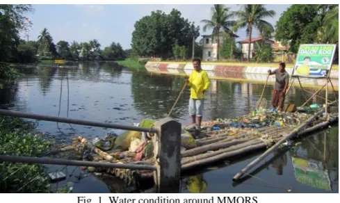
several attempts to rehabilitate the aforesaid river system and the noteworthy one that may be credited to the MMORS rehabilitation actions is the compliance of many industries, which began in 2008, with DENR declaring the river system as a Water Quality Management Area (WQMA). With funding from the Japan International Cooperation Agency (JICA) [2] and support from NGOs such as the Blacksmith Institute, a New York-based non-profit organization, Fig. 1 shows the observed condition of MMORS as the result of river quality monitoring since 2005.

Fig. 1. Water condition around MMORS.

The Data (water parameter result) Dissolve Oxygen (DO), Potential Hydrogen(pH), Biochemical Oxygen Demand(BOD), Total Suspended Solid(TSS), Nitrate, Phosphate, and Coliform that are being collected from January 2013 to May 2018 are used as training set and test set to decide the accuracy of the predictive model and help the Local Government Unit (LGU) of MMORS and its municipal communities in providing awareness and consciousness about the MMORS pollution level. Fig. 2 shows the Map of MMORS and its sampling Station covering around 55 kilometers from upstream Caloocan down to Manila Bay.

There are two main objectives solved in this case study. The first is to predict pollution level using Random Forest (RF) Decision Tree which provides the most accurate forecast and the second - visualize heatmap area through Geographic Information System model using Kernel Density Estimation KDE Heat Map.

II. PROCEDURE

A. Study Area

The study is conducted in three coastal municipalities in Bulacan (Fig. 2). Thirteen sampling stations comprising of almost five barangays in Marilao, another five barangays in Meycauayan and three nearby areas in Obando, all in the

Predicting River Pollution Using Random Forest Decision

Tree with GIS Model: A Case Study of MMORS,

Philippines

(2)

province of Bulacan, Philippines are included in the study using cluster sampling design.

Fig 2. Study area — MMORS.

B. Preprocessing

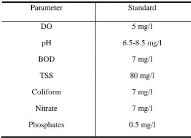
The collected dataset is based on the Department of Environment and Natural Resources (DENR) Environment Management Board (EMB) Region 3 starting from January 2013 to May 2018. This included the different water parameters and standards as shown in Table II. The author focused on DO, pH, BOD, TSS, Nitrate, Phosphate, and Coliform that measures an approximate amount of biodegradable organic matter present in water is generally used as the criterion to measure in determining the water quality of the river. Based on Water Quality Guideline of DENR Administrative Order, MMORS is classified as Type C body of water [3].

C. Water Quality Index

Using various water quality parameter and for the purposes of this study is calculated following three steps. For the first step, a weight ( ) is assigned to each of the seven parameters according to its relative importance in the overall quality of water for drinking. For the second step, the relative weight (Wi) is computed shown in equation 1:

(1)

where: ( ) is the relative weight, ( ) is the weight for each parameter and (n) is the number of parameters. For the third step, a quality rating scale ( ) for each parameter is assigned by dividing its concentration in each water sample by its respective standard and the result is multiplied by 100 to express it in percentage showed in equation 2.

(2) where: (qi) is the quality rating, (ci) is the concentration of each pollutant in water sample in mg/l, (Si). For computing the WQI, the Si is determined for each chemical parameter. The sub index of ith quality parameter can be determined by presented in equation 3:

(3)

D. Training and Test

This section describes what tools the researcher used in training and the supplied training data. This paper applied the Waikato Environment for Knowledge Analysis (WEKA). Random Forest Decision Tree is also used during the training process to provide a prediction with 10-fold cross-validation to avoid overfitting and to get a more accurate result [5]. Collected data started from January 2013 to May 2018 with a total of 650 instances.

TABLE II: WATER PARAMETER AND STANDARD

Parameter Standard

DO 5 mg/l

pH 6.5-8.5 mg/l

BOD 7 mg/l

TSS 80 mg/l

Coliform 7 mg/l

Nitrate 7 mg/l

Phosphates 0.5 mg/l

TABLE III: GENERAL DESCRIPTION OF THE CALCULATED WATER QUALITY RANK ADAPTED FROM THE CANADIAN COUNCIL OF MINISTERS OF THE

ENVIRONMENT [4]. WQI Value Water Quality

>=90 Excellent

>=70 Good

>=50 Poor

>=25 Very Poor >=0 Worst

The Random Forest algorithm process as shown below,

Random Forest works by building decision trees from a bootstrapped sample taken from a training set. This process is repeated B several times where B is the desired number of trees generated for the forest [6], [7]. During the construction of a tree, a node is split based on the best among the random subset of the features

Algorithm: Random Forest Decision Tree

Input: Let X be the training data consisting of L variable feature vectors.

Let B be the number of trees in a Random Forest.

Random Forest Training

1. For i =1, . . . . , B, iterate until convergence: (a) Draw a bootstrap sample S of size N from X. (b) Grow a tree from the bootstrapped data with the following conditions:

i. Given the L input variable, a number l << L is specified such that for each node. l variables are selected

randomly from X and the best split from l is used to split the node.

ii. Grow the tree without pruning 2. Output the ensemble of trees * +

Random Forest Prediction

Let x be a feature vector of a test data, the prediction is given by :

(3)

3. ̂

( ) ( )

E. Prediction and Validation

Random Forest Decision Tree classification as the major learning algorithm implemented in this undertaking is further utilized as a training data and test results to predict the MMORS river condition with its corresponding water pollution level classification indicated as ―Excellent‖, ―Good‖, ―Poor‖, ―Very Poor, and ―Worst‖ This section describes the different metrics used by the researcher in evaluating the classifier model performance [8]; its effectiveness and the quality of its prediction. Several tests of data with known water quality parameter values are used to test the accuracy of the generated sample by distinguishing the reliability of the data and their validity in accordance to the comparison of an observed accuracy with an expected accuracy rate that is likely to meet based on the Confusion Matrix [9]. The classifier can also be evaluated in terms of Precision, Recall, and F-measure and the assessment of interrater-reliability [10] .Cohen's Kappa is used which is shown in Table IV.

Precision is the ratio of relevant instances in the retrieved instances that are referred to as a positive value. Precision is calculated as shown in equation 4 where tp is truly positive and fp is a false-positive.

( ) (4) Recall it is defined as the true positive rate to calculate recall equation 5 must be used, where tp is true positive and fn is a false negative.

( ) (5) F-measureis the weighted average of Precision and Recall and is calculated as shown in equation 6.

( )

( ) (6) Interrater Reliability is to measure interrater reliability between two raters, Cohen's Kappa statistic is used which is shown in equation 7, where Po is the relative observed agreement among raters, Pe is the hypothetical probability of chance agreement and K is the Kappa value.

( )

(7) TABLE IV: KAPPA VALUE AND LEVEL OF AGREEMENT [10]

Value of Kappa Level of Agreement

0-.20 None

.21-.39 Minimal

.40-.59 Weak

.60-.79 Moderate .80-.90 Strong Above .90 Almost Perfect

F. Geographic Information System Model

Geographic Information System (GIS) is a computer-based information system used to digitally

represent and analyze the geographic features present on the Earth surface. GIS technology integrates common database operations such as query and statistical analysis with the unique visualization and geographic analysis benefits offered by maps [11]. Also, it is used to digitally reproduce and analyze the feature present on the earth surface and the events that take place on it.

There are many different mapping techniques that can be used for identifying and exploring patterns of water pollution [12] particularly in terms of water quality showed in Fig 4. In line with this, the researcher considers the Kernel Density Estimation (KDE) as the hotspot mapping technique to be used in predicting spatial patterns of pollution among the mapping techniques illustrated below.

Fig. 4. Common hotspot mapping techniques Common hotspot mapping techniques. (a) Point mapping, (b) choropleth thematic map, (c) grid thematic mapping, (d) standard deviational spatial ellipses and (e) KDE [13].

G. Kernel Density Estimation

There are a number of spatial analysis techniques that can be used for identifying hotspots, but the most popular in recent years is KDE [14], KDE is calculated by weighting the distances of all the data points for each location on the line. The concept of weighting the distances of observations from a particular point, , can be expressed mathematically using equation 8:

( ) (( ) (8) where K() is called the kernel function that is generally a

smooth, symmetric function such as a Gaussian and h > 0 is called the smoothing bandwidth that controls the amount of smoothing. Basically, the KDE smooths each data point Xi into small density bumps and then sum all these small bumps together to obtain the final density estimate.

III. RESULTS

(4)

International Journal of Environmental Science and Development, Vol. 11, No. 1, January 2020

in WEKA.

Another algorithm considered and tested is the Artificial Neural Network (ANN) which is based on a collection of connected units or nodes called artificial neurons, which loosely model the neurons in a biological brain. Each connection, like the synapses in a biological brain, can transmit a signal from one artificial neuron to another.

In the same manner, the k-nearest neighbor's algorithm (k-NN) is also considered and tested which is a

non-parametric method used for classification and regression.

The researcher also takes into consideration and test Naive Bayes which is a simple, yet effective and commonly-used, machine learning classifier.

Performance metrics considered including f-measure, recall, precision, Incorrectly classified Instance (ICI), Correctly Classified Instance (CCI), and Kappa Value. The result is shown in Table V.

TABLE V: MODEL PERFORMANCE COMPARISON WITH DIFFERENT METRICS

Classifier F-Measure Recall Precision ICI CCI Kappa Value

RF 0.993 0.994 0.994 0.62 99.38 0.830

J48 0.988 0.988 0.988 1.232 98.77 0.708

ANN 0.972 0.975 0.97 2.465 97.53 0.261

KNN 0.974 0.975 0.974 2.465 97.53 0.372

Naïve Bayes 0.959 0.945 0.984 5.547 94.45 0.417

As the result showed in Table V, RF decision tree achieved highest F-measure (0.993), reached the highest recall (0.994), realized the highest precision (0.994), and got the largest CCI (99.38) and Kappa Value (0.8303) respectively. Considering the Kappa table of interrater reliability shown in Table IV, the respective Kappa Value has a strong level of agreement. In this case, RF classifier performance is relatively high in almost all of the different metrics when compared with the other models.

The confusion matrix is constructed as showed in Table VI follows from the cross-validation prediction where diagonal entries represent correctly classified samples and the rest represent misclassifications. This enables us to visualize prediction results.

TABLE VI: CONFUSION MATRIX GENERATED BY RANDOM FOREST DECISION TREE

a b <--Classified as

636 0 a – Very Poor

5 9 b - Poor

The True Positive (TP) Rate, False Positive (FP) Rate, Precision, Recall, and F-Measure values are used. The rates Random Forest Decision Tree methods are shown in Table VII. of detailed accuracy by class.

TABLE VII: DETAILED ACCURACY BY CLASS CLASS TP

RATE FP RATE

PRECISION RECALL F-MEASURE

VERY POOR

1.00 0.286 0.994 1.000 0.997

POOR 0.714 0.000 1.000 0.714 0.833 WEIGHTED

AVERAGE

0.994 0.280 0.994 0.994 0.993

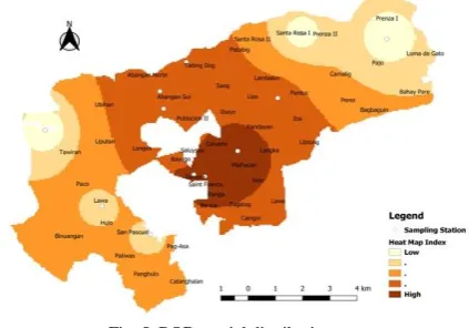
Biochemical oxygen demand or BOD is a chemical procedure for determining the amount of dissolved oxygen needed by aerobic biological organisms in a body of water to break down organic material present in a given water sample at certain temperature over a specific time period.

Fig. 5 shows the spatial distribution of BOD generated using GIS model. There is a clear variation at some point in the heat map considering each of the sampling stations. It is evident in the distribution that there is indeed a gradual decrease and increase of such substance when crossing the river system from both ends toward the center or the other

way around.

From Fig. 5, the BOD is low in most of the area of Marilao mainly in Santa Rosa I, Prenza I and II. The high concentration of BOD is found in the river areas of Malhacan, Zamora, Saint Francis and part of nearby sampling stations. This is above the desirable limit of BOD concentration in river water. BOD indicates the amount of putrescible organic matter present in water. Therefore, a low BOD is an indicator of good quality water, while a high BOD indicates polluted water.

Fig. 5. BOD spatial distribution.

Dissolved oxygen is the presence of these free O2 molecules within the water. The bonded oxygen molecule in water (H2O) is in a compound and does not count toward dissolved oxygen levels. One can imagine that free oxygen molecules dissolve in water much the way salt or sugar does when it is stirred.

The findings in this parameter show that the spatial distribution for Dissolve Oxygen fluctuates heavily in the extremities of MMORS in Fig. 6 with the aid of GIS. The substantial transition between the two is further expound in Fig. 6 where the water parameter set off greater intensity at the margins of the river system.

(5)

gas bubble disease in fish and invertebrates. Water with high concentrations of dissolved minerals such as salt will have a lower DO concentration than fresh water at the same temperature. Low dissolved oxygen (DO) primarily results from excessive algae growth caused by phosphorus. Nitrogen is another nutrient that can contribute to algae growth.

Fig. 6. DO spatial distribution.

Unlike temperature and dissolved oxygen, the presence of nitrates usually does not have a direct effect on aquatic insects or fish. However, excess levels of nitrates in water can create conditions that make it difficult for aquatic insects or fish to survive. Algae and other plants use nitrates as a source of food.

In this water quality parameter, the density estimates by means of spatial distribution drawn a quite difference which is patent in the next figure. Fig. 7 insinuates diminution of the water substance from the upper right borders of MMORS down to lower limits. This only denotes that this is one of the parameters that should be given much attention in undertaking water quality.

From Fig. 7, the nitrate concentration in the present study area of the river water within the permissible limit (<45mg/l). The nitrate concentration in between 45-100 mg/l is mostly in the sampling stations of Marilao like Loma De Gato, Camalig, Patubig, Santa Rosa II, Tabing Ilog, Abangan Norte, etc. Higher nitrate concentration of more than 100 mg/lit are found in areas like Santa Rosa I, Prenza I and II in Marilao which is very similar to the BOD level.

Fig. 7. Nitrates spatial distribution.

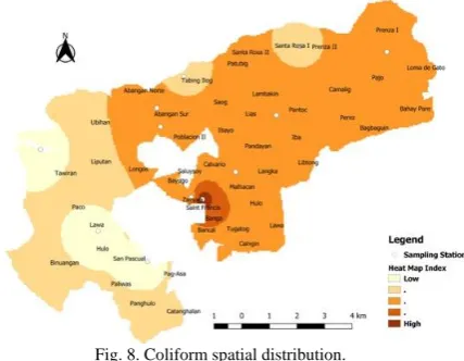
Coliform bacteria are present in the environment and feces of all warm-blooded animals and humans. Coliform bacteria are unlikely to cause illness. However, their presence in drinking water indicates that disease-causing organisms

(pathogens) could be in the water system.

Based on Fig. 8, the coliform spatial distribution alludes approximately half of water sampling stations are more or less polluted with this kind of substance. This only implies that the actual estimation for coliform and in reality, are not at far from each other therefore accuracy is achieved.

Fig. 8 shows, except Zamora, Saint Francis, and surrounding areas, the remaining stations of MMORS in terms of coliform water are somehow moderate and low. However, from the map below, predominantly areas river water quality within Marilao and Meycauayan are still doubtful. This would only indicate the potential presence of disease-causing bacteria in water. Furthermore, it might also indicate that human or animal waste is entering the water supply.

Fig. 8. Coliform spatial distribution.

The pH value is a good indicator of whether water is potable to drink or not. The pH of pure water is 7. In general, water with a pH lower than 7 is considered acidic, and with a pH greater than 7 is considered basic. The normal range for pH in surface water systems is 6.5 to 8.5, and the pH range for riverwater systems is between 6 to 8.5. Alkalinity is a measure of the capacity of the water to resist a change in pH that would tend to make the water more acidic. The measurement of alkalinity and pH is needed to determine the corrosiveness of the water.

To ascertain the pH using GIS, the researcher devised the spatial distribution which can be observed in Fig. 9 across all the sampling stations. In the same figure it can be seen that the spreading of this parameter intensifies as one moved to the edges of the map. This only reveals that there is a close association with this parameter and the other ones.

From Fig. 9, a considerable number of sampling stations in Obando and Marilao river areas such as Tawiran, Lawa, Loma De Gato, Santa Rosa I, Prenza I and II have above the permissible limit i.e. neutral pH of 7. The lower concentration of pH is found to be within the sampling stations largely in Meycauayan this only suggests that zero through 7 indicates acidity, the lower the number the higher the acidity. Consuming excessively acidic or alkaline water is harmful, warns the Environmental Protection Agency (EPA). Drinking water must have a pH value of 6.5-8.5 to fall within EPA standards, and they further note that even within the acceptable pH range, slightly high- or low-pH water can be unappealing for several reasons.

(6)

too much of it in water, it can speed up eutrophication (a reduction in dissolved oxygen in water bodies caused by an increase of mineral and organic nutrients) of rivers and lakes. Soil erosion is a major contributor of phosphorus to rivers.

The lower frame which is Fig. 10 displays the spatial distribution for Phosphates. The map also shows the progressive dispersal of the substance at some of the points that indicate convergence. There is a slight disparity at some point but there is considerable junction at end of the heat map.

Fig. 9. pH spatial distribution.

From Fig. 10, the river water phosphate among the sampling stations in Obando is within the desirable limits. On the other hand, sampling stations for instance Lias, Tabing Ilog, Abangan Norte and Sur in Marilao are at concentrations above the permissible limits for potable water quality. Although high level of phosphate may impressively cause an increase in the fish population and improve the overall water quality. However, if an excess of phosphate in the water causes algae to grow faster than ecosystems can handle. Digestive problems could occur from extremely high levels of phosphate. As for drinking water source, it can be harmful, even at low levels.

Fig. 10. Phosphates spatial distribution.

The transparency of water is affected by the amount of sunlight available, suspended particles in the water column and dissolved solids such as colored dissolved organic material (CDOM) present in the water. Salt ions can cause suspended particle to aggregate and settle at the bottom of a body of water.

In Fig. 11, the TSS spatial distribution is drawn weightily the dense area of this water quality parameter. It is remarkable that the focal point of the strength is at the very core of the sampling stations.

From the spatial distribution map Fig. 11, the deficiency of TSS in the river water is observed in Lawa and Hulo in Obando, and in some sampling stations of Marilao like Loma De Gato, Santa Rosa, Prenza I and II having below the permissible limit. Consequently, high concentrations of TSS can cause many problems for stream health and aquatic life. High TSS in a water body can often mean higher concentrations of bacteria, nutrients, pesticides, and metals in the water.

Fig. 11. TSS spatial distribution.

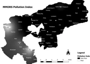
Studies focusing on water quality of water bodies from major transboundary rivers MMORS hydrographical area are scarce, so this study has great importance for the reason that it describes the suitability of surface water sources from this hydrographical area for human consumption being useful for communication of overall water quality information to the concerned citizens and policymakers. This is reflected in the spatial distribution of the overall pollution index which is illustrated in the succeeding figure. Fig. 12 merely attests that almost 80% of the sampling stations for the most part of Meycauayan and Marilao are massively polluted after undergoing test results to predict the entire MMORS condition with its corresponding water pollution level classification indicated as ‘Very Poor‘ whereas Obando river area which is nearly 20% of the remaining in the heat map is graded as ‗Poor‘.

Fig. 12. Overall pollution index spatial distribution.

IV. CONCLUSION

(7)

DENR-EMB Region 3. The resulting accuracies of the predicted model scored 99.38% in terms of correctly classified instances and are able to generate 0.8303 Kappa values which indicate that the model used, produced a strong level of agreement. Based on the heat map of the different water quality parameter and overall population index spatial distribution, majority of the sampling station are greatly polluted provided that they have ‘Poor’ and ’Very Poor’ condition as observed in the foregoing figures.

The author recommend that this study, visualizing a data-driven approach in providing pollution level estimation that is viable regardless of the water parameter of a particular river system and that the predictive modeling method, be implemented on various major river systems across the Philippines.

ACKNOWLEDGMENT

The author acknowledges DENR-EMB Region 3 for providing the historical dataset of MMORS. This study has an ongoing budget proposal to the local executive of Marilao-Meycauyan-Obando.

CONFLICT OF INTEREST The author declares no conflict of interest.

AUTHOR CONTRIBUTIONS

J,V conceived and carried out the study, wrote the paper from draft to final manuscript. A,V participated as collaborator of DENR-EMB Region 3 for providing the historical dataset of MMORS preprocessing, helped during the data mining stage, and optimized the result of algorithm used. L,L participated in the design and coordination of the study and validated the dataset and the result. All authors had approved the final version.

REFERENCES

[1] J. M. S. Amparo, M. T. M. Talavera, A. S. A. Barrion, M. E. T. Mendoza, and M. B. Dapito, ―Assessment of fish and shellfish consumption of coastal barangays along the Marilao-Meycauayan-Obando River System ( MMORS ), Philippines,‖ vol. 23, no. 2, pp. 263–277, 2017.

[2] M. C. Malenab, E. Visco, D. Geges, J. M. Amparo, D. Torio, and C. E. Jimena, ―Analysis of the integrated water resource management in a water quality management area in the Philippines : The case of Meycauayan-Marilao-Obando River System,‖ vol. 98, December, pp. 84–98, 2016.

[3] R. Paje and J. M. Cuna, ―Department of environment and natural R esources,‖ Water Quality Guidelines and General Effluent Standard of 2016, Department of Environment and Natural Resources, 2016, p. 03. [4] N. El-Jabi, D. Caissie, and N. Turkkan, ―Water quality index assessment under climate change,‖ J. Water Resour. Prot., vol. 06, no. 06, pp. 533–542, 2014.

[5] S. Yang and H. Zhang, ―Comparison of several data mining methods in credit card default prediction,‖ Intell. Inf. Manag., vol. 10, no. 05, pp. 115–122, 2018.

[6] F. C. C. Garcia, A. E. Retamar, and J. C. Javier, ―Development of a predictive model for on-demand remote river level nowcasting : Case study in Cagayan River Basin, Philippines,‖ pp. 3275–3279, 2016. [7] A. Liaw and M. Wiener, ―Classification and regression by random

forest,‖ R news, vol. 2, no. December, pp. 18–22, 2002.

[8] A. Parparov, ―Water quality assessment, trophic classification and water resources management,‖ J. Water Resour. Prot., vol. 02, no. 10, pp. 907–915, 2010.

[9] B. Abu-salih, P. Wongthongtham, K. Y. Chan, B. Abu-salih, P. Wongthongtham, and K. Y. Chan, ―Twitter mining for ontology-based domain discovery incorporating machine learning,‖ 2018.

[10] J. R. Landis and G. G. Koch, ―The measurement of observer agreement for categorical data,‖ Biometrics, vol. 33, no. 1, p. 159, 1977. [11] S. Subramani, T.; Krishnan and P. K. Kumaresan, ―Study of

groundwater quality with GIS application for Coonoor Taluk in Nilgiri district,‖ Int. J. Mod. Eng. Res., vol. 2, no. 3, pp. 586–592, 2012. [12] S. Chainey, L. Tompson, and S. Uhlig, ―The utility of hotspot mapping

for predicting,‖ pp. 4–28, 2008.

[13] Zhou-Lin. Hotspot mapping technique. [Online]. Available: https://www.semanticscholar.org/paper/A-web-based-geographical-in formation-system-for-and-Zhou-Lin/1efc5d43a95af5f9e14a8cf63bce9 b9e4853b31f/figure/0

[14] S. Chainey, ―Examining the influence of cell size and bandwidth size on kernel density estimation crime hotspot maps for predicting spatial patterns of crime,‖ BSGLg, vol. 60, no. 1, pp. 7–19, 2013.

Copyright © 2020 by the authors. This is an open access article distributed under the Creative Commons Attribution License which permits unrestricted use, distribution, and reproduction in any medium, provided the original work is properly cited (CC BY 4.0).

Jayson M. Victoriano obtained a master degree in computer science at Our Lady of Fatima University, Valenzuela City, Philippines in 2017. Currently, he is studying for the doctor degree in information technology at AMA University, Philippines as scholar of the Commission on Higher Education. He is a faculty member of Bulacan State University, Philippines. His research interest is in machine learning, data mining and AI.

Luisito L. Lacatan has a PhD in Mathematics, he is the former chairperson of the computer engineering and Coordinator of graduate school of engineering in Adamson University, Manila Philippines, currently he is the Dean of College of Engineering at AMA University, Quezon City, Philippines.