Bearing Fault Prediction using Filter Based Feature
Selection Methods and Datamining Techniques
S.Devendiran
1,N Harsha Teja
2, D N Praveen
3& C Hoshima Reddy
4 1,2,3&4School of Mechanical Engineering, VIT University, Vellore, Tamil Nadu, India [email protected] &[email protected]
Abstract– The present work proposes a vibration signal based intelligent bearing fault diagnosis using various prediction models. It includes different feature selection algorithms ReliefF, Information gain, Gini index and random forest algorithm, subsequently classifiers such as JRip,J48,Reduce error pruning, Logistic model tree (LMT) , decision table and RIDOR were used to predict the bearing conditions .The experiment were conducted for four cases such as Normal Bearing, Inner race fault, Outer race fault and Ball fault, at constant speed and load conditions and the vibration data is obtained . The aim of the paper to identify an appropriate model for that maintains high accuracy with adequate computational time. It was observed that RIDOR possess higher accuracy than other classifiers and LMT given optimum computational time with decent accuracy prediction. Other parameters related to classification process were also discussed.
IndexTerm-- Fault Diagnosis, Statistical Features, data mining techniques etc.
I. INTRODUCTION
Rolling-element bearings generally have crucial and various applications in different engineering fields. It can be proven mainly due to its load bearing capacity, low speed as well as high speed applications and anti-friction property. However, the roller bearings yield to failure due to variation in radial and axial loads and also due to wear and prolonged usage. Due to its wide scale application, it becomes mandatory to diagnose any type of fault as quick as possible within the shortest time possible so as to prevent the devastation caused due to the fault. These faults are diagnosed by ‘Bearing conditioning methods’. Conditioning methods can include information derived from physical inspection, wear properties or analysis of working parameters. [1] Furthermore, it was found that vibration analysis was the most optimum technique used for fault diagnosis as it a reliable source due to the fact that it provides real-time data over a wide range of conditions giving rise to an unbiased dataset. Adding to that, vibration analysis not only maintains correlation with the working conditions of the bearing, but also provides unique results for distinct kinds of faults. [2] The present paper contains of 4 types of signals: 1) Outer race fault; 2) Normal (no fault); 3) Ball fault; 4) Inner race fault. To make the result as comprehensive as possible numerous data are collected under each category. The real time data collection is under the time domain. Hence in order to get the Frequency domain, there is a need to perform Fast Fourier Transform (FFT) [3]. FFT is one of the most widely used signal processing techniques. However, when the frequency resolution, steady state magnitude results and comparing other data processing
Fourier Transform (STFT) is used in order to counter this drawback. In STFT, the signal is processed by combining data from the frequency domain as well as time. This enables a crystal clear picture of when and at what frequencies a signal occurs. The variable for STFT is the size of the window used; this could also be considered as a drawback resulting in lesser precision. [4] Depending on the frequency Wavelet transformation (WT) is a more refined signal processing technique that discretizes the signal into wavelets [5]. WT acquires data from both the frequency and time domain and hence can extract transitory features [6]. WT is categorized into Continuous Wavelet Transformation (CWT) and Discrete wavelet transformation (DWT) [7]. Statistical feature reduction is the next step that follows signal processing. Statistical parameters like kurtosis, standard deviation, skewness, mean, variance, maximum, minimum, median, mean slope, maximum slope and minimum slope were calculated for time domain as well as frequency domain, from the dataset. One such technique is Principal component analysis (PCA). As we can describe PCA as widely used method for data mining and data recollection applications. It transforms a set of correlated variables into a set of linearly uncorrelated variables.
classification algorithms.[13] applied automatic rule learning using decision tree for fuzzy classifier in fault diagnosis of roller bearing, a rule set is formed from the extracted features and input to a fuzzy classifier. Decision tree is used to generate the rules automatically from the feature set. [14] Utilized genetic algorithm for optimal feature selection in mechanical fault detection of induction motor. Based on specific distance criteria, a Genetic Algorithm (GA) is introduced to reduce the number of features. A decision tree and multi-class support vector machine are used to illustrate the potentiality and efficiency of this selection (classification)
method. [15] Suggested some methods to extract features using envelope analysis accompanied by Hilbert Transform and Fast Fourier Transform. The proposed ANN based fault estimation algorithm was verified with experimental tests and ANN model was modified using a genetic algorithm providing, optimal skilful fast-reacting network architecture with improved classification results. [16] Made a Comparison of neural networks and support vector machines in condition monitoring application. . The flow chart of the diagnostic
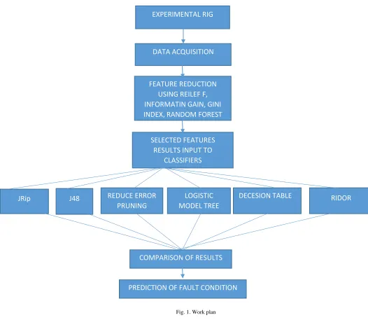
method is depicted in Fig. 1.
Fig. 1. Work plan
EXPERIMENTAL RIG
REDUCE ERROR
PRUNING
J48
JRip
FEATURE REDUCTION
USING REILEF F,
INFORMATIN GAIN, GINI
INDEX, RANDOM FOREST
DATA ACQUISITION
PREDICTION OF FAULT CONDITION
COMPARISON OF RESULTS
LOGISTIC
MODEL TREE
SELECTED FEATURES
RESULTS INPUT TO
CLASSIFIERS
II. EXPERIMENTAL SETUP
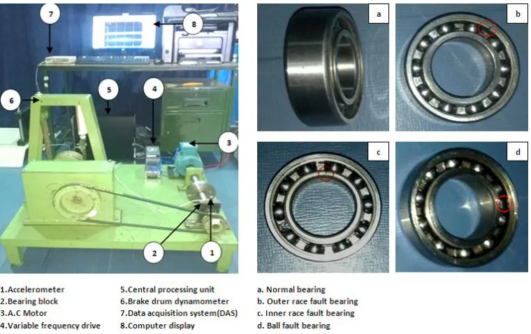
The proposed methodology is verified by performing tests on the designed experimental setup. The experimental set-up shown in Fig-1, comprises of components such as variable frequency drive (VFD), three phase 0.5 hp AC motor, bearing, belt drive, gearbox and brake drum dynamometer with scale. The present experiment utilizes a standard deep groove ball bearing (No. 6005). Measurements of the vibration acceleration signals are captured by a Triaxle type accelerometer (Vibration sensor) that is fixed over the bearing block. 24 Bit, ATA0824DAQ51 data acquisition system was used and the signals were collected at a sampling frequency of
12800 Hz. The bearing was maintained at a constant rotation and dynamometer applied a constant load and a tachometer was placed to monitor the constant speed. Fig-2 indicates normal, outer race, inner race and ball fault (1mm crack depth) conditions were formed using the EDM process. Table 1 depicts the number of sample data collected for each bearing condition. Each sample contains 6000 data points. The various conditions of bearing component using time domain and frequency domain by varying amplitudes was found out by analysing the signals. Time domain plots are illustrated in Fig.3.The frequency of the abnormal vibration is called fault frequency which corresponds to the fault location
Fig. 2. Experimental Setup
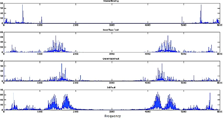
The following equations gives a detailed preview of fault characteristic frequencies for different parts of the bearing. The characteristic bearing frequencies are BPFO- Ball Pass Frequency Outer Race, BPFI- Ball Pass Frequency Inner Race, FTF- Fundamental Train Frequency and BSF- Ball Spin Frequency. Frequency analysis is considered as One of the most basic approach for bearing conditioning monitoring. Fast Fourier transform (FFT), is used to transform the time series data to frequency domain, where the signal is used to deduce the sine and cosine waves from the sample. When practically, analysing those frequencies and measuring the amplitude variations in the particular frequency and its side bands as well the harmonics of those frequencies will provide information regarding the health of the bearing. The bearing conditions are difficult to be differentiated by their FFT spectral shown in Fig.4.
Shaft rotational frequency- Fs( Hz) = Shaft
speed/60 (1)
Ball passing frequency outer race,
(BPFO)
=
(2)
Ball passing frequency inner race
(BPFI)
=
(3)
Fundamental train frequency
(FTF)
=
(4)
Ball spin frequency
1
cos
2
b d
d
N
B
Fs
P
1
cos
2
b d
d
N
B
Fs
P
1
1
cos
2
d
d
B
Fs
P
(BSF)
=
(5)
Fig. 3. Time domain signals of various states of bearing(X axis–data points, Y axis-Amplitude in ‘g’)
Fig. 4. Frequency spectrum of various states of bearing (X axis–Frequency, Y axis-Amplitude in ‘g’) 2
2 2
1
cos
2
d d
d d
P
B
Fs
B
P
After FFT, by analysing the abnormal frequency-domain amplitude the bearing can be diagnosed. After plotting time domain and frequency domain, using WPT the signals are decomposed. The decomposed signals are then processed and
the statistical features are derived using Table 1. Statistical features are extracted for both time domain as well as frequency domain and then given for feature reduction and other processes
TABLE I Statistical features
The experimental procedure is conducted by collecting data from the vibration of a motor under various fault conditions. Thus a signal is obtained for each condition of the bearing such as normal, IR fault, OR fault, and ball fault. Each signal is originally obtained in the time domain. Therefore, to obtain the frequency domain a discrete Fourier transform is applied to the signals. Statistical feature extraction each signal is broken into sub signals by considering a subset of the original number of data points. For this purpose, a total of 40 sub signals is obtained for each signal. For each sub signal, the statistical features like local mean, standard deviation, etc. are considered thus obtaining 40 data points for each signal and for each feature.
Once the data is collected, statistical features are extracted .The data signal obtained is expressed in time domain and frequency domain. 11 statistical features as explained for each domain in the previous section, which sum up to 22 statistical features. The features selected are optimized and scrutinized through feature selection methods. Along with the original unreduced feature set a total of 9 feature sets are obtained for comparison. The accuracy of classifiers were computed and the computation time is also calculated. From the results obtained, the best classification algorithm and feature selection method is determined.
Time domain feature parameters
Frequency domain feature parameters
No. Feature Equation No. Feature Equation
1 Mean
X
= N1
N t
t
x
1)
(
12 Mean_
s
=K1
K k
k
s
1)
(
2 Variance XV = N1
_ 2 1
( ( )
)
N tx t
x
13 Variance sv = K1_ 2 1
( ( )
)
K ks k
s
3 Square mean
root Xr = (N
1 1 2
2 1
)
N tx
14 Square meanroot Sr = (K
1 1 2
2
)
Kk
s
4 Root mean
square
Xrms = (
N
1
1 2 2 1)
N tx
15 Root meansquare
Srms = (
k
1
1 2 2 1( )
K ks
5 Peak - Peak
x
= E{max( x(t) )} 16 Peak - Peaks
= E{max( s(k) )}6 Skewness Xske =
_ 3 1
1
( ( )
)
N tx t
x
N
17 Skewness Sske =_ 3 1
1
( ( )
)
k ks k
s
k
7 Kurtosis Xkur =
N
1
_ 41
( ( )
)
N
t
x t
x
18 Kurtosis Skur =k
1
_ 41
( ( )
)
k
k
s k
s
8 S factor S = xrms/
x
_ 19 S factor S = srms/_
s
9 C factor C =
x
/ xrms 20 C factor C =s
/ srms10 L factor L =
x
/ xr 21 L factor L = s
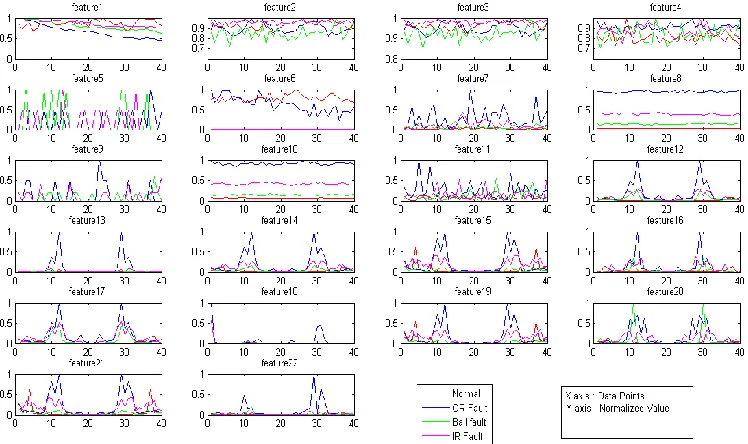
/ srFig. 5. Graphical representation of features selected for each fault case
Feature 1 to 11 are in the time domain and features 12 to 22 are in the frequency domain. It is advantageous to analyse statistical features in the frequency domain as well because cases with faults show different frequency peaks and peaks which are higher than that without a fault. The unreduced feature set of the original 22 features is considered as well and therefore there are 9 total feature sets taken into consideration. The computation time for each feature selection algorithm is calculated. D. Classification process the classification accuracy is computed for each feature set using different classifiers and neural nets. For this purpose, Random Forest (RF), Reduce Error Pruning (REP) and Logistic Model Tree (LMT) and J48 algorithms are used. The classification accuracy and computation time for each classifier are calculated.
III. THEORETICAL BACKGROUND OF FEATURE
SELECTION ALGORITHMS
This part of this paper briefly introduces the feature selection algorithms that has been discovered and reported in the literatures. The feature selection algorithms are classified into three categories such as filter model, wrapper model and embedded model according to the computational models. The filter model relies on the general characteristics of data and evaluates features without involving any learning algorithm. The wrapper model requires having a predetermined learning algorithm and uses its performance as evaluation criterion to select features. The embedded model incorporate variable selection as a part of the training process, and feature relevance is obtained analytically from the objective of the learning model.
A.ReliefF (RF)
ReliefF [17] is a supervised multivariate feature selection algorithm of the filter model which is the extension of Relief is a univariate model. Assuming that p instances are randomly sampled from data, the evaluation criterion for handling multiclass problems is of the form
SC
R(f
i) =
p
1
.
p
t 1
{
-mxt
1
) (Xt NM xjd
(f
t,i– f
j,i) +
yxt y
mxt
,
y
1
)
(
1
)
(
yxt
p
y
p
XNM
(Xt,y)d
(f
t,i– f
j,i)} (6)
where yxt is the class label of the instance xt and P(y) is the probability of an instance being from the class y. NH(x) or NM(x, y) denotes a set of nearest points to x with the same class of x, or a different class (the class y), respectively. Mxt and Mxt, y are the sizes of the sets NH (xt) and NM(xt, y), respectively. Usually, the size of both NH(x) and NM(x, y); ¥ y ≠ yxt , is set to a pre-specified constant k.
B. Information Gain (IG)
Information Gain [18] is supervised univariate feature selection algorithm of the filter model which is a measure of dependence between the feature and the class label. It is one of the most powerful feature selection techniques and it is easy to compute and simple to interpret. Information Gain (IG) of a feature X and the class labels Y is calculated as
)
/
(
)
(
)
,
(
X
Y
H
X
H
X
Y
Entropy (H) is a measure of the uncertainty associated with a random variable. H(X) and H(X/Y) is the entropy of X and the entropy of X after observing Y, respectively.
H(X)
= -
i
P
(X
i) log
2(P(X
i))
(8)
The maximum value of information gain is 1. A feature with a high information gain is relevant. Information gain is evaluated independently for each feature and the features with the top-k values are selected as the relevant features. This feature selection algorithm does not eliminate redundant features.
H(x/y) = -
jP
(Y
j)
iP
(X
i/Y
j) log
2(P (x
i/y
j))
(9)
C. Gain Ratio
The most prominent drawback of information gain measure is that this methodology works towards tests with many outcomes. That is, it prefers to select attributes having a large number of possible values over features with fewer values even though the latter is more informative. For example consider an attribute that acts as a unique identifier, such as an employee Number in the employee database. A split on this feature would result in a large number of partitions; as each record in the database has a unique value for employee number. So the information required to classify database with this partitioning would be 0. Clearly, such a partition is useless for classification.
Let D be a set consisting of d data samples with n distinct classes. The expected information needed to classify a given sample is given by
I(D)=−Σpini=1log2( pi)
(10)
Where pi is the probability that an arbitrary sample belongs to class Ci. Let attribute A have v distinct values. Let dijbe number of samples of class Ci in a subsetDj. Dj Contains those samples in D that have value aj of A. The entropy based on partitioning into subsets by A
A, is given by
E(A)=−ΣI(D)( d1i+d2i+⋯ dmi)dni=1
(11) The encoding information that would be gained by branching on A is
Gain (A)=I(D)−E(A)
(12)
C4.5 applies a kind of normalization to information gain using a “split information” value defined analogously with Info (D) as
Split InfoA(D)−ΣDj|D|vj=i log2(|Dj||D|)
(13) This value represents the information computed by splitting the dataset D, into partitions, corresponding to the v outcomes
of a test on feature A. For each possible outcome, it considers the number of tuples having that outcome with respect to the total number of tuples in D. The gain ratio is defined as
𝐺𝑎𝑖𝑛 (𝐴)=Gain (A)SpiltInfo(A)
(14)
The attribute with maximum gain ratio is selected as the splitting attribute.
GR =
)
(
X
H
IG
(15)
D. Gini Index (GI)
Gini index [19] is supervised multivariate feature selection algorithm of the filter model to measure for quantifying a feature's ability to distinguish between classes. Given C classes, Gini Index of a feature f can be calculated as Gini Index can take the maximum value of 0.5 for a binary classification. The more relevant features have smaller Gini index values. Gini Index of each feature is calculated independently and the top k features with the smallest Gini index are selected. Like Information gain, it also not eliminates redundant features.
Gini Index (f) = 1 -
C
i
f
i
P
1
2
)]^
/
(
[
(16)
E. Random Forest (RF)
Random Forest algorithm was initially developed by Leo Breiman, [20] a statistician at the University of California Berkeley [24]. Random features are selected using the induction process. Prediction is made by aggregating the predictions of the ensemble. Random Forest generally proves a significant performance improvement as compared to single tree classifier C4.5.Random Forests is a method by which one can calculate accuracy rate in better way. Some attributes of Random Forest is mentioned below.
[1]. It efficiently works on large data sets (training data sets).
[2]. It provides consistent accuracy than the other algorithms.
[3]. by this method estimate missing data if any and retains the accuracy rate even if the bulk of the data is missing.
[4]. It also provides an estimate of important attributes in the classification.
The strength of RF is mentioned below
1) RF may produce a highly accurate classifier for more data sets.
2) RF has much simplicity.
III. THEORETICAL BACKGROUND OF CLASSIFIERS. Classification of data is the segregation of data based on certain decided attributes and qualities. Data mining essentially classifies the useful data into a sub population and separates them from the entire data set. Classifier is an algorithm that carries out this classification process. The term classifier at times is also referred as a mathematical function that processes the data fed in and outputs data that is distinctly categorised. Different classifiers have different algorithms, each having its own parameters such as computing time and efficiency. In the present paper, several classifiers have been used and compared their results with each other in order to check the best amongst them. Classification techniques can be compared on the basis of predictive accuracy, speed, robustness, scalability and interpretability criteria [21]. In data mining classification tree is a supervised learning algorithm. So one can prepare popular classifiers: J48, Random Forest, Reduce Error Pruning, Logistic Model Tree, JRip, RIDOR and Decision Table.
A. JRIP
JRIP implements a propositional rule learner. William W. JRip proposed a Repeated Incremental pruning to produce Error Reduction (RIPPER). It is an inference and rules-based learner (RIPPER) that can be used to classify elements with propositional rules. The RIPPER algorithm is a direct method used to extract the rules directly from the data. The algorithm progresses through four phases: i) growth, ii) pruning, iii) optimization and iv) selection [30] [31].
B. J48 Algorithm
J48 is a tree based learning approach. It is developed by Ross Quinlan which is based on iterative dichotomise (ID3) algorithm [23] J48 uses divide-and-conquer algorithm to split a root node into a subset of two partitions till leaf node (target node) occur in tree. Given a set T of total instances the following steps are used to construct the tree structure.
Step 1: If all the instances in T belong to the same group class or T is having fewer instances, than the tree is leaf labelled with the most frequent class in T.
Step 2: If step 1 does not occur then select a test based on a single attribute with at least two or greater possible outcomes. Then consider this test as a root node of the tree with one branch of each outcome of the test, partition T into corresponding T1, T2, T3..., according to the result for each respective cases, and the same may be applied in recursive way to each sub node.
Step 3: Information gain and default gain ratio are ranked using two heuristic criteria by algorithm J48.
C. Reduce Error Prune
This method introduced by Quinlan [25]. It is the simplest and most understandable method in decision tree pruning. For every non-leaf sub tree of the original decision tree, the
change in misclassification over the test set is examined. The REP incremental pruning developed by Written and Frank in 1999 is a fast regression tree learner that uses information variance reduction in the data set which is divided into a training set and a prune set. When any one traverse the tree from bottom to top then he she may apply the procedure which checks for each internal node and replace it with most frequently class, keeping in mind about tree accuracy, which must not reduce. Now the node is pruned. This procedure will continue until any further pruning would decrease the accuracy.
D. Logistic Model Tree
Logistic Model Tree (LMT) [26] algorithm makes a tree with binary and multiclass target variables, numeric and missing values. So this technique uses logistic regression tree. LMT produces a single outcome in the form of tree containing binary splits on numeric attributes.
E. DECISION TABLE
A decision table specifies only the logical rules. It is used to find out the decision quality. Conditional logic in this context refers to a set of tests, and a set of actions to take as a result of these tests. The classifier rules decision table is described as building and using a simple decision table majority classifier. The decision table classifiers has two variants such as o DTMaj (Decision Table Majority) or DTLoc(Decision Table Local) Decision Table Majority returns the majority of the training set if the decision table cell matching the new instance is empty, that is, it does not contain any training instances. Decision Table Local is a new variant that searches for a decision table entry with fewer matching attributes (larger cells) if the matching cell is empty. Hence this variant returns an answer from the native region [32] [33].
F. RIDOR
Ripple down Rule learner (RIDOR) is also a direct classification method. It constructs the default rule. An incremental reduced error pruning is used to find exceptions with the smallest error rate, finding the best exceptions for each exception, and iterating. The most excellent exceptions are created by each exceptions produces the tree-like expansion of exceptions. The exceptions are a set of rules that predict classes other than the default. IREP is used to create exceptions [29].
VI. EXPERIMENTAL RESULTS
into two types: Time and frequency domain features that are extracted from Time and frequency and selected features from the same are separately fed input into WEKA embedded classifiers such as JRIP, J48, REDUCE ERROR PRUNE, LOGISTIC MODEL TREE, DECISION TABLE and RIDOR to identify different states of gear through classification process. To measure and investigate the performance of the classification algorithms 75% data is used for training and the remaining 25% for testing purpose. The results of the simulation are shown in Tables 4 and 5. Table 4 summarizes the results based on accuracy and time taken for each simulation. Meanwhile, Table 5 shows the results based on error during the simulation. Figures- 8 and 9 shows the graphical representations of the simulation results. Based on the result (Table 4.) it can be clearly noted that the highest accuracy is 93.4 % and the lowest is 72.2%. The results are discussed based on various performance parameters and it is explain detailed in [28].
A. Cost Matrix
A cost matrix is similar to confusion matrix but minor difference is with finding the value of cost accuracy through misclassification error rate
.
Misclassification error rate = 1 – Accuracy
B. Calculate Value TPR, TNR, FPR, and FNR One can calculate the value of true positive rate, true negative Rate, false positive rate and false negative rate by methods Shown below.
TPR=
FN
TP
TP
(18)
TNR=
TN
FP
TN
(19)
FPR=
FN
TP
FN
(20)
FNR=
TN
FP
FP
(21)
C. Recall
Recall is the ratio of modules correctly classified as fault-Prone to the number of entire faulty modules.
Recall =
FP
TN
TP
(22) D. Precision
Precision is the ratio of modules correctly classified to the Number of entire modules classified fault-prone. It is Proportion of units correctly predicted as faulty.
Precision =
FP
TP
TP
(23)
E. F-Measure
FM is a combination of recall and precision. It is also defined As harmonic mean of precision and recall.
F-Measure =
PRECISION
RECALL
PRECISION
RECALL
2
(24)
F.Accuracy
It is defined as the ratio of correctly classified instances to total number of instances.
Accuracy =
FN
TN
FP
TP
TN
TP
Fig. 6. Top 10 predominant features with its ranking value
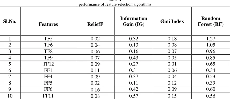
Table II
performance of feature selection algorithms
Sl.No.
Features ReliefF
Information
Gain (IG) Gini Index
Random Forest (RF)
1 TF5 0.02 0.32 0.18 1.27
2 TF6 0.04 0.13 0.08 1.05
3 TF8 0.06 0.16 0.07 0.96
4 TF9 0.07 0.43 0.05 0.85
5 TF12 0.09 0.27 0.01 0.65
6 FF1 0.11 0.31 0.06 0.34
7 FF4 0.09 0.37 0.04 0.53
8 FF5 0.02 0.11 0.12 0.39
9 FF6 0.16 0.42 0.09 0.60
10 FF11 0.08 0.57 0.15 0.56
This work also observes that Random forest outperforms than all other feature selection algorithms, IG and GR are the next better feature selection algorithms. Result and the ReliefF
gave equally poor performance in feature selection and ranking. The performance of all 4 filter based feature selection algorithms is depicted in Figure 6 and Table 2 respectively.
Table III
Prediction Performance Measures
Classifier TPR FPR TNR FNR Precision Recall F-measure Accuracy in
%
Total Time Taken (sec)
JRip 0.82 0.64 0.57 0.88 0.90 0.88 0.91 92.45 0.021
J48 0.87 0.73 0.69 0.79 0.82 0.80 0.85 89.35 0.026
REP 0.82 0.92 0.87 0.75 0.85 0.83 0.88 87.72 0.091
LMT 0.90 1 0.91 0.83 0.90 0.92 0.92 93.23 0.157
Decision table
0.90 0.88 0.66 0.87 0.90 0.95 0.90 91.87 0.011
RIDOR 0.91 0.90 0.89 0.76 0.92 0.92 0.95 97.60 0.019
0 0.2 0.4 0.6 0.8 1 1.2 1.4
TF5 TF6 TF8 TF9 TF12 FF1 FF4 FF5 FF6 FF11
Ran
kin
g v
alu
e
Features
Features
ReliefF (RF)
Information Gain (IG)
Gini Index
Table IV Error rate measurement
Classifier MSE RMSE RAE RSE
JRip 0.04 0.20 12.98 45.65
J48 0.05 0.21 14.80 48.23
REP 0.03 0.20 12.02 44.94
LMT 0.05 0.22 14.95 47.12
Decision table 0.09 0.29 22.56 60.29
RIDOR 0.02 0.18 11.12 41.22
V. RESULTS AND DISCUSSION
The bearing fault prediction is majorly based on classification accuracy and it is depicted in Table 3 show that the accuracies are different, although the selected sensitive features are the same, also with different classifiers. Therefore, the feature and classifier should be studied as a whole. The results from the analysis of the selected sensitive features indicate that no statistical feature achieved a favourable classification performance in all of the fault datasets. This phenomenon reveals that each statistical feature plays multiple roles in different fault diagnoses. Thus, diagnosis can be made after adaptive selection of sensitive fault features according to different fault types. In Fig. 6 comparison made with the top ten predominant feature with its ranking value, by which it can be conclude that Random Forest (RF) gives the highest ranking when its predominant feature values are compared with other feature selection methods .In fig7 we have plotted a graph between TPR, FPR, TNR, FNR, Precision, Recall, F-Measure and classifiers with the help of obtained results. From the graphs the following can be concluded that the TPR value is higher for RIDOR classifier, FPR value is higher for LMT classifier, TNR value is higher for RIDOR classifier, FNR value is higher for JRip classifier, Precision value is higher for
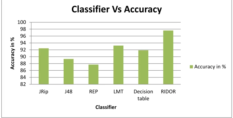
RIDOR classifier, Recall value is higher for RIDOR classifier and F-measure is higher for RIDOR classifier. Whereas from table 3 we have found that accuracy of RIDOR is 97.6% which can be deduced as best among JRip, J48, REP, LMT and Decision table methods of classification. Similarly Figure 9 depicts that the total time taken by LMT is 0.157 which is higher when compared to other classifiers. In fig 10 and fig 11 the comparison of error rate measure for the rule classifier algorithms such as JRip, J48, REP, LMT, Decision Table, and RIDOR has been plotted. From the results, RIDOR produces the lower error rate when compared to other classifiers. Where, in fig 10 MSE value and RMSE value is higher for Decision table classifier and in fig 11 RAE value and RSE value is higher for decision table classifier. Cross-validation (CV) method used in order to validate the predicted model. CV test basically divide the training data into a number of partitions or folds. The classifier is evaluated by accuracy on one phase after learned from other one. This process is repeated until all partitions have been used for evaluate the most common types are 10-fold, n-fold and bootstrap result obtained into a single estimation.
Fig. 7. Classifier Vs Performance Measures
0 0.2 0.4 0.6 0.8 1 1.2
JRip J48 REP LMT Decision table
RIDOR
Per
for
m
an
ce
M
e
asu
re
s
Classifier
Classifier Vs Performance Measures
Fig. 8. Classifier Vs Accuracy
Fig. 9. Classifier Vs Total Time Taken
82 84 86 88 90 92 94 96 98 100
JRip J48 REP LMT Decision table
RIDOR
A
cc
u
rac
y in
%
Classifier
Classifier Vs Accuracy
Accuracy in %
0 0.02 0.04 0.06 0.08 0.1 0.12 0.14 0.16 0.18
JRip J48 REP LMT Decision table
RIDOR
To
tal Ti
m
e
Take
n
in
Sec
Classifier
Classifier Vs Total Time Taken
Fig. 10.(Classifier Vs Mean square error)
Fig. 11.
Classifier Vs Error
VI. CONCLUSIONS
A new intelligent diagnosis approach is presented in this study for the purpose of improving the diagnostic accuracy of rolling bearing compound faults. Statistical features of vibration signal contain abundant fault information; thus, the selection of 22 statistical feathers in the time and frequency domains were initially undertaken. Meanwhile, in order to remove the redundant and irrelevant information features INFORMATION GAIN, GINI INDEX, GAIN RATIO and RELIEF-F is implemented and the algorithm showed promising results in optimized feature selection process as well in prediction results. To compare the success rates, classification metrics such as JRIP, J48, REDUCE ERROR PRUNE, LOGISTIC MODEL TREE, DECISION TABLE and RIDOR are performed without feature selection and after
feature selection process. Altogether, extracted features optimized by Random forest and Ridor give a better result based on classification accuracy when compared to other schemes in the same condition in bearing fault diagnosis.
REFERENCE
[1] HocineBendjama, Salah bouhouche, Mohamed SeghirBoucherit, “Application of wavelet transform for fault diagnosis in rotating machinery”, International Journal of machine learning and Computing, Vol.2, No.1 , Feb 2012
[2] SaravanaBharathi K, Shajeev M, Nair Pravin R, Prasath Kumar P, Santhosh kumar C, “Application of Multi-Wavelet Denoising and Support Vector Classifier in Induction Motor Fault Conditioning”, International Journal of Computer Applications, Vol.8, Article 1, 2011
0 0.05 0.1 0.15 0.2 0.25 0.3 0.35
JRip J48 REP LMT Decision table
RIDOR
Er
ror
Rate
M
easur
e
Classifier
Classifier Vs Error Rate Measure
MSE RMSE
0 10 20 30 40 50 60 70
JRip J48 REP LMT Decision table
RIDOR
Er
ro
r
R
ate
M
e
asu
re
Classifier
Classifier Vs Error
[3] Milind Natu, “Bearing Fault Analysis Using Frequency Analysis and Wavelet Analysis”, International Journal of Innovation, Management and Technology, Vol. 4, No. 1, February 2013 [4] NeelamMehala, RatnaDahiya, “Condition monitoring methods,
failure identification and analysis for Induction machines”, International journal of circuits, systems and signal processing, Issue 1, Vol. 3, 2009
[5] KhalafSalloumGaeid and Hew WooiPing, “Wavelet Fault Diagnosis of Induction Motor” , MATAB for Engineers- Applications in Control , Electrical Engineering, IT and Robotics, Oct 2011
[6] Hui lui, Lihui Fu, Haiqi Zheng, “Bearing Fault diagnosis based on amplitude and phase map of Hermitian wavelet transform” , Journal of Mechanical Science and Technology, Vol. 25, Issue 11, P 2731-2740, Nov 2011
[7] N.S. Swansson and S.C Favaloro, “Applications of vibration analysis to the condition monitoring of rolling element bearings”, Defence science and technology organisation, Aeronautical research laboratories, Melbourne, Aero propulsion report 163, January 1984
[8] Lei, Y., Z. He., Y. Zi., and Q. Hu Fault diagnosis of rotating machinery based on multiple ANFIS combination with GAs. Mechanical Systems and Signal Processing, Vol. 21, No. 5, pp. 2280-2294. 2007.
[9] Matsuura, T An Application of Neural Network for Selecting Feature Parameters in Machinery Diagnosis, Journal of Materials Processing Technology, Vol. 157-158, pp. 203–207. 2004. [10] Saravanan, N., S. Cholairajan and K. I. Ramachandran
Vibration-based fault diagnosis of spur bevel gear box using fuzzy technique, Expert systems with applications, Vol. 36, No. 2, pp. 3119-3135. 2009.
[11] Baillie D.C. and J. MathewA comparison of autoregressive modeling techniques for fault diagnosis of roller element bearings, Mechanical Systems and Signal Processing, Vol. 10, pp. 1-17. 1996.
[12] Liu T.I., Singonahalli J.H., and Iyer N.R Detection of Roller bearing defects using expert system and fuzzy logic, Mechanical Systems and Signal Processing , Vol. 10,pp. 595-614. 1996. [13] Sugumaran,V and K. I. Ramachandran Automatic rule learning
using decision tree for fuzzy classifier in fault diagnosis of roller bearing, Mechanical Systems and Signal Processing, Vol. 21, pp. 2237-2247. 2007.
[14] Ngoc-Tu Nguyen, Hong-Hee Lee and Jeong-Min Kwon Optimal feature selection using genetic algorithm for mechanical fault detection of induction motor, Journal of Mechanical Science and Technology, Vol. 22 , pp. 490~496. 2008.
[15] Dalpiaz , G., A. Rivola and R. Rubini Effectiveness and sensitivity of vibration processing techniques for local fault detection in gears. Mechanical System and Signal Processing, Vol. 14, No. 3, pp. 387-412. 2000.
[16] Unal., M. Onat., M. Demetgul and H. Kucuk Fault diagnosis of rolling bearings using a genetic algorithm optimized neural network, Measurement, Vol. 58, pp. 187-196. 2014.
[17] [Hall, M.A., and Smith, L.A., “Practical feature subset selection for machine learning”, Proceedings of the 21st Australian Computer Science Conference, 1998, 181–191.]
[18] M.A. Hall. Correlation-based feature selection for discrete and numeric class machine learning. In Proceedings of the Seventeenth International Conference on Machine Learning, pages 359–366, 2000]
[19] George Forman. An extensive empirical study of feature selection metrics for text classi_cation. Journal of Machine Learning Research, 3:1289-1305, 2003
[20] P. Langley. Selection of relevant features in machine learning. In Proceedings of the AAAI Fall Symposium on Relevance, pages 140–144, 1994
[21] J. Han and M. Kamber, “Data Mining: Concept and Techniques”, Morgan Kaufmann Publishers, 2004.
[22] J. Han and M. Kamber, “Data Mining: Concept and Techniques”, Morgan Kaufmann Publishers, 2004][9][ J.R. Quinlan, “Induction of Decession Trees : Machine Learning”,vol.1,pp.81-106,1986.
[23] J. R. Quinlan, “C4.5: Programs for Machine Learning”, San Mateo,CA, Morgan Kaufmann Publishers,1993.
[24] L. Breiman, “Random Forests. Machine Learning,” vol.45(1), pp. 5-32, 2001
[25] J.R. Quinlan, “Simplifying decision trees”, Internal Journal of Human Computer Studies,Vol.51, pp. 497491, 1999
[26] N. Landwehr, M. Hall, and E. Frank, “ Logistic model trees”. for Machine Learning.,Vol. 59(1-2),pp.161-205, 2005.
[27] N. Laves son and P. Davidson, “Multi-dimensional measures function for classifier performance”, 2nd. IEEE International conference on intelligent system, pp.508-513, 2004.
[28] Performance Analysis of Classification Tree Learning Algorithms D. L. Gupta A. K. Malviya& Satyendra Singh October 2012 [29] Gaines, B.R., Paul Compton, J. 1995. Induction of Ripple-Down
Rules Applied to Modeling Large Databases, Intell. Inf. Syst. 5(3):211-228.
[30] C. Lakshmi Devasena, T. Sumathi, V.V. Gomathi and M. Hemalatha,” Effectiveness Evaluation of Rule Based Classifiers for the Classification of Iris Data Set”, Bonfring International Journal of Man Machine Interface, Vol. 1, Special Issue, December 2011
[31] M. Thangaraj, C.R.Vijayalakshmi. Performance Study on Rule based Classification Techniques across Multiple Database Relations. International Journal of Applied Information Systems (IJAIS), Foundation of Computer Science FCS, New York, USA Volume 5– No.4, March 2013.
[32] Petra Kralj Novak, “Classification in WEKA”.