1112701-4646 IJBAS-IJENS © February 2011 IJENS
Perturbation Technique for Analytical Solution of
Fourth Order Near Critically Damped Nonlinear
Systems
Md. Asraful Alom
1, Md. Habibur Rahman
2, B. M. Ikramul Haque
3and M. Ali Akbar
4 1,2,3Department of Mathematics, Khulna University of Engineering & Technology , Khulna-9203, Banladesh4
Department of Applied Mathematics, University of Rajshahi, Rajshahi-6205, Bangladesh Abstract-- A technique is developed in this article based on
the Krylov-Bogoliubov-Mitroplskii method to investigate the solution of fourth order near critically nonlinear system in the case of
3
3
1 and
4
3. The method is illustrated by an example and the solutions obtained by this method agree nicely with those obtained by numerical method.I. INT RODUCT ION
First the Krylov-Bogoliulov-Mitropolskii (KBM) [8, 9] method was developed to find periodic solutions of second order nonlinear differential equations with small nonlinearities. Later, the method was extended by Popov [14] to damped oscillatory systems. Some meritful works and elaborative uses have been made by Minorsky [10], Bellman [7] and Nayfeh [13]. Murty and Deekshatulu [11] extended the method to nonlinear over-damped systems. Alam [4] has developed a new perturbation technique to find approximate analytical solution of second order both over-damed and critically damed nonlinear systems. Alam and Sattar [3] extended the KBM method for third order critically damped nonlinear systems. Alam [5] also investigated the solution of third order nonlinear systems when two of the eigenvalues are almost equal and the other is small. Alam [6] has presented an asymptotic method for certain third order non-oscillatory nonlinear system, which gives desired results when the damping force is near to the critical damping force. Akbar et al. [1] presented an asymptotic method for fourth order over-damped nonlinear systems, which is easier than the method presented by Murty et al. [12]. Akbar et al. [2] also extended the KBM method for solving fourth order more critically damped nonlinear systems. Recently, Rahman et al. [15] developed a technique for solving of fourth order near critically damped nonlinear systems.
For the relation
3
3
1, the solution obtained in Rahman et al. [15] break-down. In this article the aim is to investigate the solution when the above relation
3
3
1 existsamong the eigenvalues
1,
2,
3,
4 The results obtained by this method agree nicely with the numerical results.II. THE MET HOD
Let us consider the fourth order weakly nonlinear ordinary differential systems
)
(
4 3
2 2
2 3 3
1 4 4
x
f
x
c
dt
dx
c
dt
x
d
c
dt
x
d
c
dt
x
d
(1) where
is a positive small parameter,f
(
x
)
is the given nonlinear function andc
1,c
2,c
3,c
4 are constants, defined in terms of the eigen-values
λ
i,i
1
,
2
,
3
,
4
of the unperturbed equation of (1) as,
,
4
1 , 2 4
1
1 j
j i
j i
i i
i
c
c
j kk j i
k j i
i
c
41 , ,
3 and
4
1
4
λ
i i
c
.When
0
, the equation (1) becomes linear and suppose the eigenvalues
λ
1 and
λ
2 are almost equal (
1
2) and other two eigenvalues
λ
3 and
λ
4 are distinct. Therefore, the unperturbed solution is)
2
(
,
)
(
2
1
)
0
,
(
4 3
2 1 2
1
0 , 4 0
, 3
2 1 0 , 2 0
, 1
t t
t t
t t
e
a
e
a
e
e
a
e
e
a
t
x
where
a
i,0(
i
1
,
2
,
3
,
4
)
are arbitrary constants. When
0
, following Alam’s [5-6] technique we choose the solution of (1) in the form)
3
(
)
,
,
,
,
(
)
(
)
(
)
(
)
(
)
(
2
1
)
,
(
2 4
3 2 1 1
4 3
2 1
2 1
4 3
2 1
2 1
t
a
a
a
a
u
e
t
a
e
t
a
e
e
t
a
e
e
t
a
t
x
t t
t t
t t
where
a
i(
i
1
,
2
,
3
,
4
)
satisfy the first order differential equation
2 4
3 2 1
1
(
,
,
,
,
)
)
(
A
a
a
a
a
t
dt
t
da
i, (4) Confining only to a first few terms
1
,
2
,
3
,
,
n
in theseries expansions (3) and (4), we calculate the functions
u
1and
A
i,
i
1
,
2
,
3
,
4
such that ai(t), i1, 2, 3,4appearing in (3) and (4) satisfy the given differential equation (1) with an accuracy of order
n1. To determine the unknown functionsu
1,
A
1,
A
2,
A
3,
A
4 it is assumed (as customary in the KBM method) that the correction term,u
1 does not contain secular-type termt
e
it, which make them large. Differentiating equation (3) four times with respect t, substituting the derivativesdt
dx
dt
x
d
dt
x
d
dt
x
d
,
,
,
22
3 3
4 4
and
x
in the original equation (1), utilizing the relations presented in (4) and finally equating the coefficients ofε
yields,) 5 ( )
)( )(
)( (
2 2 )
(
) )(
)( (
) )(
)( (
) 2 3 (
) 2 3 (
) (
) )(
)( (
) )(
)( (
2 1
) 0 ( 1 4 3
2 1
2 1 3 2
1 2 1
2 1 3 4
2 1
4 3 4 2
4 1
4
3 4 3 2
3 1
3 2
3 2 3
1 4
1 4 2 3
2 1
2
4 1 3
1 2 1
2 1
2 1 4
3
2 1
2 1
f u D D
D D
A D
D e e
A D
D D e e
A D
D D
e
A D
D D
e A
D e
D e
D
A D
D D
e
D D
D e
t t
t t t
t
t t
t t
where f(0) f(x0) and
t t
t t t
t
e t a e t a
e e t a e
e t a x
4 3
2 1 2
1
) ( )
(
) ( ) )(
( 2 1
4 3
2 1 2
1 0
It is assumed in this article that the functional
f
(0) can be expanded in power series (Taylor’s series) in the form (see also [7-8] for details)) 6 ( ) (
2 1
) ,
( 0
2 1 2 1 4
3 )
0 (
2 1
2 1
4 3
r
n
r
t t
t t
t t
r
e e a
e e a
e a e a F
f
where n is the order of polynomial of the nonlinear function
f
. This assumption is certainly valid when f is a polynomial function ofx
. Such polynomial functions cover some special and important systems in mechanics. Following Alam’s [5-6], in this article we assume that1
u
does not contain the termsF
0andF
1 off
(0), since the system is considered to near critically damped. Substituting the value off
(0) from (6) into (5) andequating the coefficients of like powers of
,
2 1
2 1
t t
e
e
we obtain
) 7 ( )
( 2 1
2 2
3 2 3 2
1
1 1
0
2 2 1 3 2
1 2 1
2
3 2
3 1
4
1
4 2 3
2 1
2
4 1 3
1 2
1
4 3 4 2
4 1
4
3 4 3 2
3 1
3
2 1
2 1
2 1 2 1 4 3
F e e a F
A D
D e
e
A D e
D e
D
A D
D D
e
D D
D e
A D
D D
e
A D
D D
e
t t
t t
t t t t t t
1 2 2 2 1 3 4
2 )
(D D D A a F
(8) And
) 9 ( )
( 2 1
) ,
(
) )( )(
)( (
2 1 2 1
4 3
2
1 4 3
2 1
2 1 2
1
4 3
r t t
t t
t t
n
r r
e e a e
e a
e a e a F
u D D
D D
KBM [8, 9], Alam [3-6] imposed the condition that 1
1112701-4646 IJBAS-IJENS © February 2011 IJENS
its terms are called fundamental terms) of
f
(0). The solution of (8) gives value of the unknown functionA
2.
It is not easy to solve the equation (7) for the unknown functionsA
1,
A
3 andA
4, if the nonlinear functionf
and the eigenvalues
λ
1,
λ
2,
λ
3,
λ
4 of the corresponding linear equation of (1) are not specified. When these are specified the values ofA
1,
A
3 andA
4 can be found subject to the condition that the coefficients in the solution ofA
1,
A
3 andA
4 do not become large (see Akbar et al. [2], Alam [5-6] for details). As ifA
1,
A
3 and4
A
do not contain terms involvingt
e
t. In the article, we have imposed the conditions that the relation
3
3
1exists between the eigenvalues
1,
3 and
4
3 (also2
1
since the system is near critically damped). These relations are important, because under these relations the coefficients in the solution ofA
1,
A
3 andA
4 do not become large. Under these imposed conditions we obtain the values ofA
1,
A
3 andA
4 from equation (7). Substituting the values ofA
1,
A
2,
A
3 andA
4 in the equation (4), we obtain the results ofdt
da
i(
i
1
,
2
,
3
,
4
)
, which are proportional to the small parameter
,
so they are slowly varying functions of timet
, that is, they are almost constants and by integrating, we obtain the values ofa
i(
i
1
,
2
,
3
,
4
)
. It is laborious to solve (9) foru
1.
However, as
1
2 it takes simple form
t
r tt n
r r
t a a e e a e a F
u D D
D
) (
) ,
(
) )( (
) (
2 1 4
3 2
1 4 3
2 1
1 4
3
(10)
Solving equation (10), we obtain the value of
u
1.
Finally, substituting the values ofa
i(
i
1
,
2
,
3
,
4
)
andu
1in the equation (3), we obtain the complete solution of (1).III. EXAMPLE
As an example of the above method, we consider the fourth order nonlinear differential equation,
3 4
3 2 2 2 3 3 1 4 4
x x c dt dx c dt
x d c dt
x d c dt
x
d
(11)
Here
f
(
x
)
x
3andt t
t t t
t
e a e
a
e e a e
e a x
4 3
2 1 2
1
4 3
2 1 2 1
0 ( )
2 1
Thus,
3
4 3
2 1 2 1
) 0 (
4 3
2 1 2
1 )
( 2 1
t t
t t t
t
e a e a
e e a e
e a f
(12)
Therefore, for example (11), the equations (7)-(9) respectively become
) 13 ( )] (
2 1 ) (
3
) [(
) 2 (
) (
) (
) 2 3 (
) 2 3 (
) (
) )(
)( (
) )(
)( (
2 1
) )(
)( (
) )(
)( (
2 1 4
3
4 3
2 1
2 1 2 1 4 3
1 2 4 3
3 4 3
2 2 1 3 2
1 2 1
2
3 2
3 1
4
1
3 2 3
2 1
2
4 1 3 1 2 1
4 3 4 2
4 1
4
3 4 3 2
3 1
3
t t t
t
t t
t t
t t t t t t
e e a e
a e a
e a e a
A D
D e
e
A D e
D e
D
A D
D D
e
D D
D e
A D
D D
e
A D
D D
e
) 14 ( )
( 3
) 2 (
) (
2 4 3
2
2 2 1 3 4
4 3t a e t
e a a
A D
D D
And
(15) )
( 2 1
) ,
(
) )( )(
)( (
2 1 2 1
4 3
3 2
1 4 3
2 1
2 1 2
1
4 3
r t t
t t
t t
r r
e e a e
e a
e a e a F
u D D
D D
Solving equation (14), we obtain (16) ] [ 4 4 3 3 2 2 4 3 ) ( 4 3 2 2 2 3 1 2 2 t t t e a n e a a n e a n a A where , ) 2 )( 2 ( 3 4 3 3 2 1 3
1
n , ) 2 )( ( 12 4 2 1 4 3 3
2
n . ) 4 2 ( 3 4 3 2 1 2 4 3 n
Now substituting the value of
A
2 from (16)) into (13) and in order to separate the equation (13) for determining the unknown functionsA
1,A
3 andA
4, we use the conditions as discussed in the method (see also Akbar et al. [2], Alam [ 5-6]. It is interesting to note that our solution approaches toward critically damped solution (see Alam [6]) if2
1
λ
λ
). However, equation (13) has not an exact solution unlessλ
1
λ
2. Now we consider
3
3
1 and
4
3. Under these imposed conditions and by equating like terms on both sides of the equation (13), we obtain t t t t te n a a te n a a a te n a a A D D D e ) 2 ( 4 3 2 1 4 2 3 2 4 2 ) ( 4 2 4 1 3 2 3 1 4 3 2 4 2 2 4 3 2 ) 2 ( 3 2 1 3 2 1 2 3 2 1 4 1 3 1 2 1 4 1 4 3 1 3 1 1 ) 4 2 ( ) 2 2 ( 2 1 ) 2 ( ) )( )( ( (17) ) 18 ( ] 2 3 ) 2 )( 2 ( [ ] 2 3 )} 2 ( ) 2 )( 2 {( [ ) )( )( ( 3 3 2 3 1 3 3 3 3 ) 2 ( 2 3 1 4 3 2 3 2 1 2 ) 2 ( 2 3 1 3 2 1 3 4 3 1 3 1 1 2 3 4 3 2 3 1 3 t t t t e a e a a n a e a a n a A D D D e And ) 19 ( ] 3 3 [ ] 2 3 ) 3 )( ( [ ] 3 ) 3 2 )( ( 2 1 [ ] 2 3 )} 4 2 ( ) 3 ( ) {( [ ] 3 )} 2 2 ( ) 3 2 )( {( 2 1 [ ) )( )( ( 4 4 3 4 3 4 2 4 3 2 4 1 4 3 1 4 3 3 4 ) 2 ( 2 4 3 ) 2 ( 4 2 3 ) 2 ( 2 4 1 4 3 2 4 2 3 2 ) ( 4 3 1 4 3 2 3 2 2 2 ) 2 ( 2 4 1 4 3 2 1 4 4 3 1 4 1 3 2 ) ( 4 3 1 4 2 4 1 3 2 3 1 4 3 2 4 4 3 1 3 1 2 2 4 3 4 2 4 1 4 t t t t t t t t e a e a a e a a e a a n a e a a a n a e a a n a e a a a n a A D D D e The particular solutions of equations (17)-(19) yield respectively ) 20 ( ) 2 ( 2 4 2 6 ) 2 ( 2 4 2 5 ) ( 4 3 2 4 ) ( 4 3 2 3 ) 2 ( 2 3 2 2 ) 2 ( 2 3 2 1 1 4 2 1 4 2 1 4 3 2 1 4 3 2 1 3 2 1 3 2 1 t t t t t t te a a i te a a i te a a a i te a a a i te a a i te a a i A ) 21 ( ) ( ) ( 1 1 2 1 6 3 3 5 ) 3 ( 2 3 1 4 2 3 4 2 3 1 2 2 1 3 t t t e a p e a a p a p e a a p a p A And ) 22 ( ) ( ) ( ) ( ) ( 4 4 1 1 4 2 1 2 4 1 1 2 3 4 11 ) 3 ( 2 4 3 10 6 4 2 3 9 ) ( 2 4 1 8 2 7 ) 3 ( 4 3 1 6 2 5 ) ( 2 4 1 4 2 3 4 4 3 1 2 2 1 4 t t t t t t t e a q e a a q e a a q e a a q a q e a a a q a q e a a q a q e a a a q a q A where ), 2
( 1 2 3
3 2 1
1n
r ), 4 2 ( ), 2 2 ( 2 1 4 3 2 1 4 2 3 3 4 2 4 1 3 2 3 1 4 3 4 2 2 2 2 n r n r , ) 2 )( (
2 3 1 3 1 3 4 1
1
1112701-4646 IJBAS-IJENS © February 2011 IJENS
,
)
)(
)(
(
,
)
2
(
1
)
(
1
2
1
)
2
)(
(
2
4 3 4 1 3 1
2 3
4 3 1 3 1 3
4 3 1 3 1 3
1 2
r
i
r
i
,
)
(
1
)
(
1
)
(
1
)
)(
)(
(
4 3 4 1 3 1
4 3 4 1 3 1
2 4
r
i
,
)
2
(
1
)
(
1
2
1
)
2
)(
(
2
,
)
2
)(
(
2
3 4 1 4 1 4
3 4 1 4 1 4
3 6
3 4 1 4 1 4
3 5
r
i
r
i
,
2
3
,
)
7
(
3
)
7
(
7
2
2 1 1 4 1 1 1 1
m
n
m
),
6
)(
6
(
1 2 1 2 41
1
n
l
,
2
3
2
l
,
3
,
)
3
3
7
2
(
)
3
5
(
4
2
1
2
4 2 2 1
2 1 4 1 2 4 4
1 1 2 1
s
n
s
,
)
4
5
(
)
3
2
)(
(
4 2 1 4
4 1 4 1 3 3
n
s
,
2
3
4
s
),
3
2
3
)(
3
(
2
1
4 2 1 1 2 2
5
n
s
,
3
6
s
),
3
3
)(
(
2 4 1 2 43
7
n
s
,
2
3
8
s
,
)
7
)(
7
(
6
1 1 2 1 41
1
m
p
,
)
7
)(
7
(
6
1 1 2 1 42
2
m
p
,
)
6
)(
5
(
6
1 1 2 1 2 41
3
l
p
)
6
)(
5
(
6
1 1 2 1 2 42
4
l
p
,,
)
9
)(
9
(
8
1
4 1 2 1 1
5
p
,
)
2
)(
3
)(
(
,
)
2
)(
3
)(
(
,
)
2
)(
(
4
,
)
2
)(
(
4
,
)
4
)(
3
)(
(
,
)
4
)(
3
)(
(
4 2 1 4 1 4 2
6 6
4 2 1 4 1 4 2
5 5
4 2 1 4 1 4
4 4
4 2 1 4 1 4
3 3
4 2 1 4 1 4 1
2 2
4 2 1 4 1 4 1
1 1
s
q
s
q
s
q
s
q
s
q
s
q
,
)
2
3
)(
2
(
2
,
)
2
3
)(
2
(
2
4 2 1 4 2 1 4
8 8
4 2 1 4 2 1 4
7 7
s
q
s
q
)
2
3
)(
(
4
3
,
)
6
)(
3
)(
5
(
3
4 2 1 4 1 4 10
4 2 1 4 1 4 1 9
q
q
.
.
)
3
3
)(
3
)(
3
(
1
4 1 4 2 4 1
11
q
Here
u
1 is a correction term and has also very small contribution in the solution. However it is laborious to solve (9) foru
1. So we neglect the calculation ofu
1. Putting the values ofA
1,
A
2,
A
3 andA
4 from equations (20), (16), (21), (22)
4 2 1 4 2 1 4 2 1 4 2 1 4 2 1 4 3 2 1 4 3 2 1 4 3 2 1 4 3 2 1 4 3 2 1 3 2 1 3 2 1 3 2 1 3 2 1 3 2 1 2 2 1 1 1 1 2 2 1 1 ) ( ) 2 ( ) 2 ( 5 ) 2 ( 6 2 0 , 4 0 , 2 ) ( ) ( 3 ) ( 4 0 , 4 0 , 3 0 , 2 ) 2 ( ) 2 ( 1 ) 2 ( 2 2 0 , 3 0 , 2 0 , 1 1 t t t t t t t t t e e t i e i a a e e t i e i a a a e e t i e i a a a t a,
2
1
1
2
1
)
(
4 2 2 0 , 4 3 4 ) ( 0 , 4 0 , 3 2 2 2 0 , 3 1 0 , 2 0 , 2 2 4 3 4 3 3 3
t t te
a
n
e
a
a
n
e
a
n
a
a
t
a
1 1 2 1 2 1 16
1
3
1
4
1
)
(
6 5 3 0 , 3 1 ) 3 ( 0 , 1 4 0 , 2 3 2 0 , 3 4 0 , 1 2 0 , 2 1 2 0 , 3 0 , 3 3
t t te
p
a
e
a
p
a
p
a
e
a
p
a
p
a
a
t
a
And
23 2 1 3 1 6 1 1 3 1 1 4 1 ) ( 4 4 4 4 1 1 4 2 4 2 1 2 4 1 4 1 1 1 2 11 3 0 , 4 1 ) 3 ( 10 2 0 , 4 0 , 3 1 6 9 0 , 4 2 0 , 3 ) ( 0 , 1 8 0 , 2 7 2 0 , 4 1 2 3 ( 0 , 1 6 0 , 2 5 0 , 4 0 , 3 ) ( 0 , 1 4 0 , 2 3 2 0 , 4 4 0 , 1 2 0 , 2 1 0 , 4 0 , 3 0 , 4 4 t t t t t t t e q a e q a a e q a a e a q a q a e a q a q a a e a q a q a e a q a q a a a t aTherefore, we obtain the first approximate solution of the equation (11) is
)
24
(
)
(
2
1
)
,
(
4 3 2 1 2 1 2 1 4 3 2 1 t t t t t te
a
e
a
e
e
a
e
e
a
t
x
where
a
1,
a
2,
a
3,
a
4 are given by the equation (23).IV. RESULT S AND DISCUSSION
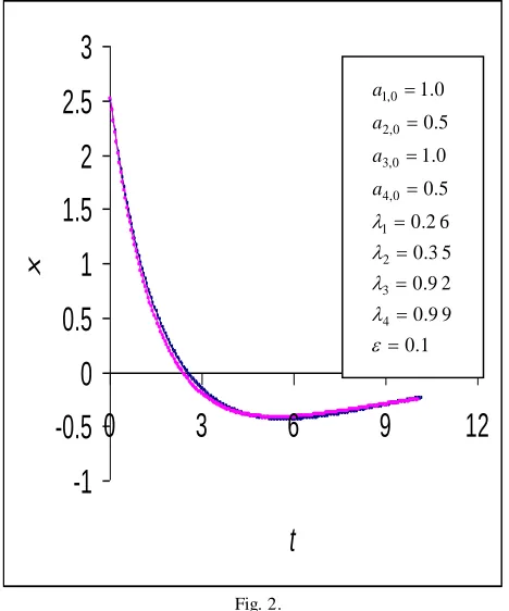
The approximate solution obtained by the presented technique of this article has been compared to the numerical solution to test the accuracy. First,
x
(
t
,
)
is calculated by (24) by using the imposed conditions that
1
2,
3
3
1 and
4
3 in which4 3 2
1
,
a
,
a
,
a
a
are calculated by the equation (23). The corresponding numerical solution of (11) is computed by fourth order Runge-Kutta method. The approximate analytic solutions and numerical solutions are plotted in the figure Fig.1 and Fig. 2. From the figures we observe that the analytical solution and the numerical solution are in nice coincidence.1112701-4646 IJBAS-IJENS © February 2011 IJENS
-1
-0.5
0
0.5
1
1.5
2
2.5
3
0
3
6
9
12
t
x
Fig. 1.
Comparison between analytical solution and numerical solution for chosen values of arbitrary constants, eigenvalues and small parameter (analytical solution in solid line ― and numerical solution in circles line
).-1
-0.5
0
0.5
1
1.5
2
2.5
3
0
3
6
9
12
t
x
Fig. 2.
Comparison between analytical solution and numerical solution for chosen values of arbitrary constants, eigenvalues and small parameter (analytical solution in solid line ― and numerical solution in circles line
).V. CONCLUSION
An asymptotic method, based on the theory of Krylov -Bogoliubov-Mitropolskii, is developed for solving the fourth order near critically damped nonlinear systems under some conditions with small nonlinearities, when the four eigenvalues of the corresponding linear equation are real and negative numbers. The relations limit
1
2,1
3
3
and
4
3 among the eigenvalues are imposed to solve the systems. The results obtained by this method agree nicely with those obtained by the numerical method.REFERENCES
[1] Akbar, M. A., Paul A. C. and Sattar M. A., An Asymptotic Method of Krylov-Bogoliubov for Fourth Order Over-damped Nonlinear Systems, Ganit, J. Bangladesh Math. Soc., Vol. 22, pp. 83-96, 2002. [2] Akbar, M. A., Uddin, M. S., Islam, M. R. and Soma, A. A., Krylov
-Bogoliubov-Mitropolskii (KBM) Method for Fourth Order More Critically Damped Nonlinear Systems, J. Mech. of Continua and Math. Sciences Vol. 2(1), pp. 91-107, 2007.
[3] Alam, M. S. and Sattar M. A., An Asymptotic Method for T hird Order Critically Damped Nonlinear Equations, J. Mathematical and Physical Sciences, Vol. 30, pp. 291-298, 1996.
[4] Alam, M. S., Asymptotic Methods for Second Order Over-damped and Critically Damped Nonlinear Systems, Soochow Journal of Math. Vol. 27, pp. 187-200, 2001.
[5] Alam, M. S., Asymptotic Method for Non -oscillatory Nonlinear Systems, Far East J. Appl. Math., Vol. 7, pp. 119-128, 2002. [6] Alam, M. S., Asymptotic Method for Certain T hird-order
Non-oscillatory Nonlinear Systems, J. Bangladesh Academy of Sciences, Vol. 27, pp. 141-148, 2003.
[7] Bellman, R., Perturbation T echniques in Mathematics, Physics and Engineering, Holt, Rinehart and Winston, New York, 1966. [8] Bogoliubov, N. N. and Mitropolskii Yu., Asymptotic Methods in the
T heory of Nonlinear Oscillations, Gordan and Breach, New York, 1961.
[9] Krylov, N. N. and Bogoliubov N. N., Introduction to Nonlinear Mechanics, Princeton University Press, New Jersey, 1947. [10] Minorsky, N., Nonlinear oscillations, Van Nostrand, Princeton, N. J.,
pp. 375, 1962.
[11] Murty, I. S. N., and Deekshatulu B. L., Method of Variation of Parameters for Over-Damped Nonlinear Systems, J. Control, Vol.
9, no. 3, pp. 259-266,1969.
[12] Murty, I. S. N., Deekshatulu B. L. and Krishna G., On an Asymptotic Method of Krylov-Bogoliubov for Over-damped Nonlinear Systems, J. Frank. Inst., Vol. 288, pp. 49-65, 1969. [13] Nayfeh, A. H., Perturbation Methods, John Wiley and Sons, New
York, 1973.
[14] Popov, I. P., A Generalization of the Bogoliubov Asymptotic Method in the Theory of Nonlinear Oscillations (in Russian), Dokl. Akad. USSR Vol. 3, pp. 308-310, 1956
[15] Rahman, M. H.,Haque, B. M. I., and Akbar, M. A., Asymptotic Solutions of Fourth Order Near Critically Damped Nonlinear Systems, Journal of Informatics and Mathematical Sciences, Vol. 1, no. 1, pp. 61-73, 2009.
Mailing Address:
Md. Asraful Alom Lecturer
Dept. of Mathematics
Khulna University of Engineering & T echnology Khulna-9203, Bangladesh
Email: [email protected]
1 . 0
25 . 1
15 . 1
48 . 0
44 . 0
75 . 0
75 . 0
75 . 0
75 . 0
4 3 2 1 0 , 4 0 , 3
0 , 2 0 , 1
a a a a
1 . 0
9 9 . 0
9 2 . 0
3 5 . 0
2 6 . 0
5 . 0
0 . 1
5 . 0
0 . 1
4 3 2 1 0 , 4
0 , 3
0 , 2
0 , 1
Md. Habibur Rahman Assistant Professor Dept. of Mathematics
Khulna University of Engineering & T echnology Khulna-9203, Bangladesh
Email: [email protected]
B. M. Ikramul Haque Assistant Professor Dept. of Mathematics
Khulna University of Engineering & T echnology Khulna-9203, Bangladesh
Email: [email protected]
Dr. Md. Ali Akbar Assistant Professor