An Analytical
Study of Computation and
Communication Tradeo
ffs
in Distributed Graph
Processing
Systems
Amirreza Abdolrashidi
1,∗, Lakshmish Ramaswamy
11DepartmentofComputerScience,TheUniversityofGeorgia,Athens,Georgia,USA
Abstract
Distributedvertex-centricgraphprocessingsystemssuchasPregel,GiraphandGPShaveacquiredsignificant popularity in recent years. Although the manner in which graph data is partitioned and placed on the computationalnodeshasconsiderableimpactontheperformanceofthevertex-centricgraphprocessingcluster, thereareveryfewcomprehensivestudiesonthistopic.Towardsenhancingourunderstandingofthisimportant factor, in this paper, we propose a novel model for analyzing the performance of such clusters. Using three graph algorithms as case studies, we also characterize the inherenttradeoff between thecomputational load distributionandthecommunicationoverheadsofaBSPcluster.Thispaperalsoreportsadetailedexperimental study investigatingthe performance of commonly-used graph partitioning mechanisms with respect to their computationalload distributioncharacteristicsandtheassociatedcommunicationoverheads.
Receivedon 18 February 2015;acceptedon 04 July 2015;publishedon17 December 2015
Keywords: Distributed Vertex-Centric Graph Processing, Performance Modeling, Parallel Processing, Graph Partitioning.
Copyright© 2015 Amirreza Abdolrashidi and Lakshmish Ramaswamy, licensed to EAI. This is an open access article
distributed under theterms of the Creative Commons Attribution license (http://creativecommons.org/licenses/
by/3.0/), which permitsunlimiteduse, distributionand reproduction in any medium so long as the original work is
properlycited.
doi:10.4108/eai.17-12-2015.150810
1. Introduction
Many emerging domains are characterized by massive graph-structured data. Graphs with millions of nodes and billions of edges are not uncommon in applications such as WWW, bioinformatics, and social networks. These emerging applications have spurred renewed research into efficient and scalable graph analytics. Since traditional centralized graph computation has inherent scalability limitations, recent research has focused on on harnessing the parallelism offered by shared nothing clusters for graph analytics. While some of the early works explored using the MapReduce (MR) paradigm, it was soon realized that MR is not well suited for this domain because of the highly iterative nature of many graph algorithms.
Recent research suggests that bulk synchronous parallel (BSP) model is better suited for parallelizing graph algorithms on shared nothing clusters. Accordingly, many BSP-based graph processing
∗Corresponding author. Email:[email protected]
frameworks have been designed and developed in the past few years. These include Pregel [1], Giraph [2], GraphLab [3] and GPS [4]. These
vertex-centric frameworks regard individual
vertices of the graph as the fundamental units of computation. The computation logic is expressed as a series of iterations, called supersteps. In a given superstep, each vertex performs certain computations, which involve processing messages that it received from the previous superstep, updating its own state and sending messages to its neighboring vertices. The synchronization occurs at the end of each superstep.
Many factors influence the performance of vertex-centric BSP frameworks including the number of machines in the cluster, their relative capabilities, the characteristics of underlying network, and the nature of the graph computation algorithm. This paper focuses on another performance factor that has hitherto received less research attention but nevertheless has a significant impact on the performance of vertex-centric graph processing clusters, namely the manner in which the
1
EA
EAI Endorsed Transactions
on
Collaborative Computing
Research
Article
EAI Endorsed Transactions on Collaborative Computing 11-122015|Volume1|Issue5|e5
graphdataispartitionedandplacedonvariousmachines
ofthe cluster.Thisfactorisuniquelyimportantbecause
graph partitioning and placement not only affect the amountof communication that needsto happen at the end ofeach superstepbut also thecomputationalloads placedonthemachinesduring thecomputation.
Random and min-cut are two commonly adopted graphpartition and placement strategies. As the name suggests, the random strategy distributes the vertices of the graph to the compute nodes in a random fashion.Min-cut, ontheotherhand,aimstoreduce the communication in the cluster bydistributing the nodes in a way that minimizes the number of inter-partition edges (edges whose end vertices are allocated to two differentpartitionsand,hence,assignedto twodifferent computenodes).However,tothebestofourknowledge, there arenocomprehensivestudiesabouttheimpactof these or other graph partitioning strategies on cluster performance.
Analyzing the impact of graph partitioning on the communication and computation loads of a vertex-centric BSP cluster is quite challenging because it is intertwined with other performance factors such as the cluster setup, communication and computation capabilities of various nodes in the cluster and the natureofthegraphcomputation.Inthispaper,wemake three important contributions towards addressing this importantchallenge:
• First, we propose a novel analytical model for vertex-centric graph cluster performance. This model incorporates an important and diverse set of performance parameters such as computational loads on processors, messaging loads between pairs of processors and available computation and communication resources within the cluster. A unique aspect of our model is that it can be used to analyze and compare different graph partitioning strategies.
• Second, we highlight the tradeoffs between computational load distribution on the processors of a BSP cluster and the communication loads within the cluster. We discuss three distinct graph algorithms and illustrate how the above tradeoff manifests differently in each algorithm.
• Third, we introduce novel metrics to accurately quantify the load balancing and communication characteristics of vertex-centric graph computa-tions. We have also conducted a detailed experi-mental study involving massive real world graphs (millions of vertices and edges) on Amazon EC2 clusters with a varying number of compute nodes. This experimental study highlights the relative benefits and costs of random and min-cut graph
partitioning strategies with respect to communi-cation overheads and computational load distribu-tions.
The remainder of the paper is organized as follows: In section??, we provide a brief discussion on vertex-centric graph processing model of computation. In section3, we describe the performance cost of this model and provide formal specifications. Section4discusses the metrics used for measuring the performance in our experiments. This section also includes the experiments’ setups and results. We briefly discuss related works in section5and conclude the paper in section6.
2. Vertex-Centric Graph Processing
Since the introduction of MapReduce [5], many systems have used this model to process large graphs [6], [7], [8], [9], [10], [11], [12] and [13]. In these systems, graph algorithms have to be modeled as a sequence of chained MapReduce jobs. However, this model is not appropriate for graph algorithms from the perspective of both data and computation model [14], [15] and [16]. Initially, the data need to be modeled as key-value pairs in order for MapReduce jobs to proceed. However, modeling graph algorithms as sequences of such functional programming constructs that operate on key-value pairs is not necessarily efficient or easy. Additionally, graph algorithms by nature are iterative where computation includes several iterations of similar operations that are performed on graph vertices. Using MapReduce to model graph algorithms will yield iterative disk intensive jobs in which the entire state of graph should be transferred from one iteration to another in order for the computation to proceed. During computation of the arbitrary graph algorithm in a large-scale environment, distribution over many machines makes memory access time as well as I/O overhead worse and, consequently, affects the performance of the framework [1].
Another computation model that has been used recently for parallel processing of large graphs is Valiant’s Bulk Synchronous Parallel (BSP) model. BSP is a “bridging model” for general purpose parallel computation [17], that is, parallelism across a wide range of applications and architectures. In the BSP paradigm, computation consists of a series of iterations named supersteps. Each superstep is divided into three phases as follows:
• Computation, where each process using local data
stored in memory of its processor performs the computation.
• Communication, where the processes send and
• Barrier Synchronization, where all the communica-tions are complete and the data sent by processors are available for the destination processors in the next superstep.
Computation based on this parallel model will finally be terminated once it goes through the desired number of supersteps, or a specific convergence criterion is met.
Pregel [1] used the above computation model to process large graphs by applying a vertex-centric approach to the implementation of graph algorithms. In this approach, vertices of the graphs are considered as the work units that are partitioned among processor nodes of a cluster. At the beginning of each superstep, in the computation phase, the processor nodes of the cluster receive messages from the previous superstep and perform the user defined logic of computation in parallel on each of the work units by running a compute method on each of the vertices. Once a processor node finishes the processing of its work units, it begins the
communication phase where it sends messages to other
vertices (possibly located at other processor nodes) along graph edges. Finally, in the synchronization phase, the processor nodes will wait for the slowest processor to finish processing and sending its messages, and then, they become synchronized. This marks the end of one superstep, and afterwards, all the processor nodes start the next superstep.
In order for the computation to terminate, graph vertices need to inform each other whether they participate in the computation. In other words, they need to be stateful. Pregel considers two states for each graph vertex along with a mechanism calledvoting
to halt (which involves graph vertices changing their
states between the two states) to achieve statefulness of vertices and subsequently mark the end of computation. Initially in the first superstep all the graph vertices are in the active state. Active graph vertices participate in the computation. After the computation on each active vertex is completed, it changes its state to inactive in order to inform other vertices that it has no further work to do. Inactive vertices will not participate in the computation in the next superstep unless they receive a message from other vertices, at which point, they will change their state back to active and will participate in the computation. The computation ends when all the graph vertices are in the inactive state and there are no messages left among vertices to process.
Vertex-centric processing of graphs with the use of BSP computational model leads to the interaction of several factors that ultimately determines the performance of the underlying cluster. In the next section, we identify these factors and provide an accurate and tractable model that describes the role of each of these elements.
♣r ♦❝❡ss♦ r❆ ♣r ♦❝❡ss♦ r❇
♣r ♦❝❡ss♦ r❈ ✶
✹
✼
✶✵ ✶✸
✶✻
✶✾ ✷ ✷
✷ ✺
✽ ✶ ✶
✶ ✹ ✶✼ ✷ ✵
✷✸
✸ ✻
✾ ✶✷
✶✺
✶✽
✷✶ ✷✹
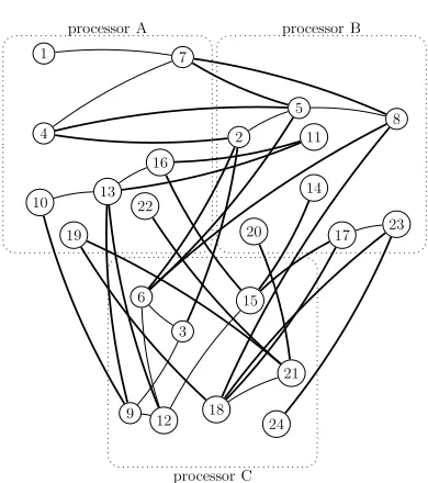
Figure 1. Random partitioning of a sample graph G(24,36)
among three processors; each processor node has 8 vertices; 24 intra-cluster edges (highlighted in bold) and 12 inter-cluster edges
3. Performance Model for Vertex-Centric
Graph Processing
In vertex-centric processing of graphs, two major factors that determine the performance of the computation are the communication cost among the processor nodes of the cluster and the computation cost of each of the processor nodes of the cluster. This is similar to other parallel computations.
As mentioned in the previous section, in the vertex-centric processing of a graph, an active vertex sends a message to another vertex if there is an edge between them. Consequently, the manner in which graph vertices are placed among processor nodes affects the communication and computation of the cluster and, hence, plays a key role in determining the performance of the cluster.
One simple approach to placement of graph vertices on processor nodes is random partitioning of graph vertices. For instance, consider Figure 1, which illustrates the distribution of a sample graph vertices on three processor nodes based on random partitioning. As depicted, each partition has the same number of vertices. In this approach the communication volume among processor nodes is high as there are many intra-cluster edges (highlighted in bold). In this manner, processor nodes need to constantly send messages among each other for the computation to proceed. Despite resulting in a higher communication cost, we will see that the advantage of such partitioning is in achieving a better load balance among processor nodes in case of some graph algorithms.
3 EAI Endorsed Transactions Collaborative Computingon
11-122015|Volume1|Issue5|e5
♣r ♦❝❡ss♦ r❆ ♣r ♦❝❡ss♦ r❇
♣r ♦❝❡ss♦ r❈ ✶
✷
✸
✹ ✺
✻ ✼
✽
✾
✶✵ ✶ ✶
✶ ✷
✶✸ ✶✹ ✶ ✺ ✶ ✻
✶ ✼ ✶✽
✶✾ ✷✵
✷ ✶
✷ ✷
✷✸
✷✹
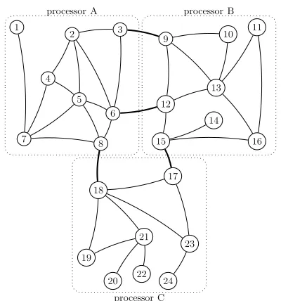
Figure 2. Min-cut partitioning of a sample graph G(24,36)
among three processors; each processor node has 8 vertices; 4 intra-cluster edges (highlighted in bold) and 32 inter-cluster edges
The other approach for placement of graph vertices on processor nodes can be applying heuristics based graph partitioning algorithms in order to compute the min-cuts of the graphs with the goal of lowering the communication cost. Figure2represents the partitioning of the same exemplary graph of Figure 1 based on results of min-cut computation. As illustrated, each highly connected partition of the graph is located on one processor node, and there are four intra-clusters edges (highlighted in bold) among processor nodes. Such an approach to placement of graph vertices on processor nodes results in lower communication cost among processor nodes. This is due to the fact that the majority of the edges (along which vertices will send messages) are accessible by each processor. Consequently, there will be fewer messages that need to be sent among processor nodes in order to access graph vertices. This approach, however, leads to load imbalance among processor nodes, as we will demonstrate later.
As exemplified in both Figs. 1 and 2, there exists a tradeoff among computation and communication costs of the cluster depending on how the graph vertices are assigned to processor nodes. Next, we will propose a formal performance cost model for vertex-centric processing of graphs on a cluster, which reflects these tradeoffs and enables analyzing the efficiency of vertex-centric graph processing algorithms.
3.1. Performance Cost Model
As described in section 2, a superstep is divided into three phases. Hence, the cost of a superstep relies on the
cost of each of its three phases: the (maximum) cost of the local computation on each processor, the (maximum) cost of the communication among processors and the cost of the barrier synchronization at the end of the superstep. Thus the cost of a superstep can be formulated as:
Cost of a Superstep= max
1≤i≤n(Comp CostPi)+
max
1≤i≤n(Comm CostPi) +l
(1)
where Comp CostPi andComm CostPi are computation cost and communication cost of the processor node i respectively and n is the number of processor nodes. In the following sections we provide formal descriptions for the cost of each of the three phases and explain the factors that affect each of them. In this paper, we use the terms “cost” and “time” interchangeably.
Computation. The cost of computation is related to
the amount of the load on the processors. In order to model the cost of the computation phase of a single superstep, the first criterion might be measuring the number of vertices that each processor has to process during that superstep.
However, this approach is naive. The reason is due to the fact that during each superstep not all vertices of a processor node are active and only the vertices that are in the active state will participate in the computation and constitute the load on a processor node. For instance, all of the processor nodes in both figures 1 and 2 have the same number of vertices, but this does not mean that they have the same amount of load because not all of the vertices might be active during a superstep. This factor depends on the behavior of the graph algorithm in terms of message passing as we will see in the next section. Thus, in order to measure the load of a processor node,Number of Active Vertices (NAV)reflects the right metric.
However, the mere measurement of the number of active vertices is not sufficient to model the load of a processor node. Another factor in determining the load is the Number of Messages that a processor needs to process at the beginning of each superstep. There can be circumstances where two processor nodes have the same number of active vertices in a superstep, but one might have to process more messages to determine the final number of active vertices that will participate in the computation. This factor depends on the underlying graph structure and the distribution of degree of the vertices. For instance, as can be seen in both figures 1 and 2, vertices 1, 14, 20, 22 and 24 have a degree of one and hence have to process one message during a superstep whereas vertices 5, 6, 13, 18 and 21 have a higher degree and have to process more messages.
formulated as:
Comp Cost(SSk) = max
1≤i≤n(AV)×α+ max1≤i≤n(di×γ)×β (2) where the first factor is the maximum number ofActive
Vertices(AV) overn processor nodes multiplied by cost
of main operation α of computation (e.g. addition of multiplication) and the second factor is the maximum number of messages that a graph vertex with input degree d might receive with probability γ times β, the cost of processing a message by processor. It should be noted that in the first superstep the second factor would be zero because there would be no messages to receive and process from the previous superstep.
Communication. The second factor that determines
the time of a single superstep is the length of the communication phase.
Since the processors in the cluster communicate in parallel, this time is the maximum time it takes the communication network to deliver messages among processors. This cost is related to the maximum number of bytes that have to be sent or received during a superstep and also is dependent on available network bandwidth. We model this cost formally as:
Comm Cost(SSk) = max
1≤i≤n(SentBytesPi,RcvdBytesPi)/g
(3) where the nominator of the fraction is the maximum number of bytes to be sent or received by processor i amongn processors andgis network bandwidth.
Synchronization. The final determining factor of time
of a superstep is the time it takes for all processor nodes to become synchronized and ready for the execution of the subsequent superstep. This is a constant cost that is dependent on the cost of sending a single message across the diameter of the network in order to synchronize processor nodes. We will not measure this cost in our experiments and consider it asl.
Considering the above equations, we measure the time of a single superstep when processing a vertex-centric graph computation as follows:
Cost(Superstep)= max
1≤i≤n(AV)×α+ max1≤i≤n(di×γ)×β + max
1≤i≤n(SentBytesi,RcvdBytesi)/g+l
(4)
3.2. Tradeoffs between Computation and
Communication
Considering equation 4, it is evident that in vertex-centric parallel graph processing the interaction of computation cost on each processor node and communication cost among them are the two major
factors that can affect the performance of such clusters. These two factors are also related to both placement of graph vertices and the nature of graph algorithm computation in terms of their message passing behavior. In the processing of algorithms in which communica-tion among vertices is intensive and vertices constantly send messages to each other, communication determines the performance of parallel clusters. In such compu-tations, lowering communication cost is an important criterion. Applying heuristic-based algorithms such as min-cut to place the vertices among processor nodes will lead to better results for this criterion and consequently improve the performance.
On the other hand, there are graph algorithms the computations of which are not communication intensive. Therefore, the determining factor of the performance is the computation costs of the processors. To improve this factor, the load should be evenly distributed among processor nodes. Random assignment of graph vertices to processor nodes can be a candidate to meet this goal. In next section, we consider different graph algorithms and show the differences in terms of their message passing behaviors when a vertex-centric approach is used to implement them.
3.3. Graph Algorithms
We begin our discussion by providing the pseudo codes for three graph algorithms, namely the PageRank [18], Dijkstra’s algorithm for the Single Source Shortest Path problem [19] (SSSP, here after) and the Weakly Connected Components (WCC, here after) which is similar to the distributed version of the HCC (Highly Connected Components) mentioned in [7], in Alg. 1, 2 and 3, respectively. These graph algorithms behave differently in terms of message passing among graph vertices. In vertex-centric parallel processing of a graph, a vertex changes its state to active upon receiving a message from the previous superstep. Thus, the manner in which a graph vertex sends messages to other vertices can be different for different graph algorithms.
As seen in Alg.1 (line 13) during the computation of PageRank, a vertex changes its state to inactive when the maximum number of supersteps is reached. Otherwise, it will continue to update its value and participate in computation. In other words, in each superstep, the vertices of the graph are active, and they continue to send messages to their neighbors. The computation of PageRank will terminate when the maximum number of provided supersteps has been executed and finished.
On the other hand, as shown in Alg.2, an SSSP vertex will vote to halt whenever its value does not update to a newer one (line 10). Otherwise, it will update its value with the new shortest distance from the source vertex. By becoming active, it will also send messages to its neighbors and inform them about it updated
5 EAI Endorsed Transactions Collaborative Computingon
11-122015|Volume1|Issue5|e5
Algorithm 1Vertex-Centric Implementation of PageRank
1: functionComputePR(msgs,superstep)
2: ifvrtx has no ngbrthen
3: V ote to Halt
4: end if
5: ifsuperstep≥1then
6: sum←0
7: formsg in msgsdo
8: sum←sum+msg.val
9: end for
10: numV rts = len(ngbrs) 11: prV al←P R(sum, nmV rts) 12: sendM sg(ngbrs, numV rts)
13: ifsuperstep = maxSuperStepthen
14: V ote to Halt
15: end if
16: end if
17: end function
value. The computation of the SSSP algorithm might not necessarily terminate when exactly the predefined number of supersteps is reached. It might end earlier due to the above mentioned message passing behavior.
Alg. 3 shows the pseudo code of the Weakly Connected Components (WCC). The approach used for computation of the WCC is as follows: During multiple iterations of the WCC algorithm, vertices send their labels to each other and then store the maximum value that they have received until their convergence criterion is met. In vertex-centric implementation of the WCC, in first superstep, the vertices begin the computation by assigning their IDs to their component IDs (the identifier that shows which component a vertex belongs to). Then, they send this value to the vertices that they are connected to. In the next supersteps, the vertices update their component IDs to the value of the component ID that they have received the most up to that point. If this value (component ID) gets updated, they inform their neighbors by sending the updated value to them. Otherwise, they become inactive and do not participate in the computation. This kind of message passing behavior is similar to that of SSSP where
Algorithm 2Vertex-Centric Implementation of SSSP
1: functionComputeSSSP(msgs,superstep)
2: ifIsSource(vID)then
3: minDis←0
4: else
5: minDis← ∞
6: end if
7: formsg in msgsdo
8: mindDis = min(mindDis , msg.val)
9: end for
10: ifminDis≤vrtxV althen
11: vrtxV al←minDis
12: sendM sg(ngbrs, vrtxV al) 13: else
14: V ote to Halt
15: end if
16: end function
Algorithm 3 Vertex-Centric Implementation of WCC
1: functionComputeWCC(msgs,superstep)
2: ifIsFisrtSuperstep(superstep)then
3: wccID←vID
4: sendM sg(ngbrs, wccID) 5: else
6: formsg in msgsdo
7: recwccID←getwccID(msg)
8: updatewccCounter(recwccID, wccCounter)
9: end for
10: maxSeenwccID=maxSeen(wccCounter)
11: ifwccID6=maxSeenwccIDthen
12: wccID←maxSeenwccID
13: sendM sg(ngbrs, wccID)
14: else
15: V ote to Halt
16: end if
17: end if
18: end function
the computation might end before it goes through the maximum number of provided supersteps. However, in SSSP, the computation begins from a single source vertex and moves throughout the topology of the graph until its termination, whereas in computation of the WCC, all of the vertices become active at the beginning of the first superstep and, depending on the manner in which their component IDs get updated, might participate in the next phases of computation or not.
3.4. Illustration of Tradeoffs
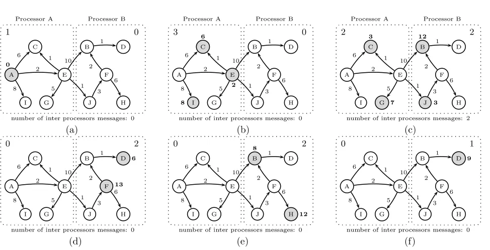
Pr ♦❝ ❡ss♦r❆ Pr ♦❝ ❡ss♦r❇
❆ ✵
❈
■
❊
●
❇
❋
❏
❉
❍ ✻
✽ ✷
✶
✺ ✶
✶ ✸ ✷
✻ ✶
✁ ✂
♥✉♠❜❡r♦❢✐♥t❡r♣r ♦ ❝❡ss♦rs♠❡ss❛❣❡ s✿ ✭✄ ✮
Pr ♦ ❝❡ss♦r❆ Pr ♦ ❝❡ss♦r❇
❆ ❈ ☎
■ ✆
❊ ✝ ●
❇
❋
❏
❉
❍ ✻
✽ ✷
✶
✺ ✶
✶ ✸ ✷
✻ ✶
✞ ✂
♥✉♠❜❡r♦❢✐♥t❡r♣r ♦ ❝ ❡ ss♦r s♠❡ ss❛❣❡ s✿ ✭ ✟✮
Pr ♦ ❝❡ss♦r❆ Pr ♦ ❝❡ss♦r❇
❆ ❈ ✠
■
❊
● ✼ ❇ ✡ ✝
❋
❏ ✠ ❉
❍ ✻
✽ ✷
✶
✺ ✶
✶ ✸ ✷
✻ ✶
☛ ☛
♥✉♠❜❡ r♦❢✐♥t❡ r♣r ♦❝ ❡ss♦r s♠❡ss❛❣❡s✿✷ ✭ ☞✮
❆ ❈
■
❊
●
❇
❋ ✡✠
❏
❉ ☎
❍ ✻
✽ ✷
✶
✺ ✶
✶ ✸ ✷
✻ ✶
✂ ☛
♥✉♠❜❡r♦❢✐♥t❡r♣r ♦ ❝❡ss♦rs♠❡ss❛❣❡ s✿ ✭ ❞ ✮
❆ ❈
■
❊
●
❇ ✆
❋
❏
❉
❍ ✡ ✝ ✻
✽ ✷
✶
✺ ✶
✶ ✸ ✷
✻ ✶
✂ ☛
♥✉♠❜❡r♦❢✐♥t❡r♣r ♦ ❝ ❡ ss♦r s♠❡ ss❛❣❡ s✿ ✭ ✌ ✮
❆ ❈
■
❊
●
❇
❋
❏
❉ ✾
❍ ✻
✽ ✷
✶
✺ ✶
✶ ✸ ✷
✻ ✶
✂ ✁
♥✉♠❜❡ r♦❢✐♥t❡ r♣r ♦❝ ❡ss♦r s♠❡ss❛❣❡s✿ ✭ ✍✮
Figure 3. Execution of SSSP on Graph G(10,11) when graph vertices are partitioned based on result of min-cut.
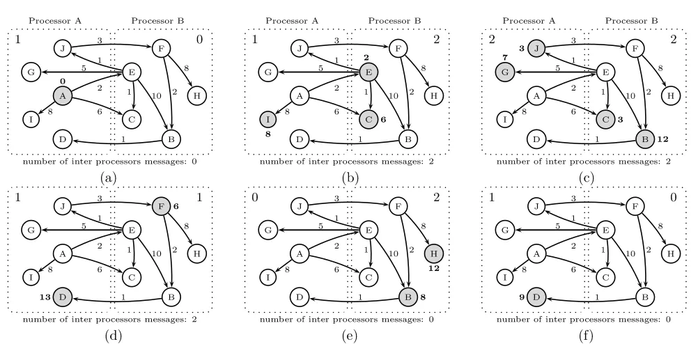
‘J’ become active by receiving messages from vertex ‘E’ that has sent two messages from the first processor to the second processor. The computation continues until the last superstep where vertex ‘D’ updates its value (Figure 3.f), and then since there is no active vertex, it will terminate. As can be seen in 3, one processor is always idle since no active vertex resides on it and does not participate in the computation.
Figure 4 depicts the same computation on the same graph where the vertices are partitioned among two processor nodes at random. In the first superstep (Figure 4.a), vertex ‘A’ is active and starts the computation. The vertex sends messages to its neighbors. In second superstep, the vertices residing on it become active and hence the processor node performs the computation. The computation proceeds by nodes exchanging their states from active to inactive and updating their values. However, the number of supersteps in which only one processor node is participating in computation is half compared to that of the min-cut approach (figures4.a,4.e and 4.f). Such adjustment comes with a greater number of messages that are sent among processor nodes.
Table 1 summarizes the above example of existing tradeoffs between computation and communication costs of vertex-centric parallel processing of graphs. In the second column, we show the ratio of number of supersteps in which only one processor node contains the active vertice(s) to the total number of supersteps for the execution of the SSSP. This ratio is a measure of load imbalance. The last column displays the total number of messages that are sent between two processor nodes during execution of the SSSP. The communication
Table 1. Summary of tradeoffs between Communication
and Computation cost for the SSSP example
Ratio of♯of imbalanced Total♯of
Partitioning supersteps to total messages sent among
♯of supersteps processor nodes
Min-cut 5/6 2
Random 3/6 6
cost is related to the communication cost. As depicted, minimizing the amount of communication can create a significant load imbalance, which is a determinant of the overall system’s performance.
4. Experimental Evaluation
In this section, we define new performance metrics for better quantifying the computational load distribution among the nodes of a vertex-centric BSP cluster and the communication load within the cluster. We also discuss the experiments we have performed and their results.
4.1. Performance Metrics
The existence of the cost model that is both tractable and accurate makes it possible to analyze efficiency of graph algorithms when the vertex-centric programming model is utilized. As shown in eq. 4, the following strategies should be considered in order to achieve high efficiency for a superstep time:
• balance the computation in each superstep among processors for two reasons. First, we must consider the maximum number of active vertices and the
7
EAI Endorsed Transactions on Collaborative Computing 11-122015|Volume1|Issue5|e5
Pr ♦❝ ❡ss♦r❆ Pr ♦❝ ❡ss♦r❇ ❆ ✵ ● ❏ ■ ❉ ❈ ❊ ❋ ❇ ❍ ✽ ✻ ✷ ✺ ✶ ✶ ✶ ✸ ✽ ✷ ✶ ✁ ✂
♥✉♠❜❡r♦❢✐♥t❡r♣r ♦ ❝❡ss♦rs♠❡ss❛❣❡ s✿ ✭✄ ✮
Pr ♦ ❝❡ss♦r❆ Pr ♦ ❝❡ss♦r❇
❆ ● ❏ ■ ☎ ❉ ❈ ✆ ❊ ✝ ❋ ❇ ❍ ✽ ✻ ✷ ✺ ✶ ✶ ✶ ✸ ✽ ✷ ✶ ✁ ✞
♥✉♠❜❡r♦❢✐♥t❡r♣r ♦ ❝ ❡ ss♦r s♠❡ ss❛❣❡ s✿ ✷ ✭ ✟✮
Pr ♦ ❝❡ss♦r❆ Pr ♦ ❝❡ss♦r❇
❆ ● ✼ ❏ ✠ ■ ❉ ❈ ✠ ❊ ❋ ❇ ✡✝ ❍ ✽ ✻ ✷ ✺ ✶ ✶ ✶ ✸ ✽ ✷ ✶ ✞ ✞
♥✉♠❜❡ r♦❢✐♥t❡ r♣r ♦❝ ❡ss♦r s♠❡ss❛❣❡s✿✷ ✭ ☛✮ ❆ ● ❏ ■ ❉ ✡ ✠ ❈ ❊ ❋ ✆ ❇ ❍ ✽ ✻ ✷ ✺ ✶ ✶ ✶ ✸ ✽ ✷ ✶ ✁ ✁
♥✉♠❜❡r♦❢✐♥t❡r♣r ♦ ❝❡ss♦rs♠❡ss❛❣❡ s✿ ✷ ✭ ❞ ✮ ❆ ● ❏ ■ ❉ ❈ ❊ ❋ ❇ ☎ ❍ ✡✝ ✽ ✻ ✷ ✺ ✶ ✶ ✶ ✸ ✽ ✷ ✶ ✂ ✞
♥✉♠❜❡r♦❢✐♥t❡r♣r ♦ ❝ ❡ ss♦r s♠❡ ss❛❣❡ s✿ ✭ ☞ ✮ ❆ ● ❏ ■ ❉ ✾ ❈ ❊ ❋ ❇ ❍ ✽ ✻ ✷ ✺ ✶ ✶ ✶ ✸ ✽ ✷ ✶ ✁ ✂
♥✉♠❜❡ r♦❢✐♥t❡ r♣r ♦❝ ❡ss♦r s♠❡ss❛❣❡s✿ ✭ ✌✮
Figure 4. Execution of SSSP on Graph G(10,11) when nodes are randomly partitioned.
number of messages among processors. Second, in the barrier synchronization phase, processors must wait for the slowest processor to complete its computation.
• balance the communication among processor nodes since the maximum of received bytes and sent bytes of data is taken among processor nodes.
In order to measure the load balance of a superstep in terms of both of the factors (number of active vertices and number of messages to receive) that affect the computation phase of a superstep, we define the following metrics. For the first factor, we define the average of standard deviations of number of active vertices over all supersteps to be the first metric to measure the performance of load balance as follows:
Load Balanceav(N,K,A)=
K P k=1 ( s N P i=1
(AV(Pik)−µ)2
N )
K (5)
where Load Balanceav(N,K,A) is the load balance of
N processor nodes during K supersteps when running graph algorithm A (in terms of number of active
vertices), AV(Pik) is the number of active vertices for
processori at superstepkand µ is the average number of active vertices on processor nodes in superstepk.
Similarly for the second factor of load balance, we define the following metric:
Load Balancerm(N,K,A)=
K P k=1 ( s N P i=1
(RM(Pik)−µ)2
N )
K (6)
where Load Balancerm(N,K,A) is the load balance of
N processor nodes during K supersteps when running graph algorithm A (in terms of number of received
messages), rm(Pik) is the number of received messages
for processoriat superstepkandµis the average number of received messages by all processor nodes in superstep k. In order to measure the cost of the communication phase among N processor nodes during K supersteps when running graph algorithmA, we define the following metric which is the sum of the averages of sent and received bytes.
Comm Cost(N,K,A)=
K X k=1 ( N P i=1
(SentBytes(Pik)
N )+ K X k=1 ( N P i=1
(ReceivedBytes(Pik)
N )
(7)
4.2. Experimental Setup
In order to measure the performance of vertex-centric graph algorithms in terms of the above metrics, we have performed extensive experiments on different graph datasets. The graph dataset information is shown in table 2. The first three datasets (web-Stanford, Amazon0601 and web-Google) are from [20]; the rest are obtained by using Webgraph software [21].
and communication cost on clusters with different sizes. Each node in our cluster is an Amazon’s “m3.medium” instance type with single core high frequency Intel Xeon E5-2670 v2 cpu, 3.75 GB of memory running Ubuntu Server 14.04. The performance of our communication network among processor nodes is set at a moderate level. We also have used GPS to implement vertex-centric the implementation of PageRank, SSSP and WCC graph algorithms as provided in Algorithms1, 2and 3.
As the baseline for our experiments, first we examine the random partitioning of graph vertices on processor nodes. In this scenario, the graph vertices are randomly placed on the processor nodes of clusters and no structural properties of the graph are examined for the placement of the graph vertices on cluster nodes. In our experiments we refer to this approach as RND. We also used the Metis [22] graph partitioning software to partition the graphs and then distribute the graph vertices among processor nodes based on the results of Metis graph partitioning software. Metis uses multilevel k-way partitioning algorithms to compute the min-cut of a graph. Metis’ heuristic-based algorithms try to find the best partitions where the number of inter-partitions (cuts) are minimum while each partition holds the same number of vertices. The idea here is that by performing min-cut the communication cost of the cluster will be lowered. We partitioned the graph so that each partition has the same number of vertices while the number of cross cluster edges are minimal. Then we assigned each graph partition to a processor node. As we will see in section 5, however, lowering communication cost using Metis will result in lower load balance for SSSP and WCC graph algorithms. We referred to this graph partitioning scheme asMTS in our experiments.
4.3. Results
Load Balancing. In terms of the first performance
metric for load balancing (Load Balanceav) as shown
Table 2. Graph Datasets Information
Name of Graph Vertices Edges Description
web-Stanford 281,903 2,312,497 Web graph of
Stanford.edu
Amazon0601 403,394 3,387,388
Amazon product co-purchasing
network from
June 1 2003
web-Google 875,713 5,105,039 Web graph from
in-2004 1,382,908 16,917,053 the .in domain of
WWW graph
itwiki-2013 1,016,867 25,619,926
the italian part of Wikipedia as late as Feb 2013
ljournal-2008 5,363,260 79,023,142
LiveJournal virtual
community social site
in Figure 5, when the graphs are partitioned randomly the load is evenly distributed among processor nodes. However, when the graph vertices are distributed among processors based on graph partitioning scheme (Metis) the load of processors is very unbalanced as it is shown with high values for average of standard deviation for active vertices (see Eq. 5 for definition of this metric). Figure 5 depicts the results for this metric for the PageRank, SSSP and WCC algorithms for six different graph datasets. As shown in this Figure, the load is evenly distributed if the graph vertices are randomly distributed among processor nodes compared to the case when vertices are assigned to processors based on the results of Metis. For instance, during computation of PageRank algorithm for web-Stanford dataset (shown in Figure 5.a) when the graph is partitioned between two compute nodes in a random fashion, the average of standard deviation for number of active vertices is 1. However, when the graph is partitioned between two nodes based on the result of Metis, the same performance metric will be 4,021. It is also noticeable that as the number of processor nodes in the cluster increases from 2 to 16 the load imbalance decreases to almost half (for instance from 7,349 for two nodes to 479 for sixteen nodes in the case of in-2004 dataset and from 254,433 for two nodes to 1,713 for sixteen nodes in the case of itwiki-2013 dataset) when PageRank algorithm is computed. Consequently, a possible solution for having a more balanced load among processor nodes when running a graph algorithm such as PageRank is to add more nodes to the cluster.
In the case of the SSSP algorithm, the load balance worsens as the number of processor nodes increases from 2 to 16 (for all graph datasets except ljournal-2008). This is because during execution of the SSSP algorithm the computation starts at some region of the graph, and it propagates to other regions of the graph until it terminates. Hence, the load balancing of this graph algorithm in terms of active vertices is sensitive to the starting vertex (source vertex) of the computation. For ljournal-2008, however, this is not true since the starting vertex for this graph is in a very dense part of the graph where, by adding more nodes to the cluster, the load on processor nodes becomes more balanced, and hence, the average of standard deviation across supersteps becomes lower. Similarly to the circumstances for PageRank, random partitioning always outperforms the assignment of graph vertices to processor nodes based on Metis in terms of average standard deviation of active vertices across supersteps.
Considering the computation of the WCC, we can see that adding more compute nodes has a similar effect to the SSSP on the first metric of load balancing for different graph datasets. For instance, for itwiki-2013 graph dataset (Figure 5.e) the value for performance metric5 is 11,136 when the graph is partitioned among
9 EAI Endorsed Transactions
on Collaborative Computing 11-122015|Volume1|Issue5|e5
0 1000 2000 3000 4000 5000
PageRank SSSP WCC
Load Balance
av
web-Stanford
RND-2Nodes
1 26 24
MTS-2Nodes
4021
1007
871
RND-4Nodes
0 20 22
MTS-4Nodes
2407
1812
1441
RND-8Nodes
0 18 19
MTS-8Nodes
1085
2611
2225
RND-16Nodes
0 20 16
MTS-16Nodes 479 3514 3637 0 1000 2000 3000 4000 5000 6000 7000
PageRank SSSP WCC
Load Balance
av
Amazon0601
RND-2Nodes
0 30 28
MTS-2Nodes
5884
1236
715
RND-4Nodes
1 28 27
MTS-4Nodes
2689
2165
1280
RND-8Nodes
0 30 26
MTS-8Nodes
1219
3605
2789
RND-16Nodes
0 22 23
MTS-16Nodes 683 4525 4647 0 1000 2000 3000 4000 5000 6000 7000
PageRank SSSP WCC
Load Balance
av
web-Google
RND-2Nodes
0 28 27
MTS-2Nodes
6262
542
374
RND-4Nodes
0 24 21
MTS-4Nodes
4894
1036
709
RND-8Nodes
1 22 17
MTS-8Nodes
2435
1447 1495
RND-16Nodes
0 18 14
MTS-16Nodes
747
1783
2601
a) web-Stanford b) Amazon0601 c) web-Google
0 1000 2000 3000 4000 5000 6000 7000 8000
PageRank SSSP WCC
Load Balance
av
in-2004
RND-2Nodes
0 32 28
MTS-2Nodes
7349
751 634
RND-4Nodes
0 31 21
MTS-4Nodes
4994
1207 1047
RND-8Nodes
1 23 24
MTS-8Nodes
3653
1941 1837
RND-16Nodes
1 19 20
MTS-16Nodes 1379 2195 2745 0 50000 100000 150000 200000 250000
PageRank SSSP WCC
Load Balance
av
itwiki-2013
RND-2Nodes
1 20 50
MTS-2Nodes
254433
3358 11136
RND-4Nodes
0 25 66
MTS-4Nodes
220283
23046
13942
RND-8Nodes
0 20 60
MTS-8Nodes
14834
26704
16226
RND-16Nodes
0 15 51
MTS-16Nodes 1713 31067 19053 0 10000 20000 30000 40000 50000 60000 70000 80000
PageRank SSSP WCC
Load Balance
av
ljournal-2008
RND-2Nodes
0 56 231
MTS-2Nodes
78232
21735
11193
RND-4Nodes
0 47 197
MTS-4Nodes
39088
12586 15572
RND-8Nodes
1 32 132
MTS-8Nodes
17754
6412
35784
RND-16Nodes
0 23 137
MTS-16Nodes
9276
3603
54210
d) in-2014 e) itwiki-2013 f) ljournal-2008
Figure 5. Load Balanceav performance metric for web-Stanford, Amazon0601, web-Google, in-2004, itwiki-2013 and
ljournal-2008 datasets
two compute nodes based on the results of Metis. However, when the number of compute nodes increases to sixteen (again, partitioning based on the results of Metis), this metric has the value of 19,053.
The results for the second performance metric of the load balance (Load Balancerm) is depicted in Figure 6.
Similarly to the first metric for the load balance, randomly assigning graph vertices to the processor nodes leads to a lower average of standard deviations across supersteps for the number of received messages by processors as compared to instances in which a graph partitioning scheme such as Metis is used. This is because of the correlation between the number of active vertices and received messages and the fact that the graph vertex changes its state from inactive to active upon receiving messages. This also demonstrates that, when graph partitioning mechanisms such as Metis are used, the load among processors is distributed unevenly in terms of the active vertices that processors have to handle in order to perform the computation.
In conclusion, as it is shown both in Figure 5 and 6, the random assignment of graph vertices to processor of
clusters leads to better load distribution among processor nodes of a cluster compared to when a graph partitioning scheme such as Metis is used. However, as we will see in the next section, using Metis has advantages in terms of communication cost of the cluster when the nature of the graph algorithm requires high communication among processors. We also notice that one way to have better load balancing in a cluster is to add more nodes to the cluster.
Communication. For the performance metric related
0 200 400 600 800 1000 1200 1400
PageRank SSSP WCC
Load Balance rm web-Stanford RND-2Nodes 190 0 16 MTS-2Nodes 1484 11 241 RND-4Nodes 167 1 36 MTS-4Nodes 1019 17 337 RND-8Nodes 125 0 59 MTS-8Nodes 729 28 614 RND-16Nodes 101 1 72 MTS-16Nodes 314 38 723 0 500 1000 1500 2000 2500 3000
PageRank SSSP WCC
Load Balance rm Amazon0601 RND-2Nodes 229 1 31 MTS-2Nodes 3053 20 496 RND-4Nodes 195 3 56 MTS-4Nodes 2167 29 572 RND-8Nodes 141 2 68 MTS-8Nodes 1906 37 837 RND-16Nodes 117 3 81 MTS-16Nodes 827 47 998 0 1000 2000 3000 4000 5000 6000
PageRank SSSP WCC
Load Balance rm web-Google RND-2Nodes 238 1 52 MTS-2Nodes 6109 23 818 RND-4Nodes 202 3 67 MTS-4Nodes 5839 35 1199 RND-8Nodes 165 3 76 MTS-8Nodes 4362 41 1671 RND-16Nodes
131 5 87
MTS-16Nodes
2834
49
1893
a) web-Stanford b) Amazon0601 c) web-Google
0 1000 2000 3000 4000 5000 6000 7000 8000
PageRank SSSP WCC
Load Balance rm in-2004 RND-2Nodes 249 1 65 MTS-2Nodes 7655 31 880 RND-4Nodes 216 1 72 MTS-4Nodes 7287 44 1491 RND-8Nodes 179 1 81 MTS-8Nodes 6060 48 1853 RND-16Nodes
147 0 93
MTS-16Nodes 5798 53 2017 0 10000 20000 30000 40000 50000
PageRank SSSP WCC
Load Balance
rm
itwiki-2013
RND-2Nodes
641 3 97
MTS-2Nodes
47841
50 1462
RND-4Nodes
528 3 103
MTS-4Nodes
41423
192
2149
RND-8Nodes
337 2 159
MTS-8Nodes
2381
165
4467
RND-16Nodes
323 1 192
MTS-16Nodes 1947 253 9669 0 10000 20000 30000 40000 50000 60000 70000 80000
PageRank SSSP WCC
Load Balance
rm
ljournal-2008
RND-2Nodes
404 1 159
MTS-2Nodes
84480
265
30180
RND-4Nodes
250 1 99
MTS-4Nodes
46018
200
20637
RND-8Nodes
157 1 62
MTS-8Nodes
28214
119
11733
RND-16Nodes
83 1 56
MTS-16Nodes
14278
91
3313
d) in-2014 e) itwiki-2013 f) ljournal-2008
Figure 6. Load Balancerm performance metric for web-Stanford, Amazon0601, web-Google, in-2004, itwiki-2013 and
ljournal-2008 datasets
processor node does not need to send a message across the cluster to another node as it holds the neighboring vertices.
In the case of the SSSP and WCC algorithms, the benefits of using a graph partitioning solution such as Metis is not very significant since the graph algorithm is not very intensive in terms of communication volume. As mentioned before, the computation of the SSSP algorithm starts at a source vertex and the communication among graph vertices initiates at a local region of the graph that contains the source vertex. The communication among vertices then propagates throughout the graph structure until all the graph vertices update their value (shortest distance from source). This marks the end of the SSSP computation. Compared to the PageRank algorithm, the SSSP computation involves less communication.
In conclusion, as it is shown in Figure 7, when the communication volume of the graph algorithm in terms of bytes the network has to deliver to processor nodes is very high, the application of the graph partitioning solution is beneficial to the communication cost of the
network. However, this solution leads to load imbalance as we saw previously in Figure5 and6.
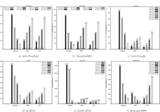
Time. Figure8 shows the total time of completion for
three graph algorithms for clusters with different sizes when random partitioning and Metis based partitioning is used. The bar graphs in this figure reveal several findings. First, for PageRank computation of all datasets, as the number of nodes in the cluster increases, the total time of completion decreases and execution is completed faster. This is because of better load balancing both in terms of number of active vertices and received messages (as shown previously in Figure5and6).
Second, when the graph algorithm has a high volume of communication (e.g. PageRank), using Metis in order to decrease the communication cost leads to a significant benefit in terms of faster execution time. This reveals the fact that, in the case of the PageRank computation for these three datasets, communication among processor nodes is the dominant factor in determining the ultimate cost of execution.
Third, for the computation of the SSSP and the WCC algorithms, as shown in the middle and right parts of the
11
EAI Endorsed Transactions on Collaborative Computing 11-122015|Volume1|Issue5|e5
0 5 10 15 20 25 30
PageRank SSSP WCC
Communictation (MB) web-Stanford RND-2Nodes 13.86 .51 5.01 MTS-2Nodes 4.34 0.01 1.84 RND-4Nodes 20.81 .63 8.93 MTS-4Nodes 7.72 0.02 2.52 RND-8Nodes 24.26 .74 10.21 MTS-8Nodes 9.41 0.03 3.97 RND-16Nodes 26.01 .89 11.03 MTS-16Nodes 10.75 0.04 4.21 0 5 10 15 20 25 30 35 40
PageRank SSSP WCC
Communictation (MB) Amazon0601 RND-2Nodes 21.12 .63 13.91 MTS-2Nodes 6.01 0.01 3.67 RND-4Nodes 31.44 .75 20.70 MTS-4Nodes 8.32 0.02 4.82 RND-8Nodes 36.30 .80 23.91 MTS-8Nodes 10.03 0.03 5.42 RND-16Nodes 38.50 .93 25.35 MTS-16Nodes 12.86 0.04 6.96 0 10 20 30 40 50 60 70 80
PageRank SSSP WCC
Communictation (MB) web-Google RND-2Nodes 36.63 1.28 14.92 MTS-2Nodes 7.32 0.13 5.13 RND-4Nodes 51.93 1.72 22.38 MTS-4Nodes 10.53 0.16 6.21 RND-8Nodes 59.59 2.01 26.11 MTS-8Nodes 12.61 0.18 7.06 RND-16Nodes 66.36 2.06 27.47 MTS-16Nodes 14.38 0.19 8.38
a) web-Stanford b) Amazon0601 c) web-Google
0 50 100 150 200 250
PageRank SSSP WCC
Communictation (MB) in-2004 RND-2Nodes 102.80 0.81 42.31 MTS-2Nodes 32.32 0.01 5.24 RND-4Nodes 153.91 1.21 57.78 MTS-4Nodes 39.68 0.02 11.59 RND-8Nodes 176.96 1.33 72.07 MTS-8Nodes 47.84 0.03 15.87 RND-16Nodes 200.47 1.47 86.01 MTS-16Nodes 58.31 0.04 21.73 0 50 100 150 200 250 300 350
PageRank SSSP WCC
Communictation (MB) itwiki-2013 RND-2Nodes 155.61 1.91 52.33 MTS-2Nodes 42.44 .51 13.98 RND-4Nodes 232.62 2.82 78.22 MTS-4Nodes 64.43 .62 22.87 RND-8Nodes 270.51 3.21 90.90 MTS-8Nodes 71.73 .64 26.05 RND-16Nodes 288.98 4.07 97.16 MTS-16Nodes 84.65 .73 29.23 0 200 400 600 800 1000
PageRank SSSP WCC
Communictation (MB) ljournal-2008 RND-2Nodes 481.03 4.51 230.20 MTS-2Nodes 83.41 .41 22.85 RND-4Nodes 716.64 6.60 343.04 MTS-4Nodes 91.41 .85 43.85 RND-8Nodes 831.55 7.80 397.73 MTS-8Nodes 116.73 1.13 55.07 RND-16Nodes 885.93 8.2 423.98 MTS-16Nodes 121.18 1.39 60.99
d) in-2014 e) itwiki-2013 f) ljournal-2008
Figure 7. Communication Costperformance metric for web-Stanford, Amazon0601, web-Google, in-2004, itwiki-2013 and
ljournal-2008 datasets
graphs, it is evident that when Metis based partitioning of graph vertices to the processor nodes is applied the total time of completion is longer compared to random partitioning. In fact, utilizing graph partitioning has a negative effect on the performance of the system. The explanation for this phenomenon is depicted in the results of load balancing as well as communication cost for this graph partitioning scenario. As shown in Figure 7, the achieved benefit in terms of lowering the communication volume is insignificant when Metis is used for the SSSP graph algorithm. On the other hand, the load imbalance in terms of both number of active vertices and received messages is high for the SSSP and the WCC when Metis is used (Figure 5 and 6). These two factors (low benefit of graph partitioning and high load imbalance) lead to higher completion time for all datasets.
Finally, it is noticeable in Figure 8 that the time of completion for the SSSP also increases as more nodes are added to the cluster. This reemphasizes that the number of active vertices and received messages by the processors
(load) is the dominant factor in determining the total run time of the SSSP.
5. Related Work
The extensive body of research in the field of distributed processing of large graphs covers a variety of topics including different computational models, graph storage and query processing, static and dynamic graph partitioning, minings and analysis of social networks data, etc. Here, we will review the contributions to the field that are closely related to our work. First, we will review the contributions and trends in algorithms for graph partitioning. Then, we will review different systems and frameworks, as well as computational models for processing large graphs.
5.1. Graph Partitioning Applications and Methods
0 10 20 30 40 50 60
PageRank SSSP WCC
Time (Seconds) web-Stanford RND-2Nodes 48.4 22.8 29.6 MTS-2Nodes 38.2 24.8 33.2 RND-4Nodes 37.4 23.3 31.4 MTS-4Nodes 29.9 26.4 36.0 RND-8Nodes 27.7 24.6 33.1 MTS-8Nodes 21.1 28.0 38.8 RND-16Nodes 19.9 25.9 35.6 MTS-16Nodes 17.8 31.7 41.1 0 10 20 30 40 50 60 70
PageRank SSSP WCC
Time (Seconds) Amazon0601 RND-2Nodes 57.1 26.3 34.7 MTS-2Nodes 43.1 30.8 39.1 RND-4Nodes 40.1 24.7 32.6 MTS-4Nodes 30.1 28.7 36.3 RND-8Nodes 27.7 31.6 34.9 MTS-8Nodes 29.6 35.4 38.7 RND-16Nodes 25.1 34.9 36.2 MTS-16Nodes 20.4 39.1 41.4 0 20 40 60 80 100 120 140
PageRank SSSP WCC
Time (Seconds)
web-Google
RND-2Nodes
83.2 81.7 84.8
MTS-2Nodes 66.6 85.8 88.2 RND-4Nodes 62.7 87.4 89.3 MTS-4Nodes 47.9 91.3 93.1 RND-8Nodes 46.0 89.3 84.8 MTS-8Nodes 36.7 93.9 97.3 RND-16Nodes 34.9 92.6 96.7 MTS-16Nodes 28.8 96.9 102.2
a) web-Stanford b) Amazon0601 c) web-Google
0 20 40 60 80 100 120 140
PageRank SSSP WCC
Time (Seconds) in-2004 RND-2Nodes 94.1 99.3 96.7 MTS-2Nodes 76.1 108.2 106.1 RND-4Nodes 72.2 97.6 98.1 MTS-4Nodes 55.2 105.9 108.9 RND-8Nodes 56.2 103.5 101.0 MTS-8Nodes 47.2 111.4 112.1 RND-16Nodes 45.8 107.6 102.9 MTS-16Nodes 33.5 116.1 115.3 0 50 100 150 200
PageRank SSSP WCC
Time (Seconds) itwiki-2013 RND-2Nodes 164.1 71.2 114.6 MTS-2Nodes 144.1 78.2 124.8 RND-4Nodes 150.4 70.3 116.4 MTS-4Nodes 100.2 78.4 126.2 RND-8Nodes 129.4 74.9 119.8 MTS-8Nodes 65.3 81.1 129.5 RND-16Nodes 101.2 79.3 124.8 MTS-16Nodes 30.7 86.4 133.1 0 100 200 300 400 500 600 700
PageRank SSSP WCC
Time (Seconds) ljournal-2008 RND-2Nodes 589.2 133.2 220.3 MTS-2Nodes 519.2 143.2 235.3 RND-4Nodes 303.2 119.2 226.6 MTS-4Nodes 278.1 129.3 243.1 RND-8Nodes 159.2 103.5 232.4 MTS-8Nodes 143.2 117.5 253.1 RND-16Nodes 114.7 97.8 256.7 MTS-16Nodes 101.9 106.6 271.7
d) in-2014 e) itwiki-2013 f) ljournal-2008
Figure 8. Timeperformance metric for web-Stanford, Amazon0601, web-Google, in-2004, itwiki-2013 and ljournal-2008
datasets
subproblem that has extensive applications in many different areas including parallel scientific computing and mesh partitioning ([23], [24], [25], [26]), power grids design ([27], [28], [29]), biological networks analysis ([30], [31]), social networks analysis ([32], [33]), road networks design ([34], [35], [36], [37], [38], [39]), image processing([40], [41]) and VLSI design ([42], [43]).
Graph partitioning is an NP-Complete problem, however, there are many algorithms that find near optimal solutions. These methods and techniques can be classified into two broad groups,Static methods and
Dynamic ones.
Static Graph Partitioning Methods. Static Graph
partitioning involves partitioning of the vertices of a graph in p roughly equal partitions such that the number of edge cuts (edges connecting vertices in different partitions) is minimized. In this class of graph partitioning methods, the global information about the graph is known and the structure of the graph is stable and does not change. One well known class of methods for static graph partitioning is spectral partitioning methods that are used extensively, and
are known to produce good partitions. These methods were first pioneered by [44], [45] and [46] and involve the computation of the eigenvector (Fielder vector) corresponding to the second smallest eigenvalue of the Laplacian matrixLof the graph. However, these methods are very expensive in terms of computation and further improvements were introduced in works of [47], [48], [49] and [50]. In [49], a multilevel spectral bisection method is introduced for fast approximation of the Fielder vector that leads to an order of magnitude faster solution time with no loss in the quality of edge cuts.
Another type of static graph partitioning techniques utilizes the geometric information of the graph vertices in space to find good solutions. Although these algorithms ([51], [52], [53], [54], [55]) tend to be fast, they often find partitions that are worse compared to those yielded by spectral methods. The more promising in this class of algorithms are [52] and [53] that use recursive coordinate bisections to map the graph vertices onto coordinate axis with the longest expansion of domains. Applications of geometric graph partitioning algorithms are limited to the graphs in which the coordinates of their nodes
13 EAI Endorsed Transactions on Collaborative Computing 11-122015|Volume1|Issue5|e5
are available. These applications include finite elements models and graphs from traditional scientific computing where the information about the geometry of the nodes are known. However, in the field of VLSI design and integer programming where such information is not available, geometric algorithms are not applicable.
Multilevel static graph partitioning schemes are another class of techniques that have shown to be the most successful solutions for partitioning large graphs. The idea in these methods is to coarsen the graph by collapsing the vertices and edges, partition the smaller graph and finally uncoarsen the graph to construct a partition for the original graph ([56], [57], [58], [59], [60], [61] and [62]). The goal of coarsening (or contraction) phase is to gradually decrease the size of the original graph by creating a hierarchy of consecutive graphs that are decreasing in size in a manner that partitions (cuts) of the coarsened graphs indicate the partitions (cuts) of the fine graph in higher levels of hierarchy. Multiple heuristics have been proposed for this step including Random Maximal Matching [56], Light Edge Matching and Heavy Edge Matching [63], [64]. The contraction phase terminates when graph is small enough to utilize a fast, efficient and near optimal technique such as Kernighan-Lin algorithm [65] to compute the initial partitions. During the uncoarsening phase, two steps will take place. First, the solution of the coarsened graph is projected on to the fine graph at the higher level. Second, using different metaheuristics such as node-swapping local search such as [66] or [67] further improvements are provided on quality of partitions. These two steps are performed during the uncoarsening phase until the finest level of hierarchy (original graph) has been processed.
Intuitively speaking, the multilevel graph partitioning algorithms perform so well for several reasons. First, by grouping the vertices of the graph together during the coarsening phase, the granularity at which the graph partitioning heuristics will be applied is increased. In other words, partitioning the coarsened graph results in the partitioning of lots of graph vertices without escalating the execution time. Second, the movement of a single node during the coarsening phase results in a lot of change in the final solution. Thus, it would be easier to find improvements at this level compared to finest level. Third, because solutions at coarser level yield good results as starting points for next level in hierarchy during uncoarsening phase, the improvments at finer level are expected to run faster. These methods can also be easily parallelized because the global solution is achieved by local processings [68], [69].
Similar to the above idea of multilevel graph partitioning, the authors in [70] have proposed a framework based on label propagation that enables partitioning of a billion node graph. In this system, the graph iteratively is coarsened by the result of the
label propagation. Then, once the graph size is sufficient, a graph partitioner will partition the graph and, the result is projected back to the graph. This framework is applicable for static graphs and is not suitable when the topology of the graph changes.
The authors in [71] considered the problem of static graph partitioning for large scale-free (power law) graphs. They have shown the benefits of the two-dimensional (edge partitioning) graph partitioning methods over the one-dimensional (vertex partitioning) layouts by performing an empirical comparison of several distributions of each of the above categories for the problem of sparse matrix-vector multiplication on large scale-free graphs. They also have proposed a new two-dimensional graph partitioning scheme that exploits the information in the graph structure and the topology which outperforms other edge partitioning methods for the problem of sparse matrix-vector multiplication.
Dynamic Graph Partitioning Methods. In dynamic
graph partitioning, the structure of the graph changes with time and only local information about parts of the vertices and edges of the graph might be available. These algorithms assign edges and vertices based on the local information they have. Their goal is to find a close-to-optimal balanced partitioning with minimal memory usage and computational overhead while maintaining good edge cuts compared to that of static graph partitioning methods.
5.2. Big Graphs Processing Systems and
Computational Models
Bulk Synchronous Parallelism (BSP) was first introduced at [17] as a computational model for general purpose parallelism. Its fundamental properties are being able to write simple parallel programs that are independent of target architecture and also having predictable performance on a given architecture. Pregel [1] was the first system to extend this computational model to graph processing and is a proprietary product of Google. In this system, efficient, scalable and fault-tolerant implementation of the BSP model is utilized on clusters of thousands of nodes. Google has introduced a simple API that facilitates writing vertex-centric graph algorithms that can be used on their cluster.
Apache Giraph [2] is an open source counterpart of the Pregel that is in use at Facebook to analyze their social graph data formed by its users and their interactions. Compared to basic Pregel, Giraph has several additional features such as master computation and out of core computation.
GraphLab [3] is another computation abstraction that was developed by Carnegie Mellon University and is tailored for machine learning tasks. Their computational model is different than BSP as they use asynchronous message passing among processors in order to achieve a high degree of parallel performance in their machine learning tasks.
PowerGraph [74] is a distributed adaptation of GraphLab. In this work, the authors have targeted processing of graphs with power-law degree distribution. High efficiency of processing such graphs in this system is achieved by introducing a new vertex-partitioning model as well a novel programming model, namely Gather-Apply-Scatter (GAS). This programing model is conceptually very similar to that of Pregel, however, it utilizes the internal structure of the graphs to partition the vertices among processor nodes.
GraphChi [75] is a system that has been introduced for efficiently processing graph algorithms. The computation model of GraphChi is vertex-centric. However, it is based on a single machine, and it accomplishes computation of different graph analytics using sequential disk access with a parallel sliding window method. This method implements the asynchronous model of computation and resembles the single machine based version of GraphLab. This is an advantage over synchronous manner of computation of BSP (and Pregel-like) system as the convergence of graph algorithms can accelerate.
Spark [76] is another framework that extends MapReduce model of computation in order to support iterative machine learning and graph algorithms. This extension is done through introduction of a read-only collection of resilient distributed datasets (RDDs). These datasets can be placed across a set of machines running
MapReduce and have the ability to recover a partition if lost.
Pegasus [7] utilizes a MapReduce model of compu-tation. It models iterative graph algorithms as general-ized matrix-vector multiplications. It then uses different methods such as block multiplication, clustered edges and diagonal block iteration (that are based on the features of a matrix) to achieve faster performance compared to a single MapReduce job. However, its performance is lower than systems that are based on message passing.
Trinity [77] is a framework for general purpose computation of different online graph query answering and offline graph analytics over the cloud. It achieves high performance by providing a distributed low latency key value graph storage where data is stored in a binary format. Trinity provides a more restrictive but similar model of computation to Pregel in which a vertex can only send messages to fixed number of vertices (usually neighbors). This restrictive model is used in offline graph algorithms. The rationalization behind this restrictive design decision is two-fold. First, the authors have observed that the computation of many offline algorithms can be accomplished by limiting the access of vertices to their neighbors. Second, it provides the opportunity to predict the communication pattern among graph vertices during each iteration which enables optimization of network communication.
Mizan [78] follows the Pregel model of computation and is implemented in C++. It provides dynamic load balancing and vertex migration based on monitoring the results of vertex computation. This provides the opprotunity to optimize the computation by reducing the communication cost among the compute nodes. Mizan uses the Metis graph partitioning software before distributing the graph vertices and edges among the compute nodes, which can lead to lower performance compared to other systems such as Giraph.
Kineograph [79] considers the problem of graph processing from a different perspective. It is a distributed computing engine to support execution of different graph mining algorithms on time-evolving graphs. It creates a constantly changing graph from a stream of data with relationships among the entities in datasets and then uses the proposed new epoch commit protocol to build different consistent and static snapshots of the graph to be used by graph-mining algorithms. The authors have performed different experiments to analyze Twitter data feeds including user ranking, approximating the shortest path between users and detection of disputed topics at rates higher than reported peaks of Twitter and reported different levels of guarantees for response time for different rates of tweets as well as cluster sizes. In [80], the authors have made an experimental comparison among vertex-centric graph processing systems. They proposed a framework for comparisons
15 EAI Endorsed Transactions Collaborative Computingon
11-122015|Volume1|Issue5|e5
among four open-source Pregel-like systems and measured different performance metrics including memory and network bandwidth usage and running time. They also have discussed different aspects of each system in terms of ease of use and development of graph data processing.
Ligra [81] (LIghtwieght Interface for GRaph Algo-rithms) differs from above-mentioned systems in several ways. First, compared to the other systems, Ligra is designed for shared memory multicore machines where a graph with tens or even hundreds of billions of vertices and edges can fit into the shared memory. The benefit of utilizing a single multicore server of that caliber for processing large graphs is the significant reduction of communication costs. Second, Ligra is well suited for graph traversal problems such as shortest paths, graph radii estimation, graph connectivity and betweenness centrality. The authors have focused on Breadth-First Search (BFS) like algorithms where at each iteration of algorithm a subset of vertices are considered. For this types of graph algorithms, they have proposed a new abstraction called Vertex Subset. They also have proposed two other constructs for mapping vertices
(Vertex Map) and mapping edges (Edge Map) and have
developed different graph algorithms based on these constructs. However, they have not mentioned what kind of graph partitioning has been used in their system.
In [82] a new parallel abstraction named Blogel has been proposed to address the bottlenecks of Pregel-like systems when processing large graphs with three main characteristics. The examined graphs in this work have three main attributes including skewed degree distribution, large diameter and (relatively) high density. To overcome the poor performance of vertex-centric system when processing such graphs, Blogel works with collectivized units of graphs. More specifically, the level of abstraction in Blogel is blocks of graphs where a block is a connected subgraph of the original graph. The idea behind Blogel is that by considering blocks of graphs as units of processing, the problems of skewed degree distribution, heavy communication due to high density and large diameter will naturally be addressed. However, a key issue in Blogel is how an arbitrary graph can be partitioned into blocks efficiently. To answer this question, a new fully distributed graph partitioning algorithm based on Voroni diagrams is proposed. The experiments reveal that the results of applying the proposed partitioning mechanism for graph abstractions at the level of blocks are promising.
Authors in [15] have compared three different types of parallel graph processing abstractions and systems in terms of their performance and reported their findings. Specifically, they have compared MapReduce, map-side join (an extension of original MapReduce) and BSP implementations of the single source shortest path and collective classification of graph vertices by use of
Relational Influence Propagation. The latter algorithm is type of graph node classification based on label propagation and is similar to [70] and [83]. Their results show that the BSP implementation of these two graph algorithms outperform both MapReduce and its improved extension (map-side join) by an order of magnitude in terms of performance. Compared to BSP, MapReduce in an alternative that provides the capability of processing immense graph whose size is larger than memory of a BSP cluster.
Performance evaluation of different graph processing systems have led to the benchmark proposed in [84] where several performance metrics are introduced for various platforms. More specifically, a broad process of representing different performance metrics, across seven graph datasets for various graph algorithms have been defined. The performance metrics include resource utilization and scalability and are measured for six different systems including [85], [86], [87], [3], [88] and [2]. Apart from MapReduce and Bulk Synchronous Parallel models of computation, Stratosphere [89] is another platform for large scale processing of graph datasets. Stratosphere’s design is based on the amalgamation of MapReduce programming model and the Dyrad [90] distributed data processing engine. In other words, Stratosphere consists of two major components. The parallel data processing engine of Stratosphere is Nephele [91] where jobs and the dataflow among them are modeled using Directed Acyclic Graphs (DAG), a similar job modeling to the distributed platform [90]. Pact [88] is the programming model of Stratosphere which is an extension of MapReduce to support more flexible dataflow. In addition to map and reduce functions, Pact provides second-order functions such as Match and Cross as well as several code annotations by user that informs the Pact compiler about the expected behavior of such added functions.
There have also been several works on the vertex-centric approaches to different applications such as graph pattern matching and simulation where given a query graph Q and a distributed data graph G, a graph pattern matching algorithm has to find matches of graph Q in G. In [92], different versions of this problem are considered. More specifically, the authors in [92] developed different heuristics such as graph simulation, dual simulation, strong simulation and strict simulation based on a vertex-centric BSP based model of computation where they have achieved high performance compared to centralized approaches.