Outage Performance of a Two-branch Cooperative
Energy-constrained Relaying Network with Selection
Combining at Destination
Sang Quang Nguyen
1,∗, Hyung Yun Kong
21Institute of Fundamental and Applied Sciences, Duy Tan University, Ho Chi Minh City 700000, Vietnam
2Department of Electrical Engineering, University of Ulsan, Korea
Abstract
In this paper, we investigate two-branch cooperative DF relaying networks with selection combining at the destination. Two intermediate relay-clusters (a conventional relay cluster and an energy-constrained relay cluster) are utilized to aid the communication between the source and the destination. We study two cases: direct link (DR) and no direct link (NDR) between the source and the destination. In each case, we consider two relay selection schemes: best sourceâĂŞrelay channel gain (BSR) and random relay selection (RAN). Thus, we have 4 protocols: DR-BSR, DR-RAN, NDR-BSR, and NDR-RAN. For the performance evaluation, we derive a closed-form expression for the outage probability of each of the four protocols. Our analysis is substantiated via a Monte Carlo simulation. As expected, the results show that the DR case outperforms the NDR case, and the BSR scheme outperforms the RAN scheme. The outage performances of the protocols are evaluated based on the system parameters, including the transmit power, the number of relays in each cluster, the energy harvesting efficiency, the position of the two clusters, and the target rate. The outage performance of the system is improved when the transmit power increases, the energy harvesting efficiency increases, the distance between the two clusters and the source and destination decreases, or the target rate decreases. We found good matches between the theoretical and Monte Carlo simulation results, verifying our mathematical analysis.
Keywords: Cooperativecommunication,Energyharvesting,Decode-and-forward,Powersplitting,Selectioncombining
1. Introduction
In wireless communication, cooperative diversity is a promising technique used to enhance data rates and reliability, in which a source transmits data to a destina-tion with the help of relays leading to acquire benefits from both relayed communications and space diversity
[1]. The concept of cooperative communication was first
investigated in [2]. Cooperation expands the coverage
area of a cellular system, compared to non-cooperation,
as demonstrated in [3]. Two well-known relaying
pro-tocols are used in cooperative communication: decode and forward (DF) and amplify and forward (AF). In the AF protocol, the cooperating node or relay node ampli-fies and forwards the source signal to the destination, whereas in the DF protocol, the signal is decoded at the relay node, and it is then re-encoded and forwarded to the destination. The implementation of the AF protocol
∗
Corresponding author. Email:[email protected]
is simpler than the DF protocol, but along with the signal, the noise is also amplified and forwarded to the
destination. In [4] and [5], the authors derived
closed-form expressions for symbol error probability (SEP),
bit error rate (BER), achievable spectral efficiency, and
outage probability of a dual-hop DF relaying network over a Rayleigh fading channel and a Nakgami-m fad-ing channel, respectively. The analysis of a dual-hop two-way semi-blind AF relay network (partial chan-nel state information (CSI)) was investigated in terms of average sum-rate, outage probability, and average
symbol error rate over Rayleigh fading channels [6],
Nakagami-m fading channels [7], and generalized-k
fading channels [8]. The authors in [9] studied the
hybrid AF-DF protocol, in which some relays amplify the received signal and others decode and forward the signal, for mutltihop relaying networks. The authors
in [10] investigated the performance of dual-hop DF
relaying networks under the joint impact of hardware impairment and co-channel interference.
Research Article
EAI Endorsed Transactions
on Industrial Networks and Intelligent Systems
Received on 04 May 2018, accepted on 16 May 2018, published on 27 June 2018
Copyright © 2018Sang Quang Nguyen and Hyung Yun Kong, licensed to EAI. This is an open access article distributed under the terms of the Creative Commons Attribution licence (http://creativecommons.org/licenses/by/3.0/), which permits unlimited use, distribution and reproduction in any medium so long as the original work is properly cited.
Diversity combining is a practical technique to effi -ciently combine multiple received signals at the des-tination receiver in both source-desdes-tination and relay-destination communication links. Selection combining (SC) and maximal ratio combining (MRC) are two advantageous and popular linear combining schemes
[11]-[12]. The MRC scheme achieves full diversity
by compiling the signal-to-noise ratios (SNRs) of all received signals, but its implementation requires many multipliers and adders, leading to higher implementa-tion complexity and cost for mobile devices than the SC schemes that choose only the strongest diversity path (the received signal with the highest SNR). The performance of the DF relaying system with selection
combining has been widely studied [13]-[17].
Recently, wireless information and power transfer technology has become an attractive solution for prolonging the lifetime of energy-constrained wireless devices by enabling each of them to simultaneously harvest energy and process information from the
ambient radio frequency (RF) signals [18]-[21], [27],
[28]. Two practical energy harvesting architectures for
simultaneous wireless information and power transfer are power-splitting (PS) and time-switching (TS). The PS receiver splits the received signal into two parts according to a power splitting ratio, one part for harvesting the energy and the other one for information processing. The TS receiver harvests energy from the received signal during an initial interval in a time block and then switches to processing the information during the remaining interval of this time block. Several works have investigated the application of energy harvesting techniques in energy-constrained
relay nodes in cooperative wireless networks. In [22],
the authors evaluated the performance of a dual-hop AF relaying system under both PS and TS architectures in terms of outage probability, throughput, and ergodic
capacity. In [23], the authors analyzed the throughput
performance of three proposed wireless power transfer policies in two-way energy-constrained AF relaying networks. The performance of an energy-harvesting relaying network with the assistance of multiple relay
nodes was studied in [24]. In [25], the authors derived
the exact outage probability for a DF energy-harvesting
relaying network with N-th best relay selection and
considering both PS and TS architectures.
To the best of our knowledge, no study has considered a cooperative system model aided by two groups of relays: conventional relay and energy-constrained relay, and applying diversity combining at the destination. This motivates us to analyze the closed-form outage probability for this model. In this model, we consider the communication between a source and a destination assisted via two groups of DF relays (two relay clusters), in which the first group consists of multiple conventional relay nodes, and the second group
includes multiple energy-constrained relay nodes. We also consider the direct source-destination link. Two relay selection schemes, i.e., best source-relay channel gain selection (BSR) and random selection (RAN), are presented in this paper. The best relay in each cluster is selected following the BSR or RAN strategy to help relay the source information to the destination: the best relay in the conventional relay cluster decodes the source signal, re-encodes, and then forwards to the destination; the best relay in the energy-constrained relay cluster harvests the energy, decodes the information from the received signal, and then re-encodes and forwards it to the destination. We present both cases: direct link (DR) and no direct link (NDR) between the source and destination. Therefore, we have four protocols: DR-RAN, DR-BSR, NDR-RAN, and NDR-BSR. At the destination, the selection-combining (SC) technique is utilized to combine three received signals in the DR case, or to combine two received signals in the NDR case. To conduct performance evaluation and comparison, we derive closed-from expressions for the outage probabilities of the four protocols, and we verify these analyses via Monte Carlo simulations.
This paper is arranged as follows. A description of the system model is presented in Section 2. Section 3 presents the operation principles. In Section 4, the closed form expressions for the RAN and BSR schemes in the DR case are derived. The closed-form expressions for the NDR case are presented in Section 5. Numerical and simulation results are discussed in Section 6. Section 7 provides the conclusions for this work.
Notation: The notationCN(a, b) denotes a circularly symmetric complex Gaussian random variable (RV)
with meanaand varianceb.E {.}denotes mathematical
expectation. The functions fX(.) and FX(.) present
the probability density function (PDF) and cumulative
distribution function (CDF) of RV X. The function
Γ(x, y) is an incomplete Gamma function [26, Eq.
(8.350.2)].Cba= a!(bb−!a)!.
2. System model
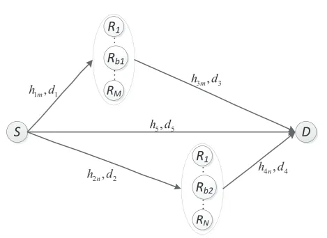
As shown in Figure 1, we consider a cooperative two-branch relaying network, which includes a source
node S, an energy-constraint relay cluster comprising
M nodes Rm (m= 1,2, ..., M), a conventional relay
cluster comprising N nodes Rn (n= 1,2, ..., N), and a
destination nodeD. Here, there is a direct link available
fromStoD. Thus, the communication fromStoDcan
occur via three paths: direct transmission, viaRm, and
via Rn. In the network, all nodes are equipped with a
single antenna operating in half-duplex mode [25]
In Fig. 1, (h1m, d1m), (h2n, d2n), (h3m, d3m), (h4n, d4n),
and (h5, d5) denote the Rayleigh fading channel
coefficients and distances of the links S−Rm, S−
.
.
.
S
..
R
1
R
b1
R
M
.
.
.
D
.
.
.
..
.
R
1
R
b2
R
N
.
.
.
1m,
1h
d
2n
,
2h
d
3m
,
3h
d
4n
,
4h
d
5
,
5h d
Figure 1. System model
dω=
˜ dω Dω,ω
∈ {1m,2n,3m,4n,5}, where ˜dω is the actual
distance and Dω is the reference distance. Thus, the
corresponding channel gainsgω =|hω|2are exponential
random variables (RVs) with parameter λω= (dω)β,
whereβ denotes the path-loss exponent (from 2 to 6).
We obtain the corresponding cumulative distribution function (CDF) and probability density function (PDF)
as Fgω(x) = 1−e
−λωx
and fgω(x) =λωe
−λωx
. We note that the distances between two nodes in a cluster are insignificant compared to the distance between a node inside and a node outside a cluster. Thus, we
denote d1m=d1, d2n=d2, d3m=d3, and d4n =d4 and
thenλ1m=λ1,λ2n=λ2,λ3m=λ3, andλ4n =λ4, where
m= 1,2, ..., M andn= 1,2, ..., N. The best relays in an
energy-constraint relay cluster and conventional relay
cluster, which are denoted asRb1 andRb2, are selected
by the destinationD, because D can obtain all fading
channel coefficients in the setup phase [25].
3. Operation principles
In the first time slot, the sourceS broadcasts its signal
x(t), where En|x(t)|2= 1o, with transmit power P to
all relays in the two clusters and destination D. The
received radio frequency (RF) signals at all relays and the destination are expressed as follows:
y1m(t) = √
P h1mx(t) +na1m(t) (1)
y2n(t) = √
P h2nx(t) +na2n(t) (2)
y5(t) = √
P h5x(t) +na5(t) (3)
where y1m(t) and na1m(t),y2n(t) and na2n(t), andy5(t)
and na5(t) are the received RF signal and additive
white Gaussian noise (AWGN) at them-th relay in the
energy-constraint relay cluster, at then-th relay in the
conventional relay cluster, and at the destination D,
respectively;na1m, na2n, na5 ∼ CN(0, N0).
At the energy-constrained relay cluster, the best
to split the received RF signal y1b(t) = √
P h1bx(t) +
na1b(t) into two components, i.e., one for harvesting
the energy (y1b,eh(t)) and one for decoding the
information (y1b,di(t)). These two components are
expressed respectively as [25]
y1b,eh(t) = √
ρ×y1b(t) =pρP h1bx(t) +√ρna
1b(t) (4)
y1b,di(t) = p
1−ρ×y1b(t) =
q
(1−ρ)P ×h1bx(t) +p1−ρ×na
1b(t) (5)
where h1b is the Rayleigh fading channel coefficient
of the link S−Rb1, andρ is the power-splitting ratio,
ρ∈(0,1).
The signal y1b,di(t) is converted to a sampled
baseband signaly1b,di(k) [25] as
y1b,di(k) = q
(1−ρ)P ×h1bx(k) +p1−ρ×na
1b(k) +nc1b(k) (6)
wherenc1b∼(0, N0) denotes the noise from the
convert-ing process.
In the conventional relay cluster, the best relay is
selected from theN nodes, denoted asRb2, to receive
the RF signal from the source y2b(t) =
√
P h2bx(t) +
na2b(t). Similar to (6), the sampled baseband signals at
Rb2andD, e.g.,y2b(k) andy5(k), are obtained by down
converting the received RF as
y2b(k) = √
P h2bx(k) +na2b(k) +nc2b(k) (7)
y5(k) = √
P h5x(k) +na5(k) +nc5(k) (8)
whereh2bis the Rayleigh fading channel coefficient of
the linkS−Rb2;nc
2b, nc5∼ CN(0, N0).
The received SNRs at Rb1, Rb2, and D in the first
time slot can be obtained from three sampled baseband signals in (6), (7), and (8), respectively, as follows:
ψ1=
(1−ρ)P|h1b|2
(2−ρ)N0 =ω1g1b (9)
ψ2= P|h2b|
2
2N0
=ω2g2b (10)
ψ5=
P|h5|2
2N0
=ω2g5 (11)
whereω1
∆
=(2(1−−ρρ))NP0,ω2 ∆
= 2NP
0.
The harvested energy atR1bcan be obtained from the
energy harvesting component (4) as
E1b=ηρP|h1b|2T (12)
whereηis the energy conversion efficiency,η∈(0,1);T
is the time duration for the first time slot.
In the second time slot (duration time T), R1b
forwards the source data to the destination D with
transmit powerP1bobtained from the harvested energy
in Eq. 12 as P1b=E1b/T =ηρP|h1b|2=ηρP g1b. Here,
R2b uses its own power, i.e., P, to forward the data.
The received sampled baseband signals at D that are
converted from the received RF signals transmitted by
R1bandR2bare respectively expressed as
y3b(k) = p
P1bh3bx(k) +n3ab(k) +nc3b(k) (13)
y4b(k) = √
P h4bx(k) +na4b(k) +nc4b(k) (14)
whereh3bandh4b, respectively, are the Rayleigh fading
channel coefficients of the linksRb1−D and Rb2−D;
na3b, nc3b, na4b, nc4b∼CN(0, N0).
The received SNRs of the two linksRb1−DandRb2−
Dcan be obtained respectively as
ψ3= P1b|h3b|
2
2N0
=ω3g1bg3b (15)
ψ4=
P|h4b|2
2N0 =ω2g4b (16)
whereω3
∆
= ηρP2N
0.
In this paper, we consider two relay selection methods. One is random relay selection (RAN),
in which the two best relays Rb1 and Rb2 are
randomly selected from the M nodes in the
energy-constrained relay cluster and from the N nodes in
the conventional relay cluster, respectively. In this
scheme, the PDFs of the 5 RVs g1b, g2b, g3b, g4b
and g5 are respectively expressed asfg1b(x) =λ1e
−λ1x,
fg2b(x) =λ2e −λ2x
, fg3b(x) =λ3e
−λ3x
, fg4b(x) =λ4e
−λ4x
,
andfg5(x) =λ5e
−λ5x
. And their CDFs areFg1b(x) = 1−
e−λ1x, Fg
2b(x) = 1−e
−λ2x
, Fg3b(x) = 1−e
−λ3x
, Fg4b(x) =
1−e−λ4x, andFg
5(x) = 1−e
−λ5x
.
The other relay selection method is BSR, in which the best relay at each cluster is selected based on maximizing the channel gain between the relays in each cluster and the source, expressed as follows:
Rb1= max
m=1,2,...,M
|h1m|2= max m=1,2,...,Mg1m
Rb2= max
n=1,2,...,N
|h2n|2= max n=1,2,...,Ng2n
(17)
In the BSR scheme, the PDFs and CDFs of the
two RVs g1b and g2b are changed and expressed
as fg1b(x) =Mλ1
M−1 P
m=0
CMm−1(−1)me
−(m+1)λ1x
, Fg1b(x) =
1−e−λ1xM, f
g2b(x) =N λ2 N−1
P
n=0
CNn−1(−1)
ne−(n+1)λ2x
,
Fg2b(x) =
1−e−λ2xN.
4. Performance evaluation
relay selection schemes. Diversity selection combining
is used at the destinationD; thus, the outage probability
expression can be formulated as
Pout= Pr [ψ1< ψt, ψ2< ψt, ψ5< ψt]
| {z } Pr 1
+ Pr [ψ1≥ψt, ψ2 < ψt, max(ψ3, ψ5)< ψt]
| {z } Pr 2
+ Pr [ψ1< ψt, ψ2≥ψt, max(ψ4, ψ5)< ψt]
| {z } Pr 3
+ Pr [ψ1≥ψt, ψ2 ≥ψt, max(ψ3, ψ4, ψ5)< ψt]
| {z } Pr 4
(18)
First, the term Pr 1 in Eq. 18 can be rewritten as
Pr 1 = Prhg1b< ωψ1t, g2b<
ψt ω2, g5<
ψt ω2
i
=Fg1b
ψt
ω1
Fg2b
ψt
ω2
Fg5
ψt
ω2
(19)
By using the PDF of the RVsg1b,g2b, andg5for the two
relay selection schemes RAN and BSR, we obtain term Pr 1 for each scheme, as follows:
Pr 1RAN= 1−e
−λ1ψt
ω1
!
1−e−
λ2ψt
ω2
!
1−e−
λ5ψt
ω2
!
(20)
Pr 1BSR= 1−e
−λ1ψt
ω1
!M
1−e−
λ2ψt
ω2
!N
1−e−
λ5ψt
ω2
! (21)
Second, we calculate the term Pr 2 in Eq. 18 as
Pr 2 = Prhg1b≥ ωψt1, g2b<
ψt
ω2, max(ω3g1bg3b, ω2g5)< ψt
i
=Fg2b
ψ t ω2 Pr "
g1b≥
ψt
ω1, ω3g1bg3b< ψt, ω3g1bg3b> ω2g5
#
| {z } Pr 2.1
+ Pr "
g1b≥
ψt
ω1
, ω2g5< ψt, ω3g1bg3b< ω2g5 #
| {z } Pr 2.2
(22)
The terms Pr 2.1 and Pr 2.2 are expressed as
Pr 2.1 =
∞ Z
ψt
ω1
fg1b(x1) ψt
ω3x1
Z
0
fg3b(x3)
ω3
ω2x1x3
Z
0
fg5(x5)dx5dx3dx1
(23)
Pr 2.2 = Prhg1b≥ ωψt1, g5<
ψt ω2, g3b<
ω2g5
ω3g1b i = ∞ R ψt ω1
fg1b(x1) ψt
ω2
R
0
fg5(x5)
ω2x5
ω3x1
R
0
fg3b(x3)dx3dx5dx1
(24)
Using the PDFs of the three RVsg1b,g3bandg5for the
RAN and BSR schemes, we obtain
Pr 2.1RAN=
∞ R
ψt
ω1
λ1e−λ1x1
ψt
ω3x1
R
0
λ3e−λ3x3dx3dx1
− ∞ R
ψt
ω1
λ1e−λ1x1
ψt
ω3x1
R
0
λ3e−
λ3+λ5ωω23x1
x3dx3dx1
=λ1Ω1
λ1,λω3ψ3t,
ψt ω1
−λ1λ3 ω2
λ5ω3Ω2
λ1,λω5ψ2t,
λ3ψt ω3 ,
λ3ω2
λ5ω3,
ψt ω1
(25)
Pr 2.1BSR=Mλ1
M−1 P
m=0
CMm−1(−1) m ∞ R ψt ω1
e−(m+1)λ1x
ψt
ω3x1
R
0
λ3e−λ3x3dx3dx1
− ∞ R
ψt
ω1
e−(m+1)λ1x ψt
ω3x1
R
0 λ3e
−λ3+λ5ω3
ω2 x1
x3dx
3dx1
=Mλ1
M−1 P
m=0
CMm−1(−1)m
Ω1
(m+ 1)λ1,λ3ψt
ω3 ,
ψt ω1
−λ3 ω2
λ5ω3Ω2
(m+ 1)λ1,λω5ψ2t,
λ3ψt ω3 ,
λ3ω2
λ5ω3,
ψt ω1 (26)
Pr 2.2RAN=
∞ R
ψt
ω1
λ1e−λ1x1
ψt
ω2
R
0
λ5 e−λ5x5−e−
λ5+λω33ωx12
x5
! dx3dx1
= 1−e−
λ5ψt
ω2
! e−
λ1ψt
ω1 −λ1Ω3λ1,λ5ψt
ω2 ,
λ3ψt ω3 ,
λ3ω2
λ5ω3,
ψt ω1
(27)
Pr 2.2BSR=Mλ1
M−1 P
m=0
CMm−1(−1)m
∞ R
ψt
ω1
e−(m+1)λ1x
ψt
ω2
R
0
λ5 e
−λ5x5− e−
λ5+λω33ωx12
x5
!
dx3dx1
=M
M−1 P m=0C
m M−1(−1)
m
1−e−
λ5ψt
ω2
! e−
(m+1)λ1ψt
ω1
m+1
−λ1Ω3(m+ 1)λ1,λ5ψt ω2 ,
λ3ψt ω3 ,
λ3ω2
λ5ω3,
ψt ω1 (28)
whereΩ1(ϕ1, ϕ2, ϕ3) =−
∞ P p=1
(−ϕ2) p!
p
ϕ1p−1Γ(1−p, ϕ1ϕ3)
(seeAppendix A),
Ω2(ϕ1, ϕ2, ϕ3, ϕ4, ϕ5) = (1−e−ϕ2)eϕ1ϕ4Γ(0, ϕ1(ϕ5+ϕ4))
−e−ϕ2
∞ P
q=1 (−ϕ3)
q! q 1 P l=1
θl,qϕ1l−1Γ(1−l, ϕ1ϕ5)
+ϑqeϕ1ϕ4Γ(0, ϕ1(ϕ5+ϕ4))
(seeAppendix B),
Ω3(ϕ1, ϕ2, ϕ3, ϕ4, ϕ5) = (1−e−ϕ2)ϕ4eϕ1ϕ4Γ(−1, ϕ1ϕ4) +
e−ϕ2
e−ϕ2 ∞ P
t=1 (−ϕ3) (t+1)!
t+1 t P l=1 θl,tϕ1l
−1
Γ(1−l, ϕ1ϕ5)
+ϑteϕ1ϕ4Γ(0, ϕ1(ϕ5+ϕ4))
(seeAppendix C).
Then, we can obtain the term Pr 2 for the RAN and BSR schemes by substituting Eqs. 25-28 into 22:
Pr 2RAN= 1−e
−λ2ψt
ω2
!
{Pr 2.1RAN+ Pr 2.2RAN} (29)
Pr 2BSR= 1−e
−λ2ψt
ω2
!N
{Pr 2.1BSR+ Pr 2.2BSR} (30)
Third, we calculate the term Pr 3 in Eq. 18 as
Pr 3 = Pr [ψ2≥ψt] Pr [ψ1< ψt] Pr [max(ψ4, ψ5)< ψt]
= Prhg2b≥ ωψt2
i
Prhg1b< ωψt1 i
Pr [ω2g4b< ψt, g4b> g5] | {z }
Pr 3.1
+ Pr [ω2g5< ψt, g4b< g5]
| {z } Pr 3.2
(31)
Because the PDFs of the RVs g4b and g5 in the two
schemes RAN and BSR are the same, e.g.,Fg4b,RAN(x) =
Fg4b,BSR(x) = 1−e
−λ4x and f
g5,RAN(x) =fg5,BSR(x) = 1−
e−λ5x, we obtain:
Pr 3.1RAN= Pr 3.1BSR=
ψt
ω2
R
0
fg4b(x4) x4
R
0
fg5(x5)dx5dx4
= 1−e−
λ4ψt
ω2
! − λ4
λ4+λ5 1
−e− (λ4+λ5)ψt
ω2
!
(32)
Pr 3.2RAN= Pr 3.2BSR
= 1−e−
λ5ψt
ω2
! − λ5
λ4+λ5 1
−e− (λ4+λ5)ψt
ω2
!
(33)
By substituting Eqs 32 and 33 into 31, we obtain the term Pr 3 for the two relay selection schemes:
Pr 3RAN=1−e
−λ1ψt
ω1
! e−
λ2ψt
ω2
(
1−e−
λ4ψt
ω2 −e−
λ5ψt
ω2 +e−
(λ4+λ5)ψt
ω2
)
(34)
Pr 3BSR= 1−e
−λ1ψt
ω1 !M 1
− 1−e−
λ2ψt
ω2 !N (
1−e−
λ4ψt
ω2 −e−
λ5ψt
ω2 +e−
(λ4+λ5)ψt
ω2
) (35)
Fourth, we calculate the term Pr 4 in Eq. 18 as
Pr 4 = Pr "
ω1g1b≥ψt, ω2g2b≥ψt,
max(ω3g1bg3b, ω2g4b, ω2g5)< ψt
#
=h1−Fg
2b ψt ω2 i Pr "
ω1g1b≥ψt, ω3g1bg3b< ψt,
ω3g1bg3b≥ω2g4b, g4b≥g5
#
+ Pr "
ω1g1b≥ψt, ω2g4b< ψt,
ω3g1bg3b< ω2g4b, g4b≥g5
#
+ Pr "
ω1g1b≥ψt, ω3g1bg3b< ψt,
ω3g1bg3b≥ω2g5, g4b< g5
#
+ Pr "
ω1g1b≥ψt, ω2g5 < ψt, ω3g1bg3b< ω2g5, g4b< g5
#
=h1−Fg
2b ψ t ω2 i Pr
g1b≥ ωψt1, g3b<
ψt ω3g1b, ω3g1bg3b
ω2
≥g4b, g4b≥g5
| {z } Pr 4.1
+ Pr
g1b≥ ωψt1, g4< ωψ2t, g3b< ωω23
g4b
g1b, g4b≥g5
| {z } Pr 4.2
+ Pr
g1b≥ ωψt1, g3b<
ψt ω3g1b, ω3g1bg3b
ω2
≥g5, g4b< g5
| {z } Pr 4.3
+ Pr
g1b≥ ωψt1, g5<
ψt ω2,
g3b< ωω23
g5
g1b, g4b< g5
| {z } Pr 4.4
(36)
The terms Pr 4.1 and Pr 4.2 in Eq. (36) can be expressed
in the multiple integrals form, as follows:
Pr 4.1 =
∞ R
ψt
ω1
fg1b(x1) ψt
ω3x1
R
0
fg3b(x3)
ω3x1x3
ω2
R
0
fg4b(x4)
x4
R
0
fg5(x5)dx5dx4dx3dx1
(37)
Pr 4.2 =
∞ R
ψt
ω1
fg1b(x1) ψt
ω2
R
0
fg4b(x4)
ω2 ω3 x4 x1 R 0
fg3b(x3)
x4
R
0
fg5(x5)dx5dx3dx4dx1
(38)
By applying the PDFs for the four RVsg1b,g3b,g4b, and
38, we obtain:
Pr 4.1RAN=
∞ R
ψt
ω1
λ1e−λ1x1 ψt
ω3x1
R
0
λ3e−λ3x3
"
1−e−
λ4ω3x1x3
ω2
! − λ4
λ4+λ5 1
−e−
(λ4+λ5)ω3x1x3
ω2
!#
dx3dx1
=1− λ4
λ4+λ5
∞ R
ψt
ω1
λ1e −λ1x1
ψt
ω3x1
R
0 λ3e
−λ3x3
dx3dx1
− ∞ R
ψt
ω1
λ1e −λ1x1
ψt
ω3x1
R
0 λ3e
−λ3x3 e−
λ4ω3x1x3
ω2 dx3dx1
+ λ4
λ4+λ5
∞ R
ψt
ω1
λ1e −λ1x1
ψt
ω3x1
R
0 λ3e
−λ3x3 e−
(λ4+λ5)ω3x1x3
ω2 dx3dx1
=λ11− λ4
λ4+λ5
Ω1λ1,λ3ψt ω3 ,
ψt ω1
−λ1λ3 ω2
λ4ω3Ω2
λ1,λω4ψ2t,
λ3ψt ω3 ,
λ3ω2
λ4ω3,
ψt ω1
+λ1λ3λ4λ+4λ5
ω2
(λ4+λ5)ω3Ω2
λ1,(λ4+ωλ25)ψt,
λ3ψt ω3 ,
λ3ω2
(λ4+λ5)ω3,
ψt ω1
(39)
Pr 4.1BSR=Mλ1
M−1 P
m=0
CMm−1(−1)m ∞ R
ψt
ω1
e−(m+1)λ1x1
ψt
ω3x1
R
0
λ3e−λ3x3
1−e−
λ4ω3x1x3
ω2
!
− λ4
λ4+λ5 1
−e−
(λ4+λ5)ω3x1x3
ω2 ! dx3dx1
=Mλ1
1− λ4
λ4+λ5
MP−1
m=0
CMm−1(−1)mΩ1
(m+ 1)λ1,λω3ψ3t,
ψt ω1
+Mλ1λ3λ4ω2
(λ4+λ5)2ω3
M−1 P
m=0
CMm−1(−1)m
Ω2(m+ 1)λ1,(λ4+ωλ25)ψt,
λ3ψt ω3 ,
λ3ω2
(λ4+λ5)ω3,
ψt ω1
(40)
Pr 4.2RAN=
∞ R
ψt
ω1
λ1e −λ1x1
ψt
ω2
R
0 λ4e
−λ4x4
1−e−λ5x4 1−e−
λ3ω2
ω3
x4
x1
! dx4dx1
=e−
λ1ψt
ω1 1−e−
λ4ψt
ω2
! − λ4
λ4+λ5e
−λ1ψt
ω1 1−e−
(λ4+λ5)ψt
ω2 ! −λ4λ1 ∞ R ψt ω1
e−λ1x1
1
−e− λ
4ψt
ω2 +
λ3ψt
ω3x1
λ4+λω33ωx12
dx1 +λ4λ1 ∞ R ψt ω1
e−λ1x1
1−e
− (λ4+λ5)ψt
ω2 +
λ3ψt
ω3x1
!
λ4+λ5+λω33ωx21
dx1
=e−
λ1ψt
ω1 1−e−
λ4ψt
ω2
! − λ4
λ4+λ5e
−λ1ψt
ω1 1−e−
(λ4+λ5)ψt
ω2
!
−λ1Ω3λ1,λ4ψt ω2 ,
λ3ψt ω3 ,
λ3ω2
λ4ω3,
ψt ω1
+ λ4λ1
(λ4+λ5)Ω3
λ1,
(λ4+λ5)ψt ω2 ,
λ3ψt ω3 ,
λ3ω2
(λ4+λ5)ω3,
ψt ω1
(41)
Pr 4.2BSR=M
M−1 P
m=0
CMm−1(−1) m e−
(m+1)λ1ψt
ω1
m+1 1−e −λ4ψt
ω2
!
−e
−(m+1)λ1ψt
ω1
m+1 λ4
λ4+λ5 1
−e− (λ4+λ5)ψt
ω2
!
−λ1Ω3(m+ 1)λ1,λ4ψt ω2 ,
λ3ψt ω3 ,
λ3ω2
λ4ω3,
ψt ω1
+ λ4λ1
(λ4+λ5)Ω3
(m+ 1)λ1,(λ4+ωλ25)ψt,
λ3ψt ω3 ,
λ3ω2
(λ4+λ5)ω3,
ψt ω1 (42)
In Eq. 36, we see that the terms Pr 4.3 and Pr 4.4
can be derived from Pr 4.1 and Pr 4.2, respectively,
by replacing the RV g4b with g5 and g5 with g4b. In
addition, their PDFs areFg4b,RAN(x) =Fg4b,BSR(x) = 1−
e−λ4x and f
g5,RAN(x) =fg5,BSR(x) = 1−e
−λ5x
. Thus, we obtain the following expressions:
Pr 4.3RAN= Pr 4.1RAN|λ4↔λ5 =
=λ11− λ5
λ4+λ5
Ω1
λ1,λ3ψt ω3 ,
ψt ω1
−λ1λ3 ω2
λ5ω3Ω2
λ1,λω5ψ2t,
λ3ψt ω3 ,
λ3ω2
λ5ω3,
ψt ω1
+λ1λ3λ4λ+5λ5
ω2
(λ4+λ5)ω3 Ω2λ1,(λ4+ωλ25)ψt,
λ3ψt ω3 ,
λ3ω2
(λ4+λ5)ω3,
ψt ω1
Pr 4.3BSR= Pr 4.1BSR|λ4↔λ5=
Mλ11− λ5
λ4+λ5
MP−1
m=0
CMm−1(−1) mΩ
1
(m+ 1)λ1,λ3ψt
ω3 ,
ψt ω1
−Mλ1λ3 ω2
λ5ω3
M−1 P
m=0
CMm−1(−1)mΩ2
(m+ 1)λ1,λ5ψt
ω2 ,
λ3ψt ω3 ,
λ3ω2
λ5ω3,
ψt ω1
+Mλ1λ3λ5ω2
(λ4+λ5)2ω3
M−1 P m=0C
m M−1(−1)
m
Ω2(m+ 1)λ1,
(λ4+λ5)ψt ω2 ,
λ3ψt ω3 ,
λ3ω2
(λ4+λ5)ω3,
ψt ω1
(44)
Pr 4.3BSR= Pr 4.1BSR|λ4↔λ5=
Mλ1
1− λ5
λ4+λ5
MP−1
m=0
CMm−1(−1) mΩ
1
(m+ 1)λ1,λω3ψ3t,
ψt ω1
−Mλ1λ3 ω2
λ5ω3
M−1 P m=0
CMm−1(−1) mΩ
2
(m+ 1)λ1,λω5ψ2t,
λ3ψt ω3 ,
λ3ω2
λ5ω3,
ψt ω1
+Mλ1λ3λ5ω2
(λ4+λ5)2ω3
M−1 P
m=0
CmM−1(−1) m
Ω2(m+ 1)λ1,(λ4+λ5)ψt ω2 ,
λ3ψt ω3 ,
λ3ω2
(λ4+λ5)ω3,
ψt ω1
(45)
Pr 4.4BSR= Pr 4.2BSR|λ4↔λ5=M
M−1 P
m=0
CMm−1(−1) m e−
(m+1)λ1ψt
ω1
m+1 1−e −λ5ψt
ω2
! −e
−(m+1)λ1ψt
ω1
m+1 λ5
λ4+λ5 1
−e− (λ4+λ5)ψt
ω2
!
−λ1Ω3(m+ 1)λ1,λω5ψ2t,
λ3ψt ω3 ,
λ3ω2
λ5ω3,
ψt ω1
+ λ5λ1
(λ4+λ5)Ω3
(m+ 1)λ1,(λ4+λ5)ψt
ω2 ,
λ3ψt ω3 ,
λ3ω2
(λ4+λ5)ω3,
ψt ω1 (46)
The term Pr 4.4 for the relay selection schemes RAN and
BSR can be obtained by substituting Eqs. 39-46 into 36:
Pr 4RAN=e
−λ2ψt
ω2
(
Pr 4.1RAN+ Pr 4.2RAN
+ Pr 4.3RAN+ Pr 4.4RAN
) (47)
Pr 4BSR=
1
− 1−e−
λ2ψt
ω2 !N (
Pr 4.1BSR+ Pr 4.2BSR
+ Pr 4.3BSR+ Pr 4.4BSR
)
(48) Finally, we obtain the outage probabilities of the proposed system model with the two relay selection schemes RAN and BSR, respectively, as follows:
Pout,RAN/BSR= Pr 1RAN/BSR+ Pr 2RAN/BSR
+ Pr 3RAN/BSR+ Pr 4RAN/BSR (49)
5. No direct link
In this section, we consider the case of no direct link
between the sourceSand the destinationDdue to deep
fading. In this case, ψ5 is not present in the outage
probability expression, which is given by
PoutNDR= Pr [ψ1< ψt, ψ2< ψt]
| {z } Pr 5
+ Pr [ψ1≥ψt, ψ2< ψt, ψ3< ψt]
| {z } Pr 6
+ Pr [ψ1< ψt, ψ2 ≥ψt, ψ4< ψt]
| {z } Pr 7
+ Pr [ψ1≥ψt, ψ2≥ψt, max(ψ3, ψ4)< ψt]
| {z } Pr 8
(50)
The terms Pr 5 and Pr 7 under the two relay selection schemes are easily obtained as
!
Pr 5RAN= 1−e
−λ1ψt
ω1
!
1−e−
λ2ψt
ω2
!
(51)
Pr 5BSR= 1−e
−λ1ψt
ω1
!M
1−e−
λ2ψt
ω2
!N
(52)
Pr 7RAN= 1−e
−λ1ψt
ω1
! e−
λ2ψt
ω2 1−e−
λ4ψt
ω2
!
(53)
Pr 7BSR= 1−e
−λ1ψt
ω1 !M 1
− 1−e−
λ2ψt
ω2 !N 1
−e−
λ4ψt
ω2
!
(54) The term Pr 6 in Eq. 54 is obtained as
Pr 6 = Prhg1b≥ ωψ1t, g2b<
ψt
ω2, ω3g1bg3b< ψt
i
=Fg2b
ψt ω2 ∞ R ψt ω1
fg1b(x1) ψt
ω3x1
R
0
fg3b(x3)
(55)
Then, substituting the PDFs of the three RVs g1b, g2b
andg3bof the two schemes RAN and BSR, we obtain
Pr 6RAN= 1−e
−λ2ψt
ω2
!
λ1Ω1 λ1,
λ3ψt ω3 , ψt ω1 ! (56)
Pr 6BSR= 1−e
−λ2ψt
ω2
!N
Mλ1
M−1 P
m=0
CMm−1(−1) mΩ
1
(m+ 1)λ1,λω3ψ3t,
ψt ω1
(57)
The term Pr 8 is rewritten as
Pr 8 = Prhg1b≥ ωψt1, g2b
≥ ψt
ω2, max(ω3g1bg3b, ω2g4b)< ψt
i
=h1−Fg
2b ψt ω2 i Pr "
g1b≥
ψt
ω1
, ω3g1bg3b< ψt, ω3g1bg3b> ω2g4b #
| {z } Pr 8.1=Pr 2.1|g
5→g4b + Pr
"
g1b≥
ψt
ω1
, ω2g5< ψt, ω3g1bg3b< ω2g4b #
| {z } Pr 8.2= Pr 2.2|
g5→g4b
The terms Pr 8.1 and Pr 8.2 can be derived in the
same way as Pr 2.1 and Pr 2.2 in Eqs. 23 and 24,
respectively, by changing the RVg5 tog4b. Thus, Pr 8.1
and Pr 8.2 for the two schemes RAN and BSR are
obtained from the results in Eqs. 25-28 by replacingλ5
with λ4 because the PDFs of g5 and g4b with the two
relay selection schemes are Fg4b,RAN(x) =Fg4b,BSR(x) =
1−e−λ4xandf
g5,RAN(x) =fg5,BSR(x) = 1−e
−λ5x
Pr 8.1RAN=λ1Ω1
λ1,λ3ψt
ω3 ,
ψt ω1
−λ1λ3 ω2
λ5ω3Ω2
λ1,λω4ψ2t,
λ3ψt ω3 ,
λ3ω2
λ4ω3,
ψt ω1
(59)
Pr 8.1BSR=Mλ1
M−1 P
m=0
CMm−1(−1)m
Ω1(m+ 1)λ1,λ3ψt ω3 ,
ψt ω1
−λ3 ω2
λ4ω3Ω2
(m+ 1)λ1,λω4ψ2t,
λ3ψt ω3 ,
λ3ω2
λ4ω3,
ψt ω1
(60)
Pr 8.2RAN= 1−e
−λ4ψt
ω2
! e−
λ1ψt
ω1
−λ1Ω3λ1,λ4ψt ω2 ,
λ3ψt ω3 ,
λ3ω2
λ4ω3,
ψt ω1
(61)
Pr 8.2BSR=M
M−1 P
m=0
CMm−1(−1) m
1−e−
λ4ψt
ω2
! e−
(m+1)λ1ψt
ω1
m+1
−λ1Ω3(m+ 1)λ1,λ4ψt ω2 ,
λ3ψt ω3 ,
λ3ω2
λ4ω3,
ψt ω1
(62)
Substituting Eqs. 59-62 into 58, the term Pr 8 for the two schemes can be obtained as
Pr 8RAN=e
−λ2ψt
ω2 (Pr 8.1
RAN+ Pr 8.2RAN) (63)
Pr 8BSR=
1
− 1−e−
λ2ψt
ω2
!N
(Pr 8.1BSR+ Pr 8.2BSR)
(64) The outage probabilities for the two schemes in the case
of no direct linkS−Dare expressed as follows:
Pout,NDRRAN/BSR= Pr 5RAN/BSR+ Pr 6RAN/BSR
+ Pr 7RAN/BSR+ Pr 8RAN/BSR (65)
6. Numerical results
In this section, we present Monte Carlo simulations to verify our derivations and compare the outage performances of the considered protocols for the system model in Fig. 1 and the system with no direct link
S−D. Consider a network in a two-dimensional plane
with the following coordinates for the source S, the
destination D, the energy-constrained relay cluster
R1, and the conventional relay cluster R2: (0,0),
(1,0), (xR1, yR1), and (xR2, yR2), respectively. Then, the
distances of the links S−R1, S−R2, R1−D, R2−
D, and S−D are, respectively, d1=
q
(xR1)2+ (yR1)2,
d2=
q
(xR2)2+ (yR2)2, d3=
q
(1−xR1)2+ (yR1)2, d4=
q
(1−xR1)2+ (yR2)2, andd5= 1. In all the simulations,
we assume the path loss β= 3 and the noise N0= 1.
For ease of presentation, we call the two protocols in Section 4 DR-RAN and DR-BSR, and the two protocols in Section 5 NDR-RAN and NDR-BSR.
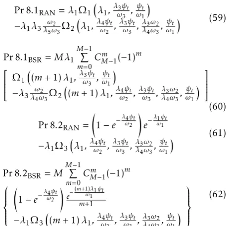
Fig. 2 shows our evaluation and comparison of the performances of the four protocols, i.e., RAN, DR-BSR, NDR-RAN, and NDR-DR-BSR, versus the transmit
power P from -5 dB to 10 dB. We observe that, as
expected, the outage performances of all the protocols are significantly improved when the transmit power
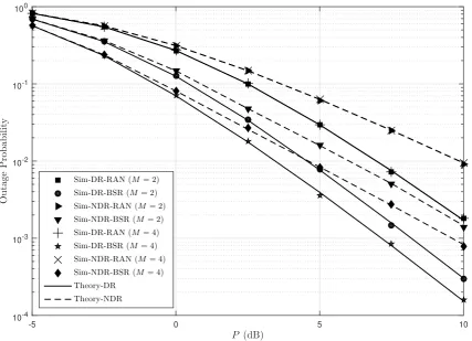
P increases. In Fig. 3, the outage performances of all
protocols are presented versus the power splitting ratio
ρ varying from 0.1 to 0.9. The performances are the
worst when ρ is at 0.1 or 0.9. This phenomenon can
be explained as follows. When ρ= 0.1, the harvested
energy at the best relay in cluster R1 is insignificant;
thus, it is difficult to use that amount of energy to
successfully forward the source data to the destination.
And when ρ= 0.9, the harvested energy is large, but
the decoding performance at the best relay in cluster
R1 is low. Therefore, there is an optimal value ofρthat
balances the decoding performance and the harvested energy at the best relay in cluster R1. For example, the
optimal value of ρ in this scenario is around 0.6; at
this point, the outage performances of all the protocols achieve their best.
We observe in Figs. 2 and 3 that the DR-BSR and NDR-BSR protocols improve in performance when the number of relays is increased in cluster
R1 (M= 2,4) and/or cluster R2 (N = 2,4) due to
increasing the decoding performance and the amount
of harvested energy at the best relay in cluster R1,
and increasing the decoding performance at the best
relay in cluster R2, while the DR-RAN and
NDR-RAN protocols have unchanged performance because the best relay is randomly selected. In addition, as expected, the DR-RAN and DR-BSR protocols achieve higher performance than the NDR-RAN and NDR-BSR, respectively. And the outage performances of the DR-BSR and NDR-DR-BSR protocols are higher than those of the DR-RAN and NDR-RAN, respectively. Thus, we do not show the DR-RAN and NDR-RAN in the next figures. Moreover, we see that the gaps between the
curvesM= 2 andM= 4 of the protocol DR/NDR-BSR
shown in Figure 2 are bigger than those between the
curvesN = 2 andN = 4 in Fig. 3. Therefore, the system
is improved more when we increase the number of
relays in cluster R1 (M) than when we increase the
number of relays in cluster R2 (N). This finding is
shown again in Fig. 6.
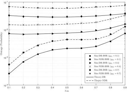
In Fig. 4, the impact of the position of cluster
P (dB)
-5 0 5 10
O
u
tage
Pr
ob
ab
il
it
y
10-4 10-3 10-2 10-1 100
Sim-DR-RAN (M= 2) Sim-DR-BSR (M= 2) Sim-NDR-RAN (M= 2) Sim-NDR-BSR (M= 2) Sim-DR-RAN (M= 4) Sim-DR-BSR (M= 4) Sim-NDR-RAN (M= 4) Sim-NDR-BSR (M= 4) Theory-DR
Theory-NDR
Figure 2. Outage probability versus transmit powerP in dB for the four protocols and forMof 2 and 4 with(xR1, yR1) = (0.5,0.3),
(xR2, yR2) = (0.5,−0.3),ψt= 1bit/s/Hz,ρ= 0.5,η= 0.5, and N = 2.
observed that the outage performance is the worst when
the cluster R1 is farthest away from the source and
destination (yR1= 0.7), and it changes very slightly
when xR1 is changed from 0.1 to 0.9. This can be
explained as follows. When yR1= 0.7, for all values
of xR1 from 0.1 to 0.9, the distances from the source
to cluster R1 and from the destination to cluster
R1 are relatively long, so the decoding performance
and energy harvesting of the link from S to cluster
R1, as well as the decoding performance of the link
from cluster R1 to D, are too low. In this case,
successful transmission occurs almost via the linksS−
D andS−clusterR2−D; hence, the outage performance
changes slightly as xR1 changes. When cluster R1 is
positioned nearer to the source and destination, e.g.,
yR1= 0.4, the outage performances of the DR-BSR and
NDR-BSR increases. As cluster R1 continues moving
nearer (yR1= 0.1), their outage performances continue
to improve. Additionally, there is a big change in the
outage performance when xR1 changes. For instance,
the outage performance is the best when xR1= 0.1
because, at this position, the best relay in cluster R1
can easily decode the source data and harvest enough energy for forwarding the data to the destination.
The performance is decreased significantly whenxR1=
0.9. In addition, the DR-BSR protocol achieves higher
performance than the NDR-BSR protocol for all values
ofxR1andyR1.
Fig. 5 shows the impact of the position of cluster
R2 on the outage performance. As expected, the
DR-BSR protocol outperforms the NDR-DR-BSR protocol for
the same position of clusterR2, and they both achieve
higher performance when cluster R2 is closer to the
source and destination. For example, the performance
when yR2=−0.1 is higher than when yR2=−0.4 and
yR2=−0.7, for all values of xR2. Especially, the two
protocols achieve their highest performances whenxR2
is around 0.7 because this is the optimal position for balancing between decoding the information of the two
linksS−R2 andR2−D.
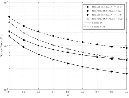
Fig. 6 presents comparisons of the outage
probabili-ties of the DR-BSR and NDR-BSR protocols versusηfor
(M, N) = (2,4) and (M, N) = (4,2). As we can see in Fig.
ρ
0.1 0.2 0.3 0.4 0.5 0.6 0.7 0.8 0.9
O
u
tage
Pr
ob
ab
il
it
y
10-3 10-2 10-1 100
Sim-DR-RAN (N= 2) Sim-DR-BSR (N= 2) Sim-NDR-RAN (N= 2) Sim-NDR-BSR (N= 2) Sim-DR-RAN (N= 4) Sim-DR-BSR (N= 4) Sim-NDR-RAN (N= 4) Sim-NDR-BSR (N= 4) Theory-DR
Theory-NDR
Figure 3. Outage probability versus power splitting ratioρ for the four protocols and forN of 2 and 4 with(xR1, yR1) = (0.5,0.3),
(xR2, yR2) = (0.5,−0.3),P = 5dB,ψt= 1bits/s/Hz,ρ= 0.5,η= 0.5, andM= 2.
protocols in the case of (M, N) = (4,2) is better than in
the case of (M, N) = (2,4). In addition, the effect of the
direct link S−D on the system performance is large.
As we can see, the DR-BSR protocol (considering the
presence of direct linkS−D) gains higher performance
than the NDR-BSR protocol (no direct link S−D) for
both cases of (M, N) = (2,4) and (M, N) = (4,2).
Fur-thermore, as shown in this figure, the outage
perfor-mances of all protocols increase significantly when η
increases, due to increasing the amount of harvested energy as well as the decoding performance at the best
relay in clusterR1.
Fig. 7 presents the outage probabilities of the DR-BSR and NDR-BSR protocols with respect to transmit power
P in dB forψtof 0.3, 0.7, and 1. The performance of the
system is high when the requirement for the outage rate is low, i.e., the outage performances increase when the
target rateψtdecreases.
Finally, as we can see in Figs. 2 to 7, the theoretical results match very well with the simulation results, verifying our derivations in Section 4 and 5.
7. Conclusions
In this paper, we investigate the selection-combining technique at the destination for a system model of a 2-branch cooperative communication system including one energy-constrained relaying branch and one conventional relaying branch. We study two relay-selection schemes (RAN and BSR) for two cases, one with the existence of a direct link (DR) and the other without (NDR) between the source and destination. Thus we considered four protocols: DR-RAN, DR-BSR, NDR-RAN, and NDR-BSR. We derived the closed-form expressions of the outage probabilities for evaluation and comparison of the performances of the four protocols. We derived these theoretical expressions using the Monte Carlo simulation method. From the simulation and theoretical results, we discovered the following. 1) The outage performance of the DR/NDR-RAN protocols do not depend on the number of relays in the two cluster. 2) The DR/NDR-BSR protocols improve the system performance when the number of relays in the two clusters increase; moreover, the system