1 A computational design method for horizontal axis tidal turbines
1 2
ABSTRACT 3
Purpose: A comparative analysis between a straight blade (SB) and a curved caudal-fin tidal 4
turbine blade (CB) is conducted and includes an examination of aspects relating to geometry, 5
turbulence modelling, non-dimensional forces lift and power coefficients. 6
Design/ methodology/ approach: The comparison utilizes results obtained from a default 7
horizontal axis tidal turbine with turbine models available from the literature. A computational 8
design method was then developed and implemented for ‘horizontal axis tidal turbine blade’. 9
Computational fluid dynamics (CFD) results for the blade design are presented in terms of lift 10
coefficient distribution at mid-height blades, power coefficients and blade surface pressure 11
distributions. Moving the CB back towards the SB ensures that the total blade height stays constant 12
for all geometries. A 3D mesh independency study of a ‘straight blade horizontal axis tidal turbine 13
blade’ modelled using CFD was carried out. The grid convergence study was produced by 14
employing two turbulence models, the standard k-ε model and Shear Stress Transport (SST) in 15
ANSYS CFX. Three parameters were investigated: mesh resolution, turbulence model, and power 16
coefficient in the initial CFD, analysis. 17
Findings: It was found that the mesh resolution and the turbulence model affect the power 18
coefficient results. The power coefficients obtained from the standard k-ε model are 15% to 20% 19
lower than the accuracy of the SST model. Further analysis was performed on both the designed 20
blades using ANSYS CFX and SST turbulence model. The variation in pressure distributions yields 21
to the varying lift coefficient distribution across blade spans. The lift coefficient reached its peak 22
between 0.75 to 0.8 of the blade span where the total lift accelerates with increasing pressure before 23
drastically dropping down at 0.9 onwards due to the escalating rotational velocity of the blades. 24
Originality: The work presents a computational design methodological approach that is entirely 25
original. While this numerical method has proven to be accurate and robust for many traditional 26
tidal turbines, it has now been verified further for CB tidal turbines. 27
28
KEYWORDS: 29
Bio-mimicry, Direct Design Method, Horizontal Axis Tidal Turbine, Tidal Energy, Comparative 30 analysis. 31 32 INTRODUCTION 33
Tidal energy is a renewable electricity source that converts the kinetic energy of moving water into 34
mechanical power to drive generators (Shi et al., 2015). This renewable source has minimal CO2 35
emissions and is one of the many sources to address concerns over climate change (Tedds et al., 36
2014). Horizontal axis tidal turbines (HATT) (also known as axial flow turbines) have the rotational 37
axis parallel to the tidal flow and operate in only one flow direction. The mechanical components 38
and principle of HATT operation is similar to the horizontal axis wind turbine (HAWT) – that is, 39
blades are fitted to the hub, a generator converts kinetic energy from the water to mechanical 40
energy, a shaft produces power and a gearbox drives a motor (Bai et al., 2016). 41
42
There have been many advances in the development of the computational power and computational 43
fluid dynamics (CFD) models to simulate the complex flow around the turbine (Malki et al., 2014). 44
Several studies conducted in tidal energy have examined the flow effects around turbines (Divett et 45
al., 2013; Funke et al., 2014; Harrison et al., 2010; Blackmore et al., 2016). For example, the 46
characteristics of a 10m diameter three-bladed HATT and the mesh was generated using ANSYS 47
ICEM CFD (12Chord length x 20Chord length of the airfoils used in the rectangular grid); a very 48
fine mesh near the blade wall region was used to obtain precise results but no y+ values (Goundar 49
and Ahmed, 2013). The authors [ibid] found that by varying the airfoil’s thickness, the blades’ 50
hydrodynamic performance and strength improved, with the rotor producing a maximum efficiency 51
2 experimental data at 15° and 20° of pitch angle and synergized with the previous work of McSherry 53
et al., (2011). The authors [ibid] analyzed the tidal turbine pressure and near-wall effects using 54
shear stress transport (SST) model but also considered the mesh resolution and time step 55
convergence. However, the SST model cannot capture the turbulence 3D effects as the flow passing 56
below the turbine was not modelled by McSherry et al., (2011) (Gayen and Sarkar, 2011; Boris et 57
al., 1992). Subsequently, there are higher 3D turbulence models available which have been 58
rigorously developed and validated against flume tests (Roc et al., 2013; Sescu et al., 2015) but a 59
significant drawback is the computational overhead required to solve the CFD simulation. 60
61
A recent study by Divett et al., (2016) presented a methodical numerical simulation of a large tidal 62
turbine array. Hundreds of layouts were simulated using large eddy simulations (LES) to show the 63
linear relationship between total power capture and its increment as additional rows are added onto 64
turbines. The tidal cycle variation is mainly influenced by astronomical factors i.e. the sun and the 65
moon, and the effects of salinity and temperature stratification are secondary factors (Li et al., 66
2011). Accurately capturing the 3D turbulent flow features of the HATT requires a comprehensive 67
understanding of the physics involved especially when experimental data is missing for validation. 68
Experimental data is expensive to implement and hence, LES provides more flow-physics detail and 69
places less reliance on such data by directly solving the spatially filtered Navier-Stokes equations 70
on the larger turbulent scales (Churchfield et al., 2013; Bin et al., 2013; Ni et al., 2013; Ciri et al., 71
2016). 72
73
This study develops a new computational design methodology for simulating 3D turbulent flow past 74
straight blade (SB) and curved caudal fin blade (CB) HATTs. The design method also conducts a 75
comparative analysis between the prototype blades designed using SST and LES-Smagorisnky 76
turbulence models. The CFD methodology is validated against secondary data available within the 77
literature (Goundar and Ahmed, 2013; Larwood and Zuteck, 2006). By applying this new 78
computational design methodology, the research objective is to augment CFD simulation reliability 79
for the CB tidal turbine blades. 80
81
EXISTING CFD MODELLING IN TIDAL ENERGY CONVERSION 82
Jo et al., (2014) designed a horizontal axis tidal turbine based on the blade element momentum 83
(BEM) method and calculated its efficiency performance to 40%, choosing five as the tip speed 84
ratio. They [ibid] also investigated the wake distribution in the unsteady velocity flow affecting the 85
tidal turbine system. CFD analysis was performed using a SST turbulence model and the curves of 86
power coefficient (CP) and torque generated from the shaft were presented for different velocities. 87
The airfoils were arranged in sequential order with appropriate twist angles and chord lengths to 88
predict the tidal turbine performance using CFD to predict its torque and CP. Kim et al., (2012) 89
analyzed a bi-directional vertical axis turbine performance in a larger area of tidal channel. 90
Hexahedral mesh was applied in the augmentation channel and an SST turbulence model was 91
selected. The tidal turbine blade performance was accessed based on the pressure and lift 92
coefficients, hence demonstrating the two most significant sensitivities that cause cavitation studies 93
at different angles of attack especially for the leading edge. Rocha et al., (2014) carried out a 94
numerical investigation and calibrated a SST turbulence model to test the operational performance 95
of a small scale horizontal axis wind turbine (SS-HAWT). They [ibid] studied aerodynamic 96
performance of the SS-HAWT based on the turbulence intensity and characteristic length (β*) to 97
reveal the varied effects of friction over the blades. 98
99
Afgan et al., (2013) presented a comparison between Reynolds-averaged Navier-Stokes (RANS) 100
models SST and LES numerical solutions for a three bladed HATT, validating the implemented 101
sliding mesh technique for the unstructured mesh code over a range of tip speed ratios (TSRs). The 102
LES solver’s accuracy was tested against the optimum design condition to investigate the wake and 103
3 al., (2013) compared three different CFD modelling approaches on a vertical axis wind turbine in 105
higher angles of attack. The NACA 0018 SB foil was simulated using LES with a high angle of 106
attack flow. In symmetrical airfoils the stall angles appear between 10° to 15°. The authors [ibid] 107
also commented on the SST turbulence model’s efficacy and considered it to be assuring when 108
simulating the adverse pressure gradients in incompressible flow. However, when SST was 109
compared to LES, LES was computationally more challenging but produced more realistic 3D 110
vortex diffusion and flow separation in unsteady flow computations. Force coefficients were 111
calculated in the span wise distribution of the airfoil blades, thus proving LES as a better high 112
fidelity CFD modelling technique. Kang et al., (2012) simulated 3D turbulent flow around an axial 113
tidal turbine, placed on the rectangular bed comprising an open channel accommodating the CFD 114
domain to carry out LES simulations. The convoluted turbine geometry comprising rotor and stator 115
components with moving boundaries were managed by engaging the curvilinear immersed 116
boundary method. The CFD simulations were compared to the marine hydropower turbine using 117
systematic grid refinement and calculating the torque sensitivity analysis. The simulations 118
indicated that pressure fields near the turbine blades generated torque and extracted power from the 119
water column. 120
121
The extant literature reveals that the SST model is the most popular turbulence model used in steady 122
state analysis of tidal turbine blades and LES for transient simulations in the absence of 123
experimental data for validation. The literature also illustrates the need for new and alternative/ 124
innovative methodological approaches for the CB design. 125
126
A COMPUTATIONAL DESIGN METHODOLOGY 127
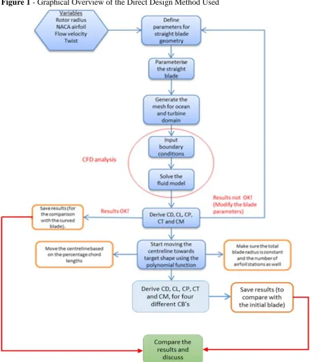
The direct design method represents an optimized approach to product design that requires an 128
understanding of the problem before collecting numerical data for analysis, validation or 129
verification using mathematical modelling (Campi et al., 2002; Shi et al., 2012; Liu, 2010; Wang et 130
al., 2012; Thapar et al., 2011). The direct design method begins by modelling the parametric three-131
dimensional SB, and then a rectangular mesh domain is generated for inputting the boundary 132
conditions. After defining the boundary conditions, CFD analysis (as a prominent mathematical 133
modelling technique) is performed on the tidal turbine rotors, the numerical results are compared 134
with existing data in the literature. The final step builds the three dimensional model (Figure 1), 135
where chosen turbulence models are tested and verified by further investigation to allow emergence 136
of new data (Hudgins and Lavelle, 1995) The CFD results collected from the SB were 137
comparatively analysed and evaluated with the curved caudal fin shaped blades. 138
139
<Insert Figure 1 about here> 140
141
The end objectives of the chosen direct blade design method were to: compare the highest power 142
coefficient obtained for the CB with data available within tidal turbine blade literature. 143
144
Design of the SB HATT 145
146
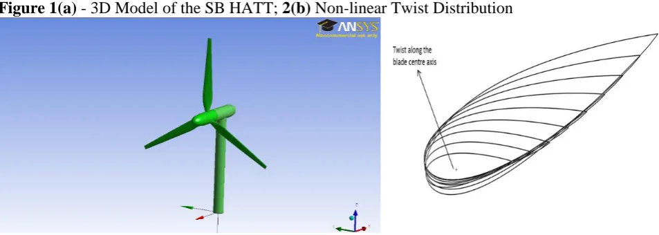
The SB HATT was designed in ANSYS Design Modeller (refer to Figures 2a; 2b). The airfoil 147
considered for all the horizontal blades is a symmetrical NACA 0018. The spanwise distribution of 148
the airfoils are stationed at every 10% of the blade whilst the distance between hub circle and the 149
root airfoil is 20% of the total blade height. 150
151
<Insert Figures 2a and b about here> 152
153
The blade hub is circular and its diameter is 40% of the root airfoil chord length. The blade twist 154
angle is higher at the root airfoil because it experiences less rotational forces and it gradually 155
4 157
<Insert Table 1 about here> 158
159
Design of the CB 160
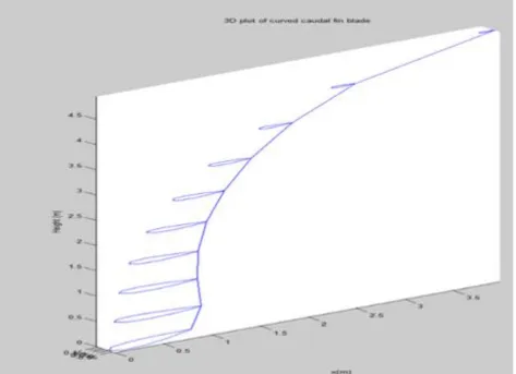
The 3D curved set of centroids defines the shape of the CB. A predictive MATLAB program was 161
created in which the centroids of the NACA airfoil centres form a 3D shape (refer to Figure 3). The 162
MATLAB program computes the centre of mass (gravity) for the set of airfoils used in modelling 163
the CB. 164
165
<Insert Figure 3 about here> 166
167
The weighted centroid uses the pixel intensities in the airfoil region which weights the centroid 168
calculation and the twist angle, which acts as the function of the incremental blade length, is further 169
modified to create a smooth twist by fitting a third order polynomial function. The initial values of 170
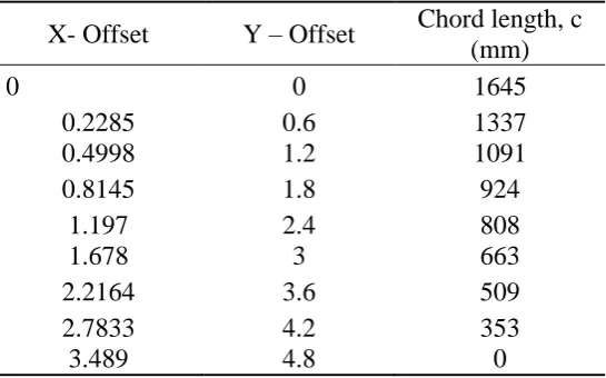
the CB NACA profile chord lengths are defined in Table 2 whilst the default profile chosen is 171
NACA 0018. 172
173
<Insert Table 2 about here> 174
175
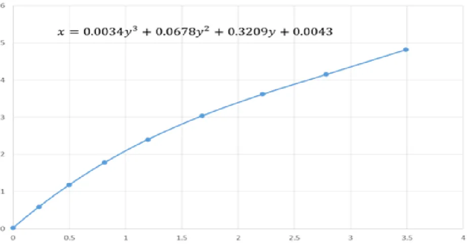
The X-offset and Y-offset values are used to construct the skeletal (centre line) of the CB. For 176
programming purposes, the nearest third order polynomial regression equation on the centre line 177
curve (refer to Figure 4) is defined as: 178
179
<Insert Figure 4 about here> 180
181
Each NACA profile centre is built on the centre line which acts as a master and each profile datum 182
sits along its length divided by the height - the numbers of stations stay constant to reduce the 183
computational overhead. The NACA profile sections of the curved blade are considered parallel to 184
the x-axis, that is, the normal of each NACA section should be the y-axis. The skeleton which is 185
fitted on the midpoint of the each airfoil has a decrease in the chord length in the blade spanwise 186
direction which increases the surface area of the CB. The third order polynomial is fitted on the 187
skeleton of the caudal fin centerline, starting at the airfoil root centre and passing through all the 188
airfoil stations to the tip of the airfoil; at this end of the blade, bending occurs to create the CB. The 189
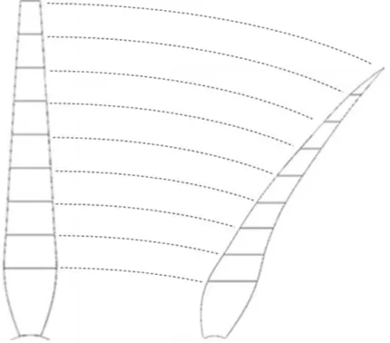
chord lengths of the SB can be varied in linear or non-linear progression along the span-wise 190
direction to reach the CB (refer to Figure 5). 191
192
<Insert Figure 5 about here> 193
194
Strategy to Move the Curved Blade Shape Backwards to SB Shape
195
The polynomial centre-line from the root chord was moved in the percentage chord lengths in order 196
to reach the target shape. For the initial experimentation, the percentage chord lengths were moved 197
in 0%, 25%, 50%, 75%, and 100% increments; where 0% represents the initial SB chord lengths. 198
For convenience during experimentation, the same blade is simulated whilst the total blade height 199
and number of stations are kept constant until the best design is found (i.e. maximum power 200
coefficient of the blade system). The tidal turbine blade power coefficient is predominantly 201
sensitive to total blade height but also blade twist and chord length distribution - changing the value 202
of each and every design variable would be time consuming. To overcome this problem, repetitive 203
transformations of the default blade design method was used. Using this approach, the percentage 204
based chord lengths were selected and the third order polynomial function remains constant 205
ensuring that the blade span or total blade height will replicate the default SB. Thus it was possible 206
to define a design study strategy that moved the target shaped CB backwards to the SB shape using 207
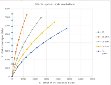
5 209 𝑻𝑨𝑺𝑻𝑵 = 𝑻𝑺𝑿𝑪 × ( 𝑹𝑷 𝟏𝟎𝟎) Equation 1
Where: TASTN is the required airfoil station value; TSXC is the target shape X-coordinate value for 210
the particular airfoil station; and 𝑅𝑝 is the required chord length percentage. After calculating the X 211
and Y-offsets for the blade spinal axis variation, the backward design strategy can be plotted in 212
Figure 6. 213
214
<Insert Figure 6 about here> 215
216
A COMPARATIVE ANALYSIS BETWEEN THE FIVE DESIGNED PROTOTYPE 217
BLADES 218
Figure 7 illustrates the rectangular computational grid which was used to model the seawater 219
domain and the turbine disc domain, for the SB and CB geometries. The seawater domain extends 220
five times the turbine diameter at the inlet, ten times of the turbine diameter at the outlet whilst the 221
height of the rectangular grid is five times of the turbine diameter. The turbine domain was 222
designed as a rotating domain in CFX and then a full 360° mesh surrounding the tidal turbine 223
blades. Figure 7 shows blade automated meshing including the hub and tips of the SB and the CB. 224
225
<Insert Figure 7 about here> 226
227
Mesh Independency study 228
To establish the accuracy of the CFD solution, and to keep the computational costs low, the straight 229
blade was analysed using: the standard k-ε model, and SST model, at uniform Vin = 2.5m/s, and λ = 230
5. The grid convergence study was performed by developing three different meshes: with a coarse, 231
medium, and fine grid for all six different meshes of the Straight Blade to predict the power, lift 232
coefficients, and torque on normalised mesh cells to determine how the mesh quality affects CFD 233
simulation results. 234
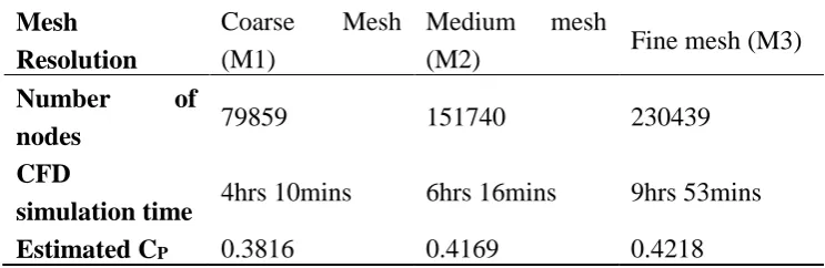
The number of nodes and the simulation time for the three cases simulated using the SST model are 235
highlighted in Table 3, and the three cases simulated using the standard k-ε model are given in 236
Table 4. Table 3, and 4 summarise the key characteristics of the meshes, and it is very clear that 237
CFD simulation time is highly dependent on the number of mesh nodes considered. The six meshes 238
generated have near wall resolution i.e. y+ < 10 by using the standard wall function approach to 239
avoid unsatisfactory results when using the standard k – ε model. 240
241
<Insert Table 3 about here> 242
243
<Insert Table 4 about here> 244
245
In the case of the investigated meshes of the straight blade, the turbine domain has an increased 246
mesh resolution. The mesh is refined in the grids from M1 to M6 where M1, M2, M3 represent 247
coarse, medium, and fine mesh generated for the SST turbulence model; and M4, M5, M6 248
represent coarse, medium, and fine mesh generated for the standard k-ε turbulence model. The 249
estimated power coefficient increased from 0.2271 to 0.4218 as shown in Figure 8. 250
251
<Insert Figure 8 about here> 252
253
It is important to note that the mesh resolution plays a pivotal role in the final CFD results. The 254
mesh nodes need to be small to resolve the boundary layer on the blade surfaces. The highest CP 255
6 account for nearly 1% difference in the estimated power coefficients, but the final CFD simulation 257
time required for convergence of the two meshes has a significant difference when the conventional 258
mesh independency method is employed. The power coefficients obtained from the standard k-ε 259
model are almost 15% to 20% lower than the SST model power coefficients, which is due to the 260
poor performance of the k-ε model in near-wall regions and in adverse pressure gradients i.e. the 261
fluid flow near the turbine blade surfaces; which causes the k-ε model to underestimate the power 262
coefficient. 263
264
It is clear from the final CFD simulation results that the simulation time is highly dependent on the 265
number of mesh nodes, and the turbulence model selected. As shown in Figure 8 when using k-ε 266
model for all the meshes (M4, M5, and M6) employed the CFD solution under predicts power 267
coefficient when compared with the SST model. M1 leads to the reasonable prediction of the power 268
coefficient on the straight blade, whereas the power coefficient of M3 is slightly better than M2. 269
Due to the slight difference, medium mesh (M2) is best regarding computational costs and is further 270
employed for the numerical analysis carried out in the following section of the turbulence model 271
comparison study. 272
273
Turbulence model comparison study
274
To understand the sensitivity of the CFD solution a consecutive study was carried out with these 275
turbulence models at medium sized meshes. From the mesh dependency test conducted it has been 276
found that the SST model performs superiorly in adverse pressure gradient situations than the 277
standard k-ε model; because SST model is a unification of k-ε model and k-ω model for free stream 278
and inner boundary layer problems respectively. Figure 9 shows the torque coefficient related to 279
each of the two turbulence models analysed for the medium mesh. As shown in Figure 9 the SST 280
model medium mesh has higher CM than the standard k-ε model in all the nine different TSR’s. It 281
can also be seen that the torque coefficient of SST medium mesh model increased by more than 282
25% when compared to the standard k-ε model medium mesh. 283
284
<Insert Figure 9 about here> 285
286
The highest CM is achieved at λ= 5 for both the cases, CM increases with the increasing TSR and 287
acts as a function of TSR. It can also be noted that the non-linearity in the torque coefficient occurs 288
after TSR of 5, and the k-ε model fails to capture this, due to the boundary layer and turbulence 289
quantities to the blade wall. 290
291
Figure 10 shows that the power coefficient increases steadily until TSR ≈ 5, at which it shows the 292
peak CP ≈ 0.4169 for the SST model medium mesh; after which it shows a drastic reduction with 293
the increasing λ > 6. The curve for medium mesh the k-ε model shows that it predicts a lower power 294
coefficient to a satisfying level of accuracy, and also under predicts the values with increasing λ. 295
However, the numerical CP prediction by medium mesh the SST model observed values are 296
approximately 20% higher than medium mesh the k-ε model simulation, the range 5 ≤ λ ≤ 6 was 297
also validated (Bahaj et al., 2007; McSherry et al., 2011); and considered to be optimum range for 298
HATT. The standard k-ε model is incapable of capturing the account of rotational forces and their 299
effects on the turbine blades, and due to the near wall physics implementation. Thus the CP 300
prediction by SST model is more acceptable when compared to the power coefficient predictions by 301
the standard k-ε model. 302
303
<Insert Figure 10 about here> 304
305
As a result of the mesh independency test conducted it can be concluded that the overall power 306
coefficient shown by the SST turbulence model is more reasonable than the standard k-ε model, for 307
7 not employed in any further CFD tests conducted in this research. The power coefficient of a HATT 309
is highly sensitive to the turbulence model chosen for the CFD analysis; however the mesh 310
independent CFD solution for SST medium mesh satisfactorily achieves the mesh independency 311
over the SST fine mesh solution which requires a massive computational overhead. Hence, the 312
medium mesh is used to conduct the steady state analysis in following sections. 313
314
Steady state CFD analysis 315
The steady state simulations were conducted using ANSYS CFX via the SST turbulence model. In 316
ANSYS CFX, the pressure-velocity coupling was achieved using the Rhie - Chow Option, and all 317
the interpolation and advection values were set at high resolution. In the meshing aspect, some 318
controls were modified to suit the concentration on the curved shaped blades because of the 319
additional bend on the surface. Table 5 summaries the blade model functions and the respective 320
characteristics. 321
322
<Insert Table 5 about here> 323
324
Table 3 illustrates that the number of nodes of the CB 100% case study are almost twice that of the 325
SB case study – this is due to the flow being considerably complicated and the blade surfaces being 326
bent for the curved blade shape. The three-dimensional modelling and steady state CFD simulations 327
presented are conducted at constant inlet velocity of 2.5m/s, using high turbulence intensity of 10%. 328
The outlet pressure was defined as 0bar, the blade was defined as a rotating wall, with no slip wall 329
condition for mass and momentum option. The bottom and side walls were defined as free slip 330
walls to incorporate accuracy when solving the continuity equation. The front and back walls were 331
defined as inlet and outlet walls respectively. As the seawater flow velocity progressed over the 332
blade pressure side, the pressure increased especially on the tip of the blade where rotational 333
velocity was at its highest point. Figure 11 shows the comparison of the blade pressure distribution 334
on the case studies performed (blades rotate anti-clockwise). 335
336
<Insert Figure 11 about here> 337
338
Data accompanying Figure 11 compares the steady-state pressure distribution on the five blade 339
designs. Numerical simulations show how the seawater flow behaves on the trailing and leading 340
edges on the pressure side of the blade. The varying lift coefficient distribution is also demonstrated 341
by plotting the blade mid-span coefficient of lift distributions for all five blade designs. CB 75% 342
shows the highest lift coefficient at 0.5 blade span location with a peak value of 0.182 while CB 343
100% shows the lowest lift coefficient value of 0.0835 amongst all the blades designed. 344
Interestingly, Figures 11 and 12 illustrate that the pressure is higher on the outer radius of trailing 345
edge of the CB 100% (target shape blade), as compared to the other four blade geometries. This 346
may be because the target shape is modelled as an assumption of the fish caudal fin and generates 347
flow reattachment. Pressure near the tip region of all five designs increases as compared to the rest 348
of the blade and the leading edge contributes to the pressure distribution increase on the pressure 349
side. Simultaneously, the trailing edge causes negative pressure distribution increase on the suction 350
side which contributes to lift force decrement and torque force reduction. 351
352
<Insert Figure 12 about here> 353
354
Figure 12 illustrates that variations in the pressure distribution yield the varying lift coefficient 355
distribution on the airfoil chord length. The lift coefficient increases with the increase in blade span 356
until 0.8 blade span location, after which a drastic reduction near the blade tip occurs. Although the 357
lift coefficient varies in magnitude for all the blade designs, it can be observed that the CB 100% 358
results in lower lift coefficients when compared to the other four blade designs. Therefore, it can be 359
8 drag increase. This would cause torque reduction, leading to a lower power coefficient as the bend 361
on the blade increases. 362
363
Transient CFD analysis 364
Transient simulations for the five blade designs were generated using the LES-Smagorinsky sub-365
grid scale model and fine unstructured mesh in an integrated time step. For all five design LES 366
cases, the time step used for the simulation required for the flow to pass entirely through the turbine 367
was about 0.15million time steps. The time step size for each case was set to 3 x 10⁻⁵ which 368
coincides with approximately ten blade rotations for the TSR = five for all five cases, which is 369
equivalent to 4.89 x 10⁵ seconds or 135.83 hours. Multiple frames of reference (MFR) was applied 370
to the turbine disc analysis as it was a rotating domain based on the general grid interface (GGI) 371
available in CFX. The turbulence intensity at the inlet of the computational domain was defined as 372
15% (typical seawater value) and as the tidal turbine blade geometry is a high turbulence intensity 373
case. It should be noted that the non-uniform velocity of 2.5 m/s was applied to all five blade 374
designs. The turbulence intensity gradually decreased at a distance of four rotor diameters 375
downstream from the inlet to 13.68% due to velocity instability, and the turbulence level at the rotor 376
leading edge was observed to be 12.82%. This gradual decrease was expected due to the higher 377
rotational velocity of the blades which correspond to the blade tip. At the solid boundaries (blade 378
geometry) the near wall node was y+ = 50 < y+ < 300 (Piomelli and Balaras, 2002; Tessicini and 379
Leschziner, 2007) because of the two zonal layer LES approach used and the refined fine mesh in 380
the tidal turbine domain was embedded into the ocean flow domain. The mesh parameter values for 381
LES- Smagorinsky simulations are reproduced in Table 6. 382
383
<Insert Table 6 about here> 384
385
The residuals convergence criterion for each time step was set to 10−5 and two monitors were used 386
namely (Oberkampf et al., 2004; Lim et al., 2012; Versteeg and Malalasekera, 2007): 387
388
Scaled residual monitors for mass and momentum of the iterative process; and 389
Lift coefficient CL trend as a function of the iteration number for LES-Smagorinsky solution. 390
The CFD solution is considered to have converged when the mass and momentum residuals present 391
a constant trend under 10−5 value which is illustrated in Figure 13 where the residuals represent the 392
downward trend of the scaled residuals for the CB 75% LES-Smagorinsky solution. 393
394
<Insert Figure 13 about here> 395
396
Figure 13 illustrates that the residuals mark the continual removal of the unwanted imbalances 397
thereby causing the CFD iterative process to converge rather than diverge. The mass residual at the 398
time step number 1795 reached the convergence value of 7.269e-06 and 9.51e-06 on the time step 399
2665 when the transient solution was stopped. The discretised mass and momentum equations are 400
presumed to be converged when they reached the convergence criterion and did not change with 401
further iterations. The mass flow balance between the inlet and outlet were also verified for all the 402
transient CFD simulations performed to ensure continuity of the solution (CFX-Solver Theory 403
Guide, 2009; Oberkampf and Trucano, 2000). The lift coefficient (CL) history over iterations was 404
also monitored to check the unsteady convergence of the LES-Smagorinsky solution (refer to 405
Figure 14 for CB 75%). There was no appreciable change observed in the lift coefficient after 1100 406
timesteps but the solution was still monitored for more than 1500 time steps as the lift coefficient 407
elevations to the fixed value of 0.1795. 408
409
<Insert Figure 14 about here> 410
9 LES transient simulations conducted sought to compare the results obtained with the steady state 412
SST simulations. The turbine pressure contours (LES-Smagorinsky) (Figure 15) illustrate that a 413
difference between the pressure and suction sides of the blade becomes smaller as the rotational 414
velocity increases on the upper part of the blade. In comparison to steady state simulations, this 415
increases the net lift and torque. 416
417
<Insert Figure 15 about here> 418
419
The pressure prediction on the tip of the blade (where the rotational velocity of the blade is at its 420
highest) also causes higher lift on the pressure side of the blade. Figure 16 reveals that lift 421
distribution on the suction side of the mid-height is larger than on the pressure side of the airfoil. 422
This scenario significantly increases drag force on the CB 100% (target shape) as compared to the 423
other four geometries, making it directly proportional to the bend on the blade. It also illustrates that 424
the most affected region by the seawater is the tip chord of the blade along leading and trailing 425
edges. The drag increment for the CB 100% was expected seeing the negative pressure on the 426
suction side on the tip, proving to generate cavitation in extreme velocity conditions. 427
428
<Insert Figure 16 about here> 429
430
The LES simulations demonstrate that the kinetic energy contained in the seawater flow is extracted 431
from the blade’s upper stream and that pressure prediction is more realistic as there is no flow 432
divergence in real life HATT’s. The prediction of the lift caused due to the large separation of the 433
flow and the pressure surface of the blades consequently increases the predicted power coefficients, 434
and causes less discrepancy in the vorticity of the pressure field. Interestingly, LES solutions with a 435
high computational overhead demonstrate a clear phenomenon of the pressure changes on the blade 436
and avoids over prediction of the lift and power coefficient. 437
438
DISCUSSION OF THE COMPARISON BETWEEN THE DESIGNED BLADES 439
The performance of SST and LES-Smagorinsky turbulence models are examined by plotting the lift 440
coefficient against various angles of attack (refer to Figure 17). There is a gradual decrease in the 441
lift coefficient after the six degrees of angle of attack for all the cases, as the flow becomes highly 442
non-linear and the rotational velocity of the blades reaches its maximum. The mass flow rate of the 443
seawater is a function of the cross-sectional area of the turbine blades and its velocity, therefore the 444
bend on the curved blades makes the mass flow rate drop the lift coefficient after 6 degrees of angle 445
of attack. 446
447
<Insert Figure 17 about here> 448
Therefore, it can be concluded that with the increase in the angle of attack the turbine blades would 449
rotate faster but simultaneously kinetic energy available in the seawater exerts a drag force upon the 450
blade, causing a reduction of the overall power coefficient of the turbine blade. The output power 451
notably depends on the inlet seawater velocity (refer to Figure 18). Although the CB 100% yields 452
almost 15% more power than the SB in case of all the flow velocities, this does not necessarily 453
mean that it would yield the highest power coefficient for the designed blades. 454
455
<Insert Figure 18 about here> 456
457
The SB produces 366 kW of power and a power coefficient of 0.4028, whilst the CB 100% 458
provides approximately 20% more output power than the SB, and about 15% more power than the 459
most efficient CB 75%. However, the power coefficient for the target shape blade i.e. CB 100% is 460
0.3951 and 0.3728 for the SST and LES-Smagorinsky CFD simulations respectively. As 80% of 461
turbine blade efficiency (i.e. the power coefficient) is generated from the midsection of the designed 462
10 the SST and the LES-Smagorinsky CFD tests. There was little difference between the results from 464
the LES-Smagorinsky CFD simulations but these results confirm the accuracy of the comparative 465
analysis while using two different turbulence modelling techniques. Therefore, the CB 75% will be 466
put forward to allow the coefficient power comparison with the standard (suitable) HATT models 467
available in the tidal turbine literature. 468
Goundar and Ahmed (2013) designed a three bladed 10m diameter HATT, and achieved a 469
maximum efficiency of 47.5% with a power output of 150kW, for the constant seawater velocity of 470
2m/s. The CB 75% is also three bladed and has a 14.2 diameter, and yields an efficiency of 51.78% 471
for LES simulations with a power output of 435kW; which is higher than the overall efficiency 472
achieved by Goundar and Ahmed [9]. At the same time the benefit of designing a blade like a CB 473
generates higher lift and power coefficients at lower and higher tidal current velocities, and this has 474
been demonstrated with the CFD simulations presented above. The STAR blade to generate low-475
cost electricity from wind designed by Larwood & Zuteck (2006) implements swept blade design 476
parameters and produces annual power output which ranges from 1.5 to 3MW. The designed 477
turbine blades are 71 to 126m in diameter and have rated generator speed of 1800rpm, and the 478
designed swept wind turbines produce 10 to 15% more power than the standard wind turbines 479
available in the current market. A direct comparison between the results obtained from this research 480
with the STAR blade is beyond the scope of this research, as the maximum diameter a tidal turbine 481
can have 22m (Bahaj et al., 2007; Bahaj et al., 2007; Batten et al., 2008), and as the designed CB 482
75% is 14.4m in diameter. A general comparison of the annual power output can be made, i.e. 483
designing the curved caudal fin blades produces at least 10% more annual power output than the 484
standard straight blades which has been shown by both the studies i.e. by this research and by 485
Larwood & Zuteck (2006). 486
In summary, analysis results confirms that bio-mimicking the caudal fin look-alike turbine blade 487
i.e. CB 75%, produces greater efficiency than the default SB which was designed according to the 488
tidal turbine blade literature and meets the aim of this paper. 489
490
CONCLUSIONS 491
It can be concluded that although LES-Smagorinsky provides a better result than the SST 492
simulations, it also has a massive computational overhead. The CFD results allow a further 493
comparison of the power coefficients; proving that a CB produces more efficiency than the standard 494
HATT’s at lower and higher tidal current velocities. The most fundamental challenge confronting 495
this research was to validate the CFD methodology for the case studies performed with real world 496
data. This is also the most significant problem faced in the wind turbine industry, to which this 497
research could contribute. To overcome this challenge, a comparative analysis was performed for 498
the SB and CB 75% with the tidal turbine literature which thus helps the future tidal turbine blade 499
designers in knowledge transfer, particularly on turbulence model selection. A mesh independency 500
study of a straight blade to determine the mesh sensitivity and its effects on the CFD simulation 501
results. The grid convergence study was simulated using two turbulence models: the standard k-ε 502
model, and SST turbulence model at coarse, medium, and fine mesh resolution thus simulating six 503
different mesh sizes. This paper has shown that obtaining mesh independent solutions is a 504
fundamental need for all the tidal turbine blade designers due to the sensitivity of the lift coefficient 505
of the tidal turbine. 506
507
The standard k-ε model under predicts the power coefficients and the simulation time is highly 508
dependent on the mesh and turbulence model chose for CFD analysis. The highest CP obtained 509
from the mesh independent study conducted is 0.4218 for M3 from SST model and the lowest CP 510
0.2693 for M6 using k-ε model. M2 and M3 account for nearly 1% difference in the estimated 511
power coefficients, but the final CFD simulation time required for convergence of the two meshes is 512
substantially different when conventional mesh independency method is employed. Pressure 513
distribution is a predominant output for determining the lift, and power coefficients, and also to 514
11 trend of the peak lift coefficient being observed at 0.75 to 0.8 of the total blade span before 516
drastically dropping down at 0.9 onwards due to the increasing rotational velocity of the blades. 517
518
The unsteady convergence is an iterative process of the transient solution which needs to be 519
monitored to calculate the accuracy of the transient CFD solution. This was done by monitoring the 520
scaled residuals for mass, and momentum and observing lift coefficient as a function of the 521
iteration. The removal of unwanted imbalances over time steps result in the CFD solution to 522
converge and do not change with further iterations. Future work derived from the observations 523
made from this research should seek to develop a design automation closed loop system using 524
Knowledge Based Engineering (KBE) principles to design a robust tidal turbine blade design which 525
would be optimal throughout the year. The designed closed loop system would automatically 526
parameterize blade geometry, generate automatic mesh, and the numerical results by itself. 527
12 REFERENCES
529
Afgan I, McNaughton J, Rolfo S, Apsley DD, Stallard T, Stansby P. (2013) Turbulent flow and 530
loading on a tidal stream turbine by LES and RANS. International Journal of Heat and Fluid 531
Flow. Vol. 43, pp. 96–108. 532
ANSYS INC. CFX-Solver Theory Guide 2009. 533
Bahaj AS, Batten WMJ, McCann G. (2007) Experimental verifications of numerical predictions for 534
the hydrodynamic performance of horizontal axis marine current turbines. Renewable Energy. 535
Vol. 32, pp. 2479–90. 536
Bahaj AS, Molland AF, Chaplin JR, Batten WMJ. (2007) Power and thrust measurements of marine 537
current turbines under various hydrodynamic flow conditions in a cavitation tunnel and a towing 538
tank. Renewable Energy. Vol.32, pp. 407–26. 539
Bai G, Li W, Chang H, Li G. (2016) The effect of tidal current directions on the optimal design and 540
hydrodynamic performance of a three-turbine system. Renewable Energy. Vol. 94, pp. 48–54. 541
Batten WMJ, Bahaj AS, Molland AF, Chaplin JR. (2008)The prediction of the hydrodynamic 542
performance of marine current turbines. Renewable Energy. Vol. 33, pp. 1085–96. 543
Bin JI, LUO X, PENG X, WU Y. (2013) Three-dimensional large eddy simulation and vorticity 544
analysis of unsteady cavitating flow around a twisted hydrofoil. Journal of Hydrodynamics. 545
Vol.25, pp. 510–9. 546
Blackmore T, Myers LE, Bahaj AS. (2016) Effects of turbulence on tidal turbines: Implications to 547
performance, blade loads, and condition monitoring. International Journal of Marine Energy. 548
Vol. 14, pp. 1–26. 549
Boris JP, Grinstein FF, Oran ES, Kolbe RL. (1992) New insights into large eddy simulation. Fluid 550
Dynamics Research. Vol. 10, pp. 199–228. 551
Campi MC, Lecchini A, Savaresi SM. (2002) Virtual reference feedback tuning: a direct method 552
for the design of feedback controllers. Automatica. Vol.38, pp. 1337–46. 553
Churchfield MJ, Li Y, Moriarty PJ. (2013) A large-eddy simulation study of wake propagation and 554
power production in an array of tidal-current turbines. Philos Trans R Soc London A Math Phys 555
Eng Sci. Vol. 371:20120421 556
Ciri U, Rotea M, Santoni C, Leonardi S. (2016) Large Eddy Simulation for an array of turbines with 557
Extremum Seeking Control. American Control Conference, Boston, MA, USA, pp. 531–6. 558
Divett T, Vennell R, Stevens C. (2013) Optimization of multiple turbine arrays in a channel with 559
tidally reversing flow by numerical modelling with adaptive mesh. Phil Trans R Soc A. Vol. 560
371, 20120251. 561
Divett T, Vennell R, Stevens C. (2016) Channel-scale optimisation and tuning of large tidal turbine 562
arrays using LES with adaptive mesh. Renewable Energy. Vol. 86, pp. 1394–405 563
Funke SW, Farrell PE, Piggott MD. (2014) Tidal turbine array optimisation using the adjoint 564
approach. Renewable Energy. Vol. 63, pp. 658–73. 565
Gayen B, Sarkar S. (2011) Direct and large-eddy simulations of internal tide generation at a near-566
critical slope. Journal of Fluid Mechanics. Vol. 681 pp. 48–79. 567
Goundar JN, Ahmed MR. (2013) Design of a horizontal axis tidal current turbine. Applied Energy. 568
Vol. 111, pp. 161–74. 569
Harrison ME, Batten WMJ, Myers LE, Bahaj AS. (2010) Comparison between CFD simulations 570
and experiments for predicting the far wake of horizontal axis tidal turbines. IET Renewable 571
Power Genereration. Vol. 4, pp. 613–27. 572
Hudgins DW, Lavelle JP. (1995) Risk management in design engineering bids. University of North 573
Texas Libraries, Digital Library, Kansas City, Missouri. 574
Jo C-H, Lee J-H, Rho Y-H, Lee K-H. (2014) Performance analysis of a HAT tidal current turbine 575
and wake flow characteristics. Renewable Energy. Vol. 65, pp. 175–82 576
Kang S, Borazjani I, Colby JA, Sotiropoulos F. (2012) Numerical simulation of 3D flow past a real-577
life marine hydrokinetic turbine. Advances in Water Resources. Vol. 39, pp. 33–43. 578
Kim K-P, Ahmed MR, Lee Y-H. (2012) Efficiency improvement of a tidal current turbine utilizing 579
13 Larwood S, Zuteck M. (2006) Swept wind turbine blade aeroelastic modeling for loads and 581
dynamic behavior. AWEA Wind. pp. 1–17. 582
Li C, Zhu S, Xu Y, Xiao Y. (2013) 2.5 D large eddy simulation of vertical axis wind turbine in 583
consideration of high angle of attack flow. Renewable Energy. Vol. 51, pp. 317–30. 584
Li M, Radhakrishnan S, Piomelli U, Rockwell Geyer W. (2010) Large-eddy simulation of the tidal-585
cycle variations of an estuarine boundary layer. Journal of Geophysical Research Ocean. Vol. 586
115. 587
Liu P. (2010) A computational hydrodynamics method for horizontal axis turbine--Panel method 588
modeling migration from propulsion to turbine energy. Energy. Vol. 35, pp. 2843–51. 589
Malki R, Masters I, Williams AJ, Croft TN. (2014) Planning tidal stream turbine array layouts using 590
a coupled blade element momentum--computational fluid dynamics model. Renewable Energy. 591
Vol. 63, pp. 46–54. 592
McSherry R, Grimwade J, Jones I, Mathias S, Wells A, Mateus A. (2011) 3D CFD modelling of 593
tidal turbine performance with validation against laboratory experiments. 9th European Wave 594
Tidal Energy Conference, University of Southampton, UK. 595
Mo J-O, Choudhry A, Arjomandi M, Lee Y-H. Large eddy simulation of the wind turbine wake 596
characteristics in the numerical wind tunnel model. Journal of Wind Engineering and Industrial 597
Aerodynamics. Vol. 112, pp. 11–24. 598
Oberkampf WL, Trucano TG, Hirsch C. (2004) Verification, validation, and predictive capability in 599
computational engineering and physics. Applied Mechanics Reviews. Vol. 57, pp. 345–84. 600
Oberkampf WL, Trucano TG. (2000) Validation methodology in computational fluid dynamics. 601
Fluids 2000 Conference and Exhibit Denver,CO,U.S.A. pp. 19–22. 602
Piomelli U, Balaras E. (2002) Wall-layer models for large-eddy simulations. Annual Reviews in 603
Fluid Mechanics. Vol. 34, pp. 349–74. 604
Roc T, Conley DC, Greaves D. (2013) Methodology for tidal turbine representation in ocean 605
circulation model. Renewable Energy. Vol. 51, pp. 448–64. 606
Rocha PAC, Rocha HHB, Carneiro FOM, da Silva MEV, Bueno AV. (2014) k-ω SST (shear stress 607
transport) turbulence model calibration: A case study on a small scale horizontal axis wind 608
turbine. Energy. Vol. 65. pp. 412–8. 609
Sescu A, Meneveau C. (2015) Large-Eddy Simulation and Single-Column Modeling of Thermally 610
Stratified Wind Turbine Arrays for Fully Developed, Stationary Atmospheric Conditions. 611
Journal of Atmospheric and Oceanic Technology. Vol. 32, pp. 1144–62. 612
Shen H, Li S, Chen G. (2012) Quantitative analysis of surface deflections in the automobile exterior 613
panel based on a curvature-deviation method. Journal of Materials Processing Technology. Vol. 614
212, pp. 1548–56. 615
Shi W, Wang D, Atlar M, Guo B, Seo K. (2015) Optimal design of a thin-wall diffuser for 616
performance improvement of a tidal energy system for an AUV. Ocean Engineering. Vol. 108, 617
pp. 1–9. 618
Tedds SC, Owen I, Poole RJ. (2014) Near-wake characteristics of a model horizontal axis tidal 619
stream turbine. Renewable Energy. Vol. 63, pp. 222–35. 620
Tessicini F, Li N, Leschziner MA. (2007) Large-eddy simulation of three-dimensional flow around 621
a hill-shaped obstruction with a zonal near-wall approximation. International Journal of Heat 622
and Fluid Flow. Vol.28, pp. 894–908. 623
Thapar V, Agnihotri G, Sethi VK. (2011) Critical analysis of methods for mathematical modelling 624
of wind turbines. Renewable Energy. Vol. 36, pp. 3166–77. 625
Versteeg HK, Malalasekera W. (2007) An introduction to computational fluid dynamics: the finite 626
volume method. 2nd edition, Pearson Education, Essex, England. 627
Wang J, Piechna J, Mueller N. (2012) A novel design of composite water turbine using CFD. 628
Journal of Hydrodynamics. Vol. 24, pp. 11–6. 629
14 632
633 634 635 636 637 638 639
Figure 1 - Graphical Overview of the Direct Design Method Used 640
15 642
16 Figure 1(a) - 3D Model of the SB HATT; 2(b) Non-linear Twist Distribution
644
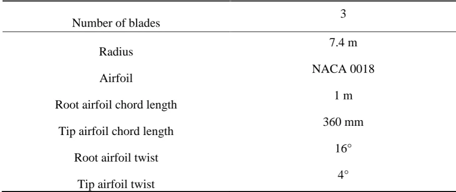
17 Table 1 - SB Parameters
647
Number of blades 3
Radius 7.4 m
Airfoil NACA 0018
Root airfoil chord length 1 m
Tip airfoil chord length 360 mm
Root airfoil twist 16°
Tip airfoil twist 4°
18 Figure 3 - 3D Plot of the CB Reproduced by MATLAB Program
650
19 Table 2 - Default Values for Defining the Curved Blade Shape
653 654
X- Offset Y – Offset Chord length, c (mm)
0 0 1645
0.2285 0.6 1337
0.4998 1.2 1091
0.8145 1.8 924
1.197 2.4 808
1.678 3 663
2.2164 3.6 509
2.7833 4.2 353
3.489 4.8 0
20 Figure 4 - The Skeleton (Centre Line) of the CB Fitted with Third Order Polynomial Function 658
21 Figure 5 - Chord Length Variation of the SB to Achieve CB
664
22 Figure 6 - Blade Spinal Axis Variation
668
23 Figure 7 - Inlet, Outlet, and Height Extension from the Turbine Blades
671
24 Table 3 Mesh size, CFD simulation time, and estimated CP for SST model at λ = 5.
676
Mesh Resolution
Coarse Mesh (M1)
Medium mesh
(M2) Fine mesh (M3)
Number of
nodes 79859 151740 230439
CFD
simulation time 4hrs 10mins 6hrs 16mins 9hrs 53mins
Estimated CP 0.3816 0.4169 0.4218
25 699
Table 4 Mesh size, CFD simulation time, and estimated CP for k-ε model at λ = 5.
700
Mesh Resolution
Coarse mesh (M4)
Medium mesh
(M5) Fine mesh (M6)
Number of
nodes 44064 92767 139506
CFD
simulation time 1hr 36mins 4hrs 41mins 5hrs 38mins
Estimated CP 0.2271 0.2586 0.2693
26 Figure 8 The power coefficients of all the investigated meshes in mesh independency study 738
27 787
788 789
Figure 9 Torque coefficient versus Tip speed ratio for k-ε and SST model medium meshes
790 791
792
28 823
824
Figure 10 Power coefficient versus tip speed ratio for k-ε and SST model medium meshes 825
29 873
874
Figure 11 - a) Meshed SB with Blades and Hub, b) SB Meshed Tip, c) Meshed 75% CB with 875
Blades and Hub, d) 75% CB Meshed Tip 876
877 878
a b
30 Table 5 - Mesh Parameters for all the Designed Blades (SST)
879
Blade Model
Mesh growth rate
Maximum mesh size
(mm)
Minimum mesh size
(mm)
Curvature normal angle
(°)
Number of nodes
SB 1.2 2500 75 15 151740
CB 25% 1.15 2100 50 13 195647
CB 50% 1.10 1800 45 11 226846
CB 75% 1.05 1500 40 10 252839
CB
100% 1.0 1150 35 10 309461
31 Figure 12 - Blade Pressure Distributions (Pressure Side) on a) SB, b) CB 25 %, c) CB 50%, d) CB 883
75%, and e) CB 100% 884
32 Figure 13 - SST Mid-height Lift Coefficient Distribution for Five Blade Designs
888 889
33 Table 6 - Mesh Parameters for the Designed Blades (LES-Smagorinsky)
893
Blade Model Mesh growth rate
Maximum mesh size
(mm)
Minimum mesh size
(mm)
Curvature normal angle
(°)
Number of nodes
SB 1.0 1150 65 10 427552
CB 25% 0.85 950 45 9 514842
CB 50% 0.7 820 40 7 690137
CB 75% 0.55 760 38 6 851326
CB 100% 0.4 680 35 6 912470
34 Figure 14 - CB 75% LES-Smagorinsky Convergence Monitoring with Respect to the Defined 896
Convergence Criteria. 897
35 Figure 15 - Lift Coefficient History Convergence Monitoring for the CB 75% Transient Solution. 901
36 Figure 16 – LES-Smagorinsky Blade Pressure Distributions (Pressure Side) on a) SB, b) CB 25 %, 907
c) CB 50%, d) CB 75%, and e) CB 100% 908
37 Figure 17 - LES – Smagorinsky Mid-height Lift Coefficient Distribution for Five Blade Designs 912
38 Figure 18 - Lift Coefficient Versus Angle of Attack for SST and LES CFD Simulations, at Inlet 916
Velocity 2.5m/s 917
918
39 Figure 19 - Power Coefficient Versus Output Power for the Designed Five Blades
921