https://doi.org/10.5194/ms-9-71-2018
© Author(s) 2018. This work is distributed under the Creative Commons Attribution 4.0 License.
Determining the range of allowable axial force
for the third-order Beam Constraint Model
Fulei Ma1, Guimin Chen1, and Guangbo Hao2
1School of Electro-Mechanical Engineering, Xidian University, Xi’an, Shaanxi 710071, China 2School of Engineering-Electrical and Electronic Engineering, University College Cork, Ireland
Correspondence:Guimin Chen ([email protected])
Received: 20 July 2017 – Revised: 22 January 2018 – Accepted: 2 February 2018 – Published: 16 February 2018
Abstract. The Beam Constraint Model (BCM) was developed for the purpose of accurately and analytically modeling nonlinear behaviors of a planar beam flexure over an intermediate range of transverse deflections (10 % of the beam length). The BCM is expressed in the form of Taylor’s expansion associated with the axial force. It has been found that the BCM may yield large predicting errors (>5 %) when the applied axial force goes beyond a certain boundary, even the deflection is still in the intermediate range. However, this boundary has not been clearly identified so far. In this work, we mathematically determine the non-dimensional boundary of the axial force by the condition that the strain energy expression of the BCM is a positive definite quadratic form, and by the buckling condition relate to compressing axial force. Several examples are analyzed to demonstrate the effects of the axial force on the modeling errors of the BCM. When using the BCM for modeling, it is always suggested to check if the axial force is within this boundary to avoid large modeling errors. If the axial force is beyond the boundary, the Chained Beam Constraint Model (CBCM) can be used instead.
1 Introduction
The Beam Constraint Model (BCM), developed by Awtar et al. (2007) a decade ago, offers a parametric and closed-form model for accurately and analytically capturing nonlinear be-haviors of a planar beam flexure over an intermediate range of transverse deflections (typically when transverse motion is less than 10 % of the beam length). The BCM is represented in the form of Taylor’s expansion associated with the axial force. The commonly-used BCM keeps the first-order terms of the axial force (Awtar et al., 2007), termed as the first-order BCM. The study objective of using the BCM is the slender beam (Euler beam) where beam length is 10 times longer than beam thickness in the bending direction. Due to its simplicity and analytical form, the BCM has been success-fully used in characterizing the performances of tilted-beam compliant mechanisms (Awtar et al., 2007; Awtar and Sen, 2010a),XY flexure mechanisms (Awtar and Slocum, 2007), cross-spring flexural pivots (Zhao et al., 2011), fully compli-ant bistable mechanisms (Chen and Ma, 2015; Masters and Howell, 2003; Wilcox and Howell, 2005), and compound multibeam parallelogram mechanisms (Hao, 2015; Hao and
Li, 2015). The BCM can also capture the first fixed-free beam buckling mode where the buckling loadpcrit= −2.5, which
is less than 1.3 % deviation from the classical beam buckling prediction ofpcrit= −π2/4.
It was demonstrated that the maximum error of the first-order BCM is less than 5 % for the non-dimensional transverse displacements (i.e., rotation θ and translation y=1Y /L, as illustrated in Fig. 1) within ±0.1, in-termediate deflection range, and the normalized axial force (p=P L2/(EI)) within ±10 (Awtar et al., 2007). The non-dimensional transverse displacements are confined within ±0.1 because BCM was derived based on the lin-earized beam-curvature assumptions (Awtar et al., 2007). Moreover, the range of the normalized axial force p was “empirically” restricted to [−10,10] to maintain less than 2 % truncation error (Awtar et al., 2010), which may limit the application of the BCM.
to check if the maximum axial forces carried by the flex-ible elements are within the BCM’s capability before us-ing it for modelus-ing. Moeen researched the nonlinear static load-displacement relationships of beam-based flexure mod-ules with an intermediate semi-rigid element (Moeen and Moeenfard, 2017) and considered the load-stiffening effects caused by axial loads using the BCM (Moeen and Moeen-fard, 2018). Hao (2015) showed that the results of the first-order BCM for compound multi-beam parallelogram mech-anisms significantly deviate from the results of the BCM in-cluding third-order terms of the axial force (termed as the third-order BCM) when the axial force exceeds a certain value. Although the third-order BCM is more accurate than the first-order BCM and extends the use of the BCM, what is the allowable axial force range of the third-order BCM re-mains unknown.
The determination of the range of allowable axial force includes finding the lower axial force boundary pl (i.e. the
maximum compressive axial force) and the upper bound-arypu(i.e. the maximum tensile axial force). Therefore, in
this paper, by using the conditions: (1) the positive definite quadratic condition of the strain energy expression of the BCM; (2) the characteristic that the BCM can only capture the first buckling mode (the deflected beam carrying no more than one inflection point), we mathematically derive the up-per and lower bounds of the allowable axial force for the third-order BCM, corresponding to the maximum tensile and compressive forces that the BCM can take, respectively. The third-order model is considered in this work because Hao (2015) showed that the BCM with the third-order terms ac-curately captures the relevant nonlinearities.
The rest of this paper is organized as follows. Section 2 briefly reviews the BCM equations and other related wor. The range of allowable axial force for BCM is mathematically obtained in Sects. 3.1 and 4.1. Three examples are utilised in Sects. 3.2 and 4.2 to demonstrate how the axial force influ-ences the modeling errors of the third BCM. Finally, Sect. 5 draws remarks of this study.
2 Literature review
2.1 Revisiting the Beam Constraint Model (BCM) Figure 1 illustrates a uniform cross-section beam flexure im-posed by a transverse forceF, an axial forceP and a moment M at its free end, resulting in transverse and axial deflec-tions1X,1Y and a tip slopeθ. The parameters of the beam include: the length L, the in-plane thicknessT, the out-of-plane thicknessH, and the Young’s modulus of the material E.A=H T andI =H T3/12 are the area and the second moment of inertia of the beam’s cross-section, respectively. The BCM formulates the nonlinear load-deflection relations of the beam using a set of parametric and closed-form equa-tions (Awtar et al., 2010). Following are the BCM equaequa-tions with the third-order terms of the axial force included (Wilcox
Figure 1.A simple beam flexure subject to combined force and moment loads.
and Howell, 2005; Hao et al., 2011):
f m
7= k
(0)
11 k
(0) 12
k12(0) k(0)22
!
y θ
+p k
(1)
11 k
(1) 12
k12(1) k(1)22
!
y θ
+p2 k
(2)
11 k
(2) 12
k12(2) k(2)22
!
y θ
+p3 k
(3)
11 k
(3) 12
k(3)12 k22(3)
! y θ (1)
x= t
2p
12L2−
1 2(y θ)
k11(1) k12(1) k12(1) k22(1)
!
y θ
−p(y θ) k
(2)
11 k
(2) 12
k12(2) k22(2)
! y θ −3 2p
2(y θ) k (3)
11 k
(3) 12
k12(3) k(3)22
!
y θ
−p3(y θ) g
(3)
11 g
(3) 12
g12(3) g(3)22
! y θ (2)
where the non-dimensional coefficientsk’s andg’s in the ma-trices are entirely independent of the beam shape and are re-ferred to as the beam characteristic coefficients, as listed in Table 1.tis the normalized thickness given ast=T /L. The variables,m,f andp, are the normalized load parameters andy andx are the non-dimensionalized (normalized) de-flection parameters, which are, respectively, given as:
m=ML EI , f =
F L2 EI , p=
P L2 EI , y=
1Y L , x=
1X L (3)
In addition, the third-order strain energy stored in the de-flected beam is formulated as (Awtar et al., 2010; Awtar and Sen, 2010b)
v=1 2
t2p2 12L2+
1 2(y θ)
k11(0) k12(0) k12(0) k22(0)
! y θ −1 2p
2(y θ) k11(2) k (2) 12
k12(2) k22(2)
!
y θ
−p3(y θ) k
(3)
11 k
(3) 12
k(3)12 k22(3)
!
y θ
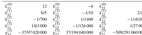
Table 1.Beam characteristic coefficients of the BCM matrices (Awtar et al., 2010).
k11(0) 12 k12(0) −6 k(0)22 4
k11(1) 6/5 k12(1) −1/10 k(1)22 2/15
k11(2) −1/700 k12(2) 1/1400 k(2)22 −11/6300
k11(3) 1/63 000 k12(3) −1/126 000 k(3)22 1/27 000
g(3)11 −37/97 020 000 g12(3) 37/194 040 000 g(3)22 −509/291 060 000
in whichvis the normalized strain energy with respect to the beam parameters given as
v=V L EI
whereV is the actual strain energy.
Note that the values of coefficients in Eqs. (1)–(4) are listed in Table 1.
2.2 Other related work
Hao et al. (2011) proposed an analytical method for modeling spatial deflection of a slender beam in its intermediate deflec-tion range, which combines two orthogonal beam constraint models (BCMs) with a torsional deflection model in the de-formed configuration. Based on the Timoshenko beam the-ory, the Timoshenko Beam Constraint Model (TBCM) was developed for the purpose of including shear effects in the model (Chen and Ma, 2015). Sen and Awtar (2013), Sen (2013) presented a spatial BCM (SBCM) for the purpose of accurately predicting the nonlinear spatial constraint charac-teristics of thin bisymmetric beams in their intermediate de-flection range (a bisymmetric beam refers to a beam whose cross section has equal moments of area and zero product of inertia). Ma and Chen (2016) proposed a Chained BCM (CBCM), which extends the BCM for modeling large planer deflections of beams in compliant mechanisms by utilizing a discretization strategy. The CBCM also alleviates the lim-itation of the maximum axial load of the BCM through dis-cretization. Chen and Bai (2015) further developed a Chained SBCM (CSBCM), which extends the SBCM for modeling large spatial deflections of bisymmetric flexible beams.
3 Upper bound of axial force
3.1 Determining upper bound
The strain energy stored in the deflected beam (Eq. 4) can be rewritten as:
v=V L EI =
1 2
t2p2 12L2+
1 2
y θ
Ke11(p) Ke12(p)
Ke21(p) Ke22(p)
y θ
(5)
where the first term on the right hand side of Eq. (5) repre-sents the strain energy due to stretching or compressing and
the following second term represents the strain energy due to bending. TheKe(p)’s in the strain energy formulation are
Ke11(p)=k11(0)−k11(2)p2−2k11(3)p3
Ke12(p)=k12(0)−k12(2)p2−2k12(3)p3
Ke21(p)=k12(0)−k12(2)p2−2k12(3)p3
Ke22(p)=k22(0)−k (2) 22p
2−2k(3) 22p
3 (6)
Because the strain energy expression of the third-order BCM is in a positive definite quadratic form for the case with a ten-sile axial force. The following conditions should be satisfied (Gilbert, 2009):
Ke11(p)>0
Ke11(p)Ke22(p)−Ke12(p)Ke21(p)>0 (7)
Combining Eqs. (6) and (7) and substituting the beam char-acteristic coefficients in Table 1 into the result yields the fol-lowing inequalities:
− p
3
31500+ p2
700+12>0 p6
476280000− 11p5 79380000+
p4 504000−
13p3 15750
+19p
2
1050+12>0 (8)
By solving the above inequalities, we have:
p <34.05 (9)
That is to say,pu=34.05 is the upper bound of axial force
when using the third-order BCM. It should also be noted that a Maximum truncation error of 2.4 % is occurred with the neglecting of the item with the fourth power ofpin the poly-nomial.
3.2 Case study
Figure 2.A fixed-guided beam in compliant parallelogram mecha-nism.
Table 2. Geometric parameters of the compliant parallelogram mechanism.H is the out-of-plane thickness of the beam.
Parameter H L T E
Value 20 mm 45 mm 1 mm 69 GPa
stage of the compliant parallelogram mechanism, the internal tensile axial force along the flexible beam can become very large while the transverse displacement1Y restrict to within 10 % of the beam length. The BCM is a reasonable choice to model the flexible beams in compliant parallelogram mech-anisms. Hao (2015) used the third-order BCM for modeling compound compliant parallelogram mechanisms. But when the transverse displacement1Y increases to a certain value, the difference between FEA and the BCM becomes large so that the third-order BCM may fail to predict the correct force-displacement relationship. The reason is that when the non-dimensional axial force p exceeds the upper boundary ax-ial forcepugiven in Eq. (9), the third-order BCM begins to
predict the inaccurate results, in other words, the third-order BCM should be used within the allowable upper boundary of the axial force. More details are followed below.
Since the compliant parallelogram mechanism has a sym-metric configuration, only a single beam of the mechanism is modeled. As shown in Fig. 3, the beam parameters listed in Table 2 are identical to those used in Hao (2015). The co-ordinateXOY is established with its origin at the fixed end attached to the base. The normalized end displacement can be written as:
x=0, y=1Y
L , θ=0 (10)
Let 1Y increase from the initial position to 0.1Land sub-stitute Eq. (10) into Eqs. (1) and (2), the relationships of the reaction forceFy and the normalized internal axial forcep along the beam against the transverse displacement1Y can be illustrated in Figs. 4 and 5, respectively.
A finite element model of the compliant parallelogram mechanism was built with the ANSYS software where the beam was meshed into 200 elements with Beam 188. The
Figure 3.A beam flexure in compliant parallelogram mechanism.
0 0.5 1 1.5 2 2.5 3 3.5 4 4.5
x 10−3 0
500 1000 1500 2000 2500 3000 3500 4000
ΔY (m)
FY
(N)
Third−order BCM CBCM FEA
Figure 4.Comparion of the load-displacement relationship of the compliant parallelogram mechanism.
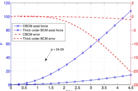
results are also plotted in Fig. 4. It can be seen from Fig. 4 that the results obtained by the third-order BCM clearly de-viate from FEA results afterp exceedspu. The maximum
error of the BCM comparing with FEA is 20 % when the non-dimensional end displacement is 0.1. The axial tensile loads are also given in Fig. 5 which shows that the maximum internal axial tensile force of the third-order BCM is larger than 100, which is much larger the upper boundary of the allowable forcepufor the BCM.
In order to show the effect of the axial tensile force on the modeling error of the third-order BCM, we compare its re-sults to those obtained using CBCM. Considering the effec-tiveness and efficiency, the CBCM results were obtained by dividing the beam into 3 elements (Ma and Chen, 2016). In such a way, the element axial tensile loads by normalization is reduced tope=P(L/3)2/EI=p/9 which is ensured to
be less thanpu. The maximum error of the CBCM is reduced
Figure 5.Comparision of normalised axial force and error of the compliant parallelogram mechanism.
noted that the maximum stress in the beams may exceed the yield stress of the material when the mechanism translates 0.1Lalong the transverse direction, inducing failure of the mechanism.
4 Lower bound of axial force
4.1 Determining lower bound
When the compressive force applied at the end of a flexible beam exceeds a certain value p, the beam can buckle due to the instability of the beam. Actually, the buckling corre-sponds to a singularity of the stiffness matrix in the force-displacement formula. This buckling load is also defined as the critical loadfcr. As the third-order BCM is derived based
on a fixed-free beam shown in Fig. 1, the compressive force related to the buckling can be calculated by setting the deter-minant of the nonlinear bending stiffness matrix to be zero. Rewrite Eq. (1) as:
f m
=Ks
y θ
=
Ks11(p) Ks12(p)
Ks21(p) Ks22(p)
y θ
(11)
whereKsis the nonlinear stiffness matrix that relates the tip
loads and the tip displacements, in which each
Ks11(p)=k11(0)+k11(1)p+k11(2)p2+k11(3)p3
Ks12(p)=k12(0)+k12(1)p+k12(2)p2+k12(3)p3
Ks21(p)=k12(0)+k12(1)p+k12(2)p2+k12(3)p3
Ks22(p)=k22(0)+k (1) 22p+k
(2) 22p
2+k(3) 22p
3 (12)
By letting the determinant of Ks be zero and using the
pa-rameters given in Table 1, the following equation can be
ob-tained:
p6 1 905 120 000−
11p5 158 760 000+
71p4 1 512 000−
109p3 63 000
+277p
2
2100 + 26p
5 +12=0 (13)
Equation (13) is solved to obtain the following roots:
p=
47.16+83.74i 47.16+83.74i 31.82+61.26i 31.82−61.26i −23.50 −2.47
(14)
The first four roots are complex numbers with no physical meaning, which thus are neglected. The fifth and sixth roots are real solutions associated with two buckling modes. How-ever, when the normalized compressive axial force increases to the lower one,p= −2.47, the stiffness matrixKswill
ex-hibit a singularity, which the beam buckles, so the larger one (fifth root) is not considered. The axial forcefa
correspond-ing to the first bucklcorrespond-ing mode of fixed-free beam is given as:
pa=p= −2.47 (15)
It is indicated in the knowledge of mechanics of materials (Timoshenko, 2001) that the critical load fcr
correspond-ing to bucklcorrespond-ing is closely related to the boundary condi-tion applying at the end of the flexible beam. In order to find the lower boundary of the axial force that defines the third-order BCM formula, we consider others boundary con-ditions: fixed-pivoted and fixed-fixed, as illustrated in Fig. 6. The critical loads corresponding to the free, fixed-pivoted and fixed-fixed beam buckling modes (Fig. 6) can be written, respectively, as:
pa=fcr
pb=
400 49fcr
pc=16fcr (16)
As the BCM can only capture the first buckling mode, ac-cording to the results in Eq. (16), the lower boundary of the axial force,pl, for different boundary conditions can be
ex-pressed as:
pl=
−2.47 Fixed-free beam
−20.16 Fixed-pivoted beam −39.52 Fixed-fixed beam
(17)
4.2 Case study
Figure 6.(a)fixed-free beam buckling;(b)fixed-pivot beam buck-ling;(c)fixed-fixed beam buckling.
The negative stiffness and the bistable behaviors have always complicated the modeling. Furthermore, the compressive ax-ial force along the flexible beam can become very large while the transverse displacement1Y (perpendicular to the beam) is still limited within 10 % of the beam length. Among all the methods, the BCM is a prior choice to model the behaviors of bistable mechanisms. But, when the compressive axial force exceeds a certain value, the BCM results may show an error. In this section, two different bistable mechanism examples were used to demonstrate the effectiveness of the range of the axial force allowable for the BCM. The first example is chosen to show the performance of the BCM when the com-pressive axial force is larger than the allowable lower bound-ary. The second example, on the contrary, is a case for the compressive axial force within the allowable lower bound-ary.
It should be demonstrated that for both examples the non-dimensional transverse displacements perpendicular to the beam are strictly limited within ±0.1 in all the deflected cases in order to guarantee the effectiveness of the linearized approximate expression for curvature. Details are elaborated as follows.
Considering that the geometry and loading of the bistable mechanism are symmetrical, a single fixed-guided limb is chosen to analyze. Figure 8 illustrates the schematic of the fixed-guided beam. Establish the coordinate system along the beam with its origin placed at the fixed end and denote the initial angle of the fixed-guided beam asβ. The end displace-ment can be written as:
x=1Ycosβ L , y=
1Ysinβ
L , θ=0 (18)
Wherex is the normalized displacement along the beam,y is the normalized displacement perpendicular to the beam, andθis the tip rotation of the beam, which stays unchanged during the deflection. The parameters of Example I are given in Table 3. Let1Y increase from the initial position to 0.1L with the help of submitting Eq. (18) into Eqs. (1) and (2),
As-fabricated position
Deflected position
T
Shuttle
L
β
Figure 7.A bistable mechanism.
Figure 8.Schematic of the bistable mechanism.
the relationships of the reaction forceFyand the normalized internal axial force along the beam against the transverse dis-placement1Y can be obtained as shown in Figs. 9 and 10, respectively.
Modelling the deflected beam of Example I using an FEA model built with the ANSYS software (the beam was meshed into 200 elements with Beam 188), the FEA force-displacement relationship is also plotted in Fig. 9. It can be observed that the results achieved by the BCM are consis-tent well with those obtained by FEA at the beginning of the force-deflection curve. When the tip displacement 1Y getting larger, the third-order BCM fails to predict the force-displacement relationship. The error between the results ob-tained by the BCM and FEA is up to 60 %, as shown in Fig. 10. The normalized internal axial force along the beam during the deflection is also illustrated in Fig. 10 (using the othery axis for comparison in the figure). It can be shown that when the normalized compressing axial force magnitude pis larger than 39.52, which exceeds the lower boundary of the axial forcepl, the third-order BCM fails to deal with this
problem.
Table 3.Parameters of the examples.H is the out-of-plane thick-ness of the beam.
Parameter Example I Example II
H 10 mm 10 mm
L 80 mm 60 mm
θ 3.5◦ 2◦
t 1 mm 1 mm
E 1.379 GPa 1.379 GPa
0 1 2 3 4 5 6 7 8
x 10−3
−0.3 −0.2 −0.1 0 0.1 0.2 0.3 0.4 0.5
ΔY (m)
Fy (N)
Third−order BCM FEA
CBCM
Figure 9.Comparison of the load-displacement relationship of Ex-ample I.
curve obtained by the CBCM is given in Fig. 9. The error of the force displacement relationship obtained by comparing the CBCM and FEA results is also plotted in Fig. 10 and the maximum error is less than 1 %.
As for Example II, we also model it using both the third-order BCM and FEA methods. The force-displacement re-lationship can be obtained as shown in Fig. 11. It can be seen that the results obtained by the BCM and FEA match well and the maximum error is 2.5 % as shown in Fig. 12. The normalized internal axial loads along the beam during the deflection are also displayed in Fig. 12 for comparison. The maximum compressing axial force magnitudep=21 is lower than|pl|and the tip displacement 1Y is kept in the
intermediate deflection range, so the third-order BCM can correctly capture the force-displacement of the mechanism.
5 Conclusions
In this work, we determine the range of the allowable axial force of the third-order BCM. The upper boundpuare equal
to 34.05, and the lower boundpl is set to different values
with respect to different boundary conditions:pl= −2.47 for
fixed-free buckling,pl= −20.16 for fixed-pivoted buckling,
andpl= −39.52 for fixed-fixed buckling. Generally
speak-ing, a complaint mechanism is analyzed in a series of in-cremental displacement steps or a series of inin-cremental load
0 1 2 3 4 5 6 7 8
x 10−3
−100 −75 −50 −25 0
ΔY (m)
p
0 1 2 3 4 5 6 7 8
x 10−3 −100 −50 0 50 100
Error (%)
Third−order BCM axial force CBCM axial force CBCM error Third−order BCM error p = −39.52
Figure 10.Comparision of normalized axial force and error of Ex-ample I.
0 0.5 1 1.5 2 2.5 3 3.5 4
x 10−3 0
0.05 0.1 0.15 0.2 0.25 0.3 0.35 0.4 0.45
ΔY (m)
Fy
(N)
Third−order BCM FEA
Figure 11.Comparion of the load-displacement relationship of Ex-ample II between FEA and the BCM.
steps. At each step, the proposed bounds should be used to check the axial forcepto guarantee the effectiveness of the BCM equations.
Three examples are analyzed to demonstrate the effects of the axial force on the modeling errors of the third-order BCM, and the CBCM with 3 elements were used in this work to guarantee the accuracy of the results so that they can be used as the exact solutions for the purpose of compar-ison. Firstly, the case that the axial tensile force is beyond the upper boundary of the allowable force is given showing the effectiveness ofpu. Secondly, the cases that the axial
com-pressing forces arewithin and beyond the lower boundary of the allowable force are presented, the results have verified the effectiveness of the value ofpl. When using the third-order
[í
í í í
Δ<P
S
[í
í í í í í
(UURU
Normalized axial force Error
Figure 12.Comparision of normalized axial force and error of Ex-ample II.
For the non-dimensional transverse displacements within ±0.1 and the normalized axial force (p=P L2/(EI)) within [pl, pu], the majority of the modeling errors of the third-order
BCM comes from the truncation of the Taylor’s expansion. It should be acknowledged that the CBCM expands the range of the allowable axial force for the BCM through discretizing the beam (Ma and Chen, 2016). For exam-ple, if a beam is discretized into two elements with equal length (the length of each element is L/2), then the corre-sponding normalized compressive axial force of the model for each element becomes 1/4 times of the original nor-malised one according to Eq. (3). For a beam that carries an axial force beyond the derived bounds in this paper, the chained Beam- Constraint-Model (CBCM) (Ma and Chen, 2016, 2014) and the comprehensive elliptic integral solution (Zhang and Chen, 2013) can be used to model it instead de-spite they much less analytical than the third-order BCM.
Data availability. All the data used in this manuscript can be ob-tained on request from the corresponding author.
Competing interests. The authors declare that they have no con-flict of interest.
Acknowledgements. The authors gratefully acknowledge
the financial support from the National Natural Science Foun-dation of China under Grant No. 51675396, and the Fun-damental Research Funds for the Central Universities under No. JB170403/K5051204021.
Edited by: Xianwen Kong
Reviewed by: two anonymous referees
References
Awtar, S. and Sen, S.: A Generalized Constraint Model for Two-Dimensional Beam Flexures: Nonlinear Load-Displacement Formulation, ASME J. Mechan. Des., 132, 081008, https://doi.org/10.1115/1.4002005, 2010a.
Awtar, S. and Sen, S.: A Generalized Constraint Model for Two-Dimensional Beam Flexures: Nonlinear Strain En-ergy Formulation, ASME J. Mechan. Des., 132, 081009, https://doi.org/10.1115/1.4002006, 2010b.
Awtar, S. and Slocum, A.: Constraint-Based Design of Parallel Kinematic XY Flexure Mechanisms, ASME J. Mech. Des., 129, 816–830, 2007.
Awtar, S., Slocum, A., and Sevincer, E.: Characteristics of Beam-Based Flexure Modules, ASME J. Mechan. Des., 129, 625–639, 2007.
Awtar, S., Shimotsu, K., and Sen, S.: Elastic Averaging in Flexure Mechanisms – A Three-Beam Parallelogram Flex-ure Case Study, ASME J. Mech. Robot., 2, 041006, https://doi.org/10.1115/1.4002204, 2010.
Chen, G. and Bai, R.: Modeling Spatial Deflections of Flex-ible Beams in Compliant Mechanisms using a Chained Spatial-Beam-Constraint-Model (CSBCM), Proceedings of the ASME Design Engineering Technical Conferences & Comput-ers and Information in Engineering Conference, Boston, USA, DETC2015-46387, 2–5 August 2015.
Chen, G. and Ma, F.: Kinetostatic modeling of fully com-pliant bistable mechanisms using Timoshenko beam constraint model, ASME J. Mech. Des., 137, 022301, https://doi.org/10.1115/1.4029024, 2015.
Chen, G., Wilcox, D., and Howell, L.: Fully compliant dou-ble tensural tristadou-ble micromechanisms (DTTM), J. Mi-cromech. Microeng., 19, 025011, https://doi.org/10.1088/0960-1317/19/2/025011, 2009.
Gilbert S.: Introduction to Linear Algebra (Fourth Edition), Welles-ley Cambridge Press, MA, 2009.
Hao, G.: Extended Nonlinear Analytical Models of Compliant Parallelogram Mechanisms: Third-order Models, T. Can. Soc. Mech. Eng., 39, 71–83, 2015.
Hao, G. and Li, H.: Nonlinear Analytical Modeling and Char-acteristic Analysis of a Class of Compound Multibeam Par-allelogram Mechanisms, ASME J. Mech. Robot., 7, 041016, https://doi.org/10.1115/1.4029556, 2015.
Hao, G., Kong, X., and Reuben, R.: A nonlinear analysis of spatial compliant parallel modules: multi-beam modules, Mech. Mach. Theory, 46, 680–706, 2011.
Holst, G., Teichert, G., and Jensen, B.: Modeling and experi-ments of buckling modes and deflection of fixed-guided beams in compliant mechanisms, ASME J. Mech. Des., 133, 051002, https://doi.org/10.1115/1.4003922, 2011.
Howell, L. L.: Compliant Mechanisms, Wiley, New York, 2001. Ma, F. and Chen, G.: Modeling of V-Shape Thermal In-Plane
Microactuator Using Chained Beam-Constraint-Model, Interna-tional Conference on Manipulation, Manufacturing and Mea-surement on the Nanoscale (3M-NANO 2014), Taipei, p. 296– 300, 27–31 October 2014.
Beam-Constraint-Model (CBCM), ASME J. Mech. Robot., 8, 021018, https://doi.org/10.1115/1.4031028, 2016.
Masters, N. and Howell, L.: A self-retracting fully compliant bistable micromechanism, J. Microelectromech. Syst., 12, 273– 280, 2003.
Moeen, R. and Moeenfard, H.: A Constraint Model for Beam Flex-ure Modules with an Intermediate Semi-Rigid Element, Int. J. Mech. Sci., 122, 167–183, 2017.
Moeen, R. and Moeenfard, H.: Load-displacement behavior of fun-damental flexure modules interconnected with compliant ele-ments, Mech. Mach. Theory, 120, 120–139, 2018.
Sen, S.: Beam constraint model: generalized nonlinear closed-form modeling of beam flexures for flexure mechanism design, PhD Dissertation, the University of Michigan, 2013.
Sen, S. and Awtar, S.: A closed-form nonlinear model for the constraint characteristics of symmetric spatial beams, ASME J. Mech. Des., 135, 031003, https://doi.org/10.1115/1.4023157, 2013.
Timoshenko, S.: Strength of Materials: Part I, Elementary Theory and Problems, 2nd ed., Lancaster Press, PA, 2001.
Wilcox, D. and Howell, L.: Fully compliant tensural bistable mi-cromechanisms (FTBM), J. Microelectromech. Syst., 14, 1223– 1235, 2005.
Zhang, A. and Chen, G.: A Comprehensive Elliptic Integral So-lution to the Large Deflection Problems of Thin Beams in Compliant Mechanisms, ASME J. Mech. Robot., 5, 021006, https://doi.org/10.1115/1.4023558, 2013.