R E S E A R C H
Open Access
Handling missing weak classifiers in boosted
cascade: application to multiview and
occluded face detection
Pierre Bouges
1*, Thierry Chateau
1*, Christophe Blanc
1and Gaëlle Loosli
2Abstract
We propose a generic framework to handle missing weak classifiers at testing stage in a boosted cascade. The main contribution is a probabilistic formulation of the cascade structure that considers the uncertainty introduced by missing weak classifiers. This new formulation involves two problems: (1) the approximation of posterior probabilities on each level and (2) the computation of thresholds on these probabilities to make a decision. Both problems are studied, and several solutions are proposed and evaluated. The method is then applied to two popular computer vision applications: detecting occluded faces and detecting faces in a pose different than the one learned. Experimental results are provided using conventional databases to evaluate the proposed strategies related to basic ones.
Keywords: Pattern recognition; Supervised learning; Object detection; Missing data; Adaptation; Face
1 Introduction
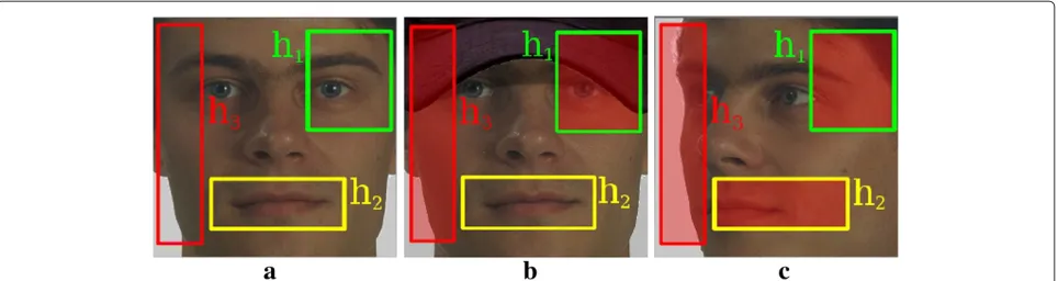
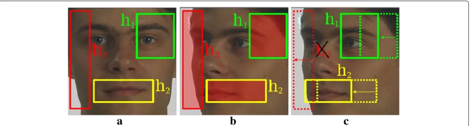
Boosted cascade is a popular technique in the field of object detection. Boosting algorithms are learning algo-rithms that combine weak classifiers to produce a strong classifier. A weak classifier is a classifier that is slightly better than random to detect objects. A strong classifier is a classifier which is supposed to have high detection performance. When a candidate area is to be processed, each weak classifier is applied to a part of this area (see Figure 1a). In many computer vision detection applica-tions, the algorithm has to handle partial observaapplica-tions, i.e., the object is partially occluded (see Figure 1b) or has to be detected in a pose different than the one learned (see Figure 1c). In such situations, weak classifiers that are in charge of classifying occluded areas tend to corrupt the final decision, i.e., the candidate area will often be classi-fied as a non-object. Existing solutions consist in defining a set of finite occlusion configurations (or a set of pose configurations) and train multiple boosted cascades, one per configuration (see [1] for an example of multiview face detection). In the proposed solution, multiple training is
*Correspondence: [email protected]; [email protected]
1Institut Pascal, Université Blaise Pascal 24, avenue des Landais, Aubière cedex 63177, France
Full list of author information is available at the end of the article
avoided (only one classifier is used) and occluded weak classifiers are considered as missing data. A weak classifier is occluded when the data window of the weak classifier has hit an occluded part of the face.
Missing data in classification can be divided into two subproblems: (1) missing data at training stage and (2) missing data attestingstage. In this paper, we assume that missing data only occur at testing stage and that training is done with complete data. A recent study on missing data at testing stage can be found in [2] where Saar-Tsechansky and Provost evaluate different methods to handle missing data at testing stage. They compare two kinds of approach: reduced models and predictive value imputation. Their study does not focus on boosted cascades; the solution we propose in this paper is, to our knowledge, the first algorithm that handles missing data in a boosted cascade without modifying the initial training. Most existing solu-tions are based on learning algorithms that are designed to be robust to missing data. For example, Smeraldi et al. [3] used a modified version of adaptive boosting (AdaBoost) where weak classifiers can abstain when a feature is miss-ing. Another algorithm was proposed by Globerson and Roweis [4] which is built to be robust to feature dele-tion. In the same way, Dekel and Shamir [5] improved this idea with an algorithm robust to feature deletion and fea-ture corruption. Chen et al. proposed [6] a solution to
Figure 1Subwindows of weak classifier on an upright face, an occluded face, and a turned face.(a)An example of learned weak classifiers. Each one is in charge of classifying a subwindow. In(b), the face is occluded, and the subwindow ofh1andh3, filled in red, might be classified as non-face. Similarly, the face in(c)is turned 45°, and all subwindows might be classified as non-face.
detect occluded faces using only one upright face classi-fier, but they lost the cascade structure resulting in a high detection time.
Here we propose a generic solution to the problem of occluded object detection where occluded weak classifiers are considered as unavailable. Unavailable weak classifiers are seen as missing data, and this fact is incorporated in the cascade structure. We evaluate the proposed method for two different applications: (1) detecting occluded faces and (2) detecting faces in a pose different than the one learned. For each application, we explain how weak clas-sifiers can be considered as available or not. Our method differs from former studies [1,7] in two aspects: the pro-posed solution does not need the training of multiple classifiers, and, as opposed to existing methods where classifiers are designed to detect objects in a specific pose or with specific occlusions, the proposed solution relies on only one classifier that can adapt to specific poses or occlusions.
Section 2 presents the principle of boosted cascade. A new algorithm that handles missing weak classifiers in a boosted cascade is then detailed in Section 3. Application to occluded faces is presented in Section 4, followed by application to multiview face detection in Section 5. The proposed method is then evaluated in Section 6.
2 Boosted cascade overview
This section presents the principle of boosted cascade. The boosting algorithm was introduced by Schapire [8], and many extensions have been proposed. The main idea is to combine the performance of many weak classifiers to produce a powerful strong classifier. The goal is then to perform binary classification. In this paper, we focus on realboosting algorithms (e.g., Real AdaBoost, LogitBoost, or Gentle AdaBoost) which means that weak classifiers are real-valued functions.
LetL= {(xi,yi)}Ni=1be a training set wherexiare train-ing examples and yi ∈ {−1, 1} are their corresponding
labels (1 is for the object class, also called positive class). Given this set, a real boosting algorithm iteratively findsT weak classifiershtto form a strong classifier sign(H(x))= sign(Tt=1ht(x)) where x is a sample to be classified. Moreover, sign(ht(x))gives the label ofxpredicted byht, and the value|ht(x)|represents the confidence of the pre-diction. Each training example xi is an image Ri of the object or non-object, and each weak classifierhtis learned on a set of subwindows{rti}Ni=1which correspond to dis-criminative areas in all images{Ri}Ni=1(see Figure 1a for an example of such subwindows).
To speed up classification, Viola and Jones [9] proposed a cascade structure where several strong classifiers are associated into successive levels. The idea is that the first strong classifiers reject most of the negative examples, while the last strong classifiers try to discriminate positive examples from hard negative examples. In such cascades, strong classifiers are slightly changed into sign(Hj(x) −
available. The following section presents a generic frame-work to use this cascade when some weak classifiershjt are missing at testing stage.
3 Handling missing weak classifiers
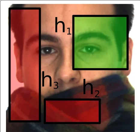
This section presents the problem of missing weak classi-fiers in a boosted cascade, and solutions to this problem are then detailed. To explain our motivation, suppose we want to detect a face occluded by a scarf. In such a sit-uation, all subwindows located on the lower part of the face will overlap the scarf, and thus all associated weak classifiers will tend to classify these subwindows as non-face. On the other hand, subwindows on the upper part of the face are likely to be classified as face. This is why we propose to consider weak classifiers corresponding to fea-tures on the lower part of the face as unavailable. Weak classifiers on the upper part of the face remain available. An example with three weak classifiers is given in Figure 2. In this section, it will be assumed that some weak clas-sifiers are available and some are unavailable. We do not focus on why a weak classifier is available or not. These details will be given in Sections 4 and 5 which are ded-icated to occluded face detection and to multiview face detection.
3.1 Naive approach
Suppose that we want to classify a samplexwith a strong classifier sign(H−α)whereHis made up of a set of weak classifiers{h1,. . .,hT}. Suppose also that onlyp<Tweak
Figure 2Example of a situation where some weak classifiers are missing.The face is occluded by a scarf. Rather than using all weak classifiers, we propose to use only the weak classifiers that should classify the upper part of the face (in green in the figure). The others, in red, are considered as unavailable.
classifiers are available, given by {ha1,. . .,hap}. The set
of unavailable weak classifiers is defined as{hu1,. . .,huq} whereq=T−p. In such a situation, the easiest strategy to classifyxconsists in setting all unavailable weak classifiers to zero, i.e.,hu1(x)= · · · =huq(x)=0. If we noteHa(x)=
p
t=1hat(x), the strong classifier becomes sign(Ha−α). By applying this principle to all cascade levels, the set of strong classifiers becomes{sign(H1a−α1),. . ., sign(HKa− αK)}. To sum up, the naive approach consists in setting all unavailable weak classifiers to zero and keeping all cas-cade thresholds unchanged. This approach will be used as our baseline in the experiments section and will be referred to as ‘naive approach’.
3.2 Probabilistic formulation of a boosted cascade
In a real boosting algorithm, the predicted label y ∈ {−1, 1} of a sample xcan be seen as a discrete random variable andH(x)can be interpreted as the probability ofy being an object given the examplex(also called the poste-rior probability) using the following sigmoid function [10]:
P(y=1|x)=eH(x)/(eH(x)+e−H(x)). (1) Thus, each cascade level computesP(yj=1|x)whereyj is the predicted label of the levelj. If a samplexreaches the level j, it means that it has passed all previous lev-els and is a candidate for an object. This is why we have P(yj = 1|x) = P(yj = 1|x,y1 = 1,. . .,yj−1 = 1). When weak classifiers are missing, uncertainty is introduced on each predicted labelyj. This uncertainty is not considered in the probabilityP(yj = 1|x,y1 = 1,. . .,yj−1 = 1) as labelsy1,. . .,yj−1are supposed to be positive. This is why we propose to computeP(y1 = 1,. . .,yj = 1|x)on level
j. Thus, the predicted label on leveljwill also depend on predicted labels of level 1 toj−1. In the rest of the paper, the eventy1=1,. . .,yj=1 will be notedy1:j=1 to sim-plify the notation. To computeP(y1:j=1|x), the following rule is used:
P(A,B|C)=P(B|A,C)P(A|C). (2)
This rule gives:
P(y1:j=1|x)= P(yj=1|x,y1:j−1=1)
×P(y1:j−1=1|x) ∀j>1. (3)
By applying this rule recursively, we get:
P(y1:j=1|x)= j
i=2
P(yi=1|x,y1:i−1=1)
×P(y1=1|x) ∀j>1 (4)
=
j
i=1
P(yi=1|x). (5)
based on a probabilistic cascade formulation. In our case, we use a probabilistic formulation to handle the fact that some weak classifiers are missing at testing stage.
In a conventional cascade formulation, each level j applies a strong classifier Hj to x and compares Hj(x) with a threshold αj. With the probabilistic formulation, all thresholds αj disappear and new thresholds βj are introduced. Indeed, we haveP(yj=1|x)≤1, and so:
j
i=1
P(yi=1|x)≤ j−1
i=1
P(yi=1|x)
≤ · · · ≤P(y1=1|x) (6)
Equation 6 shows that ifP(y1:j = 1|x) is lower than a value βj, the cascade process should stop because
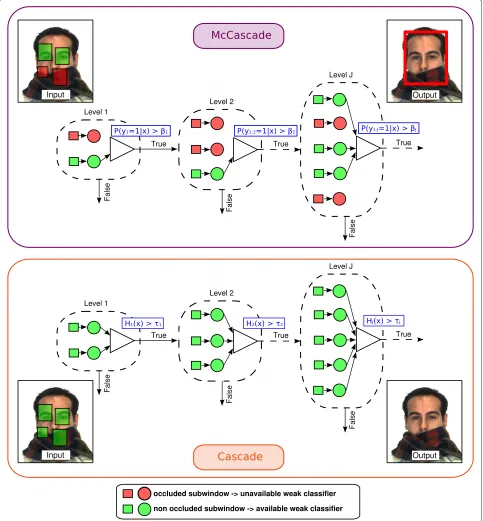
P(y1:j+1 = 1|x),. . .,P(y1:K = 1|x)will be even smaller. In the proposed framework, a strong classifier is defined as sign(P(y1:j = 1|x) − βj). The complete modified boosted cascade is then defined by the set of strong clas-sifiers {sign(P(y1 = 1|x)− β1), sign(P(y1:2 = 1|x) − β2),. . ., sign(P(y1:K = 1|x)−βK)}. In the following, we refer to this modified cascade as boosted McCascade for boosted cascade with missing classifiers. Figure 3 sums up the differences between a cascade structure and a McCas-cade structure. Section 3.4 explains how valuesβ1,. . .,βK are computed, and the following section focuses on the estimation ofP(yj=1|x).
3.3 Posterior probability estimation
When weak classifiers are missing, the probabilityP(y= 1|x) can no longer be computed and an approximation must be used. We propose three different approximation strategies to do this:
• The simplest strategy to estimateP(y=1|x)is to compute a probability based on available weak classifiers. Thus, we definePboost(y=1|x)as:
Pboost(y=1|x)=. eHa(x)/(eHa(x)+e−Ha(x)). (7)
• A second strategy, notedPknn(y=1|x), tries to
benefit from the initial training. Indeed, each training examplexiprovides a set of weak classifier values hxi=(h1(xi),. . .,hT(xi))and an associated labelyi. All these weak classifier values form a set
H= {(hxi,yi)}Ni=1, and the subset of available weak classifiers formHa= {(haxi,yi)}Ni=1where
haxi =(ha1(xi),. . .,hap(xi)). The resulting setHais used as a training set to approximateP(y=1|x)with the help of thek -nearest neighbor (k -nn) algorithm. Given a samplex, its associated available weak classifier scoreshax=(ha1(x),. . .,hap(x))are first computed. Then, thek -nn algorithm searches the k nearest neighbors of the pointhaxin the spaceHa. Considering the labels{y∗1,. . .,y∗k}of thek nearest
neighbors, the probabilityPknn(y=1|x)is computed
as:
Pknn(y=1|x)=. k
i=1 1l{y∗
i=1}
k , (8)
where1lpred=1if the predicate (pred) is true and
1lpred=0otherwise. Figure 4 illustrates the
computation ofPknn(y=1|x)when two weak
classifiers are available.
• An additional strategy, notedPcomb(y=1|x),
consists in combining the two previous methods as the simplest way:
Pcomb(y=1|x)=.
Pboost(y=1|x)+Pknn(y=1|x)
2 .
(9)
3.4 Boosted McCascade threshold estimation
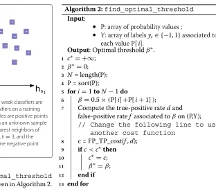
Before a McCascade can be used to classify a samplex, the thresholdβ1,. . .,βK must be estimated. The thresh-oldβ1,. . .,βKestimation can be seen as the training stage of a McCascade. This is achieved through an iterative pro-cedure which uses setsSpandBfrom the initial training stage. This procedure is described in Algorithm 1. At iter-ationj, the thresholdβjof the leveljis computed using the following scheme: all probabilitiespji=. P(y1:j=1|xi) are first computed. Then, the set of probabilities{pji}Ni=1 is sorted andβjis chosen among the set of finite values
˜
pji =. 0.5(pji + pj(i+1)),i ∈ {1,. . .,N − 1}. The
func-tionfind_optimal_threshold(see line 14) finds the
threshold that minimizes a cost function defined on false-positive and true-false-positive rates. Contrary to the initial cascade where each level ensures reaching a true-positive rate of at leastdminwith a false-positive rate less thanfmax, the McCascade cannot guarantee the same performance. The cost function’s goal is to ensure that each threshold found provides a performance close to the initial cascade performance. Three cost functions are proposed:
• FP_cost is defined on the false-positive ratefβ associated to a thresholdβ:
FP_cost(fβ)=. max(0,fβ−fmax). (10)
The false-positive ratefβis computed on the training examples. Using this function means that the threshold found provides a false-positive rate which is as close as possible tofmax(it remains greater or equal tofmax).
• TP_cost is defined on the true-positive ratedβ associated to a thresholdβ:
TP_cost(dβ)=. max(0,dmin−dβ). (11)
Figure 3Differences between a cascade and a McCascade for the classification of a samplex.In a cascade, all weak classifiers are used. At levelj,Hj(x)is computed and is compared to the thresholdτj. An occluded face is most of the time rejected because occluded subwindows corrupt
the decision on each level. In a McCascade, only a subset of weak classifiers is used. In the figure, only weak classifiers in charge of classifying the upper part of the face are used. At levelj,P(y1:j=1|x)is computed and is compared to the thresholdβj. An occluded face is most of the time
detected. In contrast to the decision at leveljof a cascade, the decision at leveljof a McCascade incorporates the decision of previous levels.
function will ensure a true-positive rate close todmin (it remains lower or equal todmin).
• FP_TP_cost is defined on both false-positive and true-positive rates:
FP_TP_cost(fβ,dβ)=. FP_cost(fβ)+TP_cost(dβ). (12)
This last cost function is a compromise between a false-positive rate offmaxand a true-positive rate of
Figure 4Computation ofPknn(y=1|x).Two weak classifiers are available:ha1andha2. Applying these weak classifiers on a training
database gives the set of pointsHa(the red circles are positive points and the blue squares are negative points). Given an unknown sample x,ha1(x)andha2(x)are computed and theknearest neighbors of (ha1(x),ha2(x))are searched inHa. In the figure,k=3, and the
nearest neighbors are two positive points and one negative point which leads toPknn(y=1|x)=2/3.
A detailed version of find_optimal_threshold
with the cost function FP_TP_cost is given in Algorithm 2. Once all the thresholds β1,. . .,βK are estimated, the McCascade can be used to classify any unknown samplex.
Algorithm 1:McCascade threshold estimation
Input:
• Positive image setSp; • Background image setB; • Set of probability law
{P(y1=1|x),. . .,P(y1:K =1|x)}; Output: Thresholdsβ1,. . .,βK.
1 forj=1toKdo 2 ifj=1then
3 Create the negative image setSnby randomly extracting areas in images ofB;
4 else
5 Apply the McCascade{sign(P(y1=
1|x)−β1),. . ., sign(P(y1:j−1=1|x)−βj−1)}on images ofBto generate false-positives which are used to create the negative image setSn;
6 end if
7 P= ∅; 8 Y= ∅;
9 foreachexample(xi,yi)∈Sp∪Sndo
10 Compute the probabilitypji=P(y1:j=1|xi); 11 P[i]=pji;
12 Y[i]=yi;
13 end foreach
14 βj=find_optimal_threshold(P, Y);
15 end for
Algorithm 2:find_optimal_threshold
Input:
• P: array of probability values ;
• Y: array of labelsyi∈ {−1, 1}associated to each value P[i].
Output: Optimal thresholdβ∗. 1 c∗= +∞;
2 β∗=0; 3 N= length(P); 4 P = sort(P);
5 fori=1toN−1do
6 β =0.5×(P[i]+P[i+1]);
7 Compute the true-positive ratedand false-positive ratef associated toβon (P,Y);
// Change the following line to use another cost function
8 c = FP_TP_cost(f,d); 9 ifc<c∗then 10 c∗=c; 11 β∗=β;
12 end if
13 end for
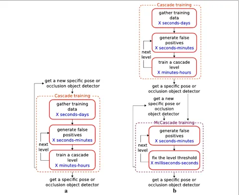
3.5 Cascade and McCascade training time
When a McCascade is created, the thresholdβ1,. . .,βK must be computed. This step can be seen as the training stage of a McCascade. Compared to the training stage of a cascade, a McCascade needs fewer time to be trained. The training time of a cascade depends on a lot of parameters: number of training samples, number of levels, imple-mentation (C++/MATLAB), . . . Rather than giving precise training times to compare a cascade and a McCascade, rough estimates are given here to emphasize the fact that a McCascade is faster to train than a cascade.
The training stage of a cascade can be split into three steps:
1. Gather training data. Training data are made up of the positive images and of the background images. This step can last a few seconds if a public database exists. It can also last a few days if images must be manually gathered.
2. Generate false-positives. At the beginning of each level, the negative samples are generated by applying the current classifier to the set of the background images. This step can last a few seconds to a few minutes.
The training stage of a McCascade can be split into two steps:
1. Generate false-positives. At the beginning of each level, the negative samples are generated by applying the current classifier to the set of the background images. This step can last a few seconds to a few minutes.
2. Fix the level threshold. A probability is computed for each training example, and the threshold is
computed according to these probabilities. This step can last a few milliseconds to a few seconds.
An object detector trained with a cascade is designed to detect the object in a specific pose or with specific occlu-sion. When the object has to be detected in a new pose or with new occlusion, a new object detector has to be
designed. Using a cascade means that the three steps must be done again. On the opposite, using a McCascade just requires two steps that are not so time consuming. This is illustrated in Figure 5.
4 Application to occluded face detection
Occlusions can greatly change the appearance of a face, and an upright face detector will easily fail to detect such faces. A cascaded detector that can deal with occlusions has already been proposed by Lin et al. [7]. Their solu-tion relies on the training of nine cascaded detectors (one main cascade + eight occlusion cascades) that are then combined. This solution exhibits good performance at the cost of a prohibitive training time. On the other hand, Chan et al. [6] also proposed a detector to handle occlu-sion with only one training. They first train a boosted
cascade and then combine all the weak classifiers learned to obtain a detector robust to occlusions. The problem is that the cascade structure is lost, resulting in an exten-sive execution time. Our solution relies on the use of an upright face detector C and the definition of several occlusion configurations where each occlusion configu-ration is associated with a McCascade. Each occlusion configuration is associated with a set of occluded weak classifiers from all the weak classifiers of the upright face detector. Based on this set, a McCascade that uses non-occluded weak classifiers can be built. Each McCascade created is called an occlusion cascade. Hence, we build several occlusion cascades which are then combined with the principle of cascading with evidence explained later.
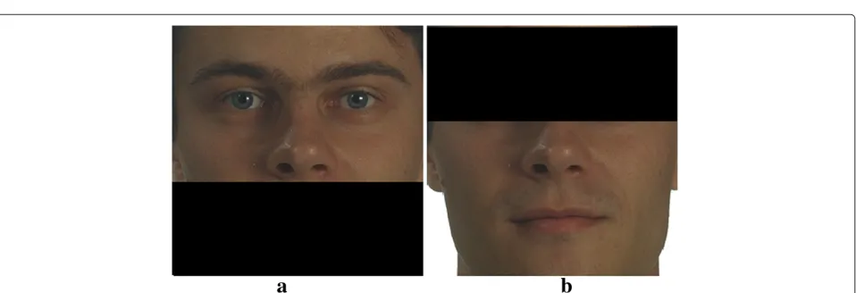
4.1 Occlusion cascade creation
Several occlusion cascades are created. Each one is in charge of a given occlusion type. To limit complexity, the case of two occlusion types is presented: bottom occlusion (called typeAin Figure 6a) and top occlusion (called type Bin Figure 6b). In occlusionA, the lower third of the face is considered as occluded. In occlusionB, the upper third of the face is considered as occluded.
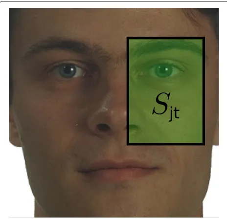
LetOI be the occluded area withI ∈ {A,B}, the set of occlusion configurations. Let Sjt be the region cov-ered by the subwindow associated with the weak classifier hjt (see Figure 7). For each occlusion type I, the set of available weak classifiers must be defined to build the associated occlusion cascade. A weak classifierhjtis avail-able for occlusionIif the areaSjtdoes not intersectOI. In other words, the associated subwindow is considered as occluded for the occlusionIif the areaSjtintersectsOI. ForI ∈ {A,B}, two setsHA andHB of available weak classifiers are defined:
HA= {hjt|Sjt∩OA= ∅}, (13) HB= {hjt|Sjt∩OB= ∅}. (14)
Based on these two sets, two McCascadesCAandCBcan be created.CAonly uses weak classifiers defined inHA. In the same way,CBonly uses weak classifiers defined in HB. Finally, thresholdsβjof both McCascades are fixed with the help of Algorithm 1.
4.2 Cascading with evidence
To combine the main cascadeCand the two occlusion cas-cadesCAandCB, the principle of cascading with evidence proposed by Lin et al. [7] is used. When a samplexmust be tested, it first goes through the main cascade. At levelj of this cascade, in addition to applying the strong classifier Hj, an additional feature vectorεj(x)is also computed:
εj(x)=(HjA(x),HjB(x)), (15)
where
HjI(x)= t|Sjt∩OI=∅
hjt(x)withI∈ {A,B}. (16)
The vectorεj(x)is called the evidence ofxat levelj. Equation 16 means thatHjI only involves weak classi-fiers over subwindows that do not intersect withOI. With the evidence vector presented in Equation 15, weak classi-fiers can now be defined as available or not depending on the occlusion encountered. Indeed, letxbe an occluded face example of typeAand suppose that the main cascade Crejects it at leveljbecauseHj(x) < αj. Before rejecting it, we check the evidence vector ofx. In particular, the major-ity ofH1A(x),. . .,HjA(x)should be positive, indicating that xis an occluded face of typeA. Based on this fact, weak classifiers that can handle occlusionA(i.e.,hjt verifying Sjt∩OA = ∅) are defined as available, andxcontinues the classification process with the McCascadeCAdefined on available weak classifiers. Generally speaking, if a sam-ple is occluded of type I and if this sample is rejected by the main cascade, this sample will be passed to the McCascadeCI. Note that with this principle of cascading with evidence, there is no explicit occlusion detection.
Figure 7Region covered by the subwindow associated to a weak classifier.The weak classifierhjtmust classify the regionSjt,
filled in green.
Using C, CA, and CB with the principle of cascading with evidence, we can detect occluded faces following the testing procedure described in Algorithm 3 whereCI represents the McCascade that can handle occlusionI. The testing procedure is also illustrated in Figure 8. All the above explanations remain valid with other types of occlusions. Note that the number of occlusions that can be handled only depends on the weak classifiers learned during the initial training. For example, if all the weak clas-sifiers learned are associated with subwindows located on the upper part of the face, it would be impossible to handle occlusions of typeB.
Algorithm 3:Detecting occluded objects with several McCascades combined with cascading with evidence
Input: An unknown examplex
Output: Label ofx:Face, Non-Face, ortype-I
occluded Face
1 if xgoes throughCthen returnFace;
2 if xis rejected at level j and all HjI(x) <0then return
Non-Face;
3 DispatchxtoCIifHjI(x) >0 andji=1HiI(x)is the largest;
4 if xgoes throughCIthen
5 returntype-I occluded Face;
6 else
7 returnNon-Face;
8 end if
5 Application to multiview face detection
In this section, we are interested in the detection of faces with rotation-off-plane (ROP) angles. Examples of such faces are exposed in Figure 9. Upright face detectors are robust to slight ROP angles (they can usually detect faces turned up to±20°). Detection of faces with bigger ROP angles need specific solutions. Most of the existing meth-ods adopt the view-based approach: several classifiers are trained and then combined to get a multiview face detector [1,12,13]. In such an approach, each classifier is trained to detect faces with ROP angles in a given range which means that multiple training is necessary. To avoid these multiple trainings, we propose to create a classi-fier that can detect faces in a pose different than the one learned.
5.1 Detecting faces with ROP angle
Our solution is composed of an upright face detector that we modify to be able to detect faces with a given ROP angle. To incorporate the fact that faces may have out-of-plane rotations, we propose to adjust all the sub-window positions. Our idea is illustrated in Figure 10c. Figure 10a shows three interesting subwindows used to detect upright faces. In Figure 10b, we represent the same subwindows on a face turned 45°. The three subwindows are not anymore informative. To alleviate this problem, we can modify the position of the three subwindows (see Figure 10c). Note that the position modification can lead to a modification of the subwindow size (see the yellow subwindow) or the disappearance of some subwindows (see the red subwindow).
To modify a subwindow position, we propose to use the three-dimensional (3D) transformation which exists between an upright face and the same face in another pose. In our case, these transformations are the set of rota-tions around thex-axis andy-axis. To simulate a rotation, we need a 3D face model. Building an accurate 3D face model requires at least two images per face. As our inten-tion is to avoid gathering images other than upright faces, we decide to represent a face with the simplest model: an ellipsoid. The idea is then to place each subwindow on the ellipsoid, turn the ellipsoid, and finally get back all the new subwindows positions. Let us consider a point pi1=(u1v1)T of an image of sizew×w(the same size as training images) whose coordinates are expressed in the image coordinate systemCSi. The process to compute the position of this point after a rotation defined by an angle ofθxaround thex-axis and an angle ofθyaround they-axis is made up of the following three steps:
Figure 8Testing procedure of the association of a cascade and a McCascade.Example x is first processed by initial cascadeCand then dispatched to McCascadeCAto finally be detected as typeAoccluded face.
the help of the ellipsoid equation expressed inCSi (see Figure 11a):
(u−u0)2
a2 +
(v−v0)2
b2 +
(w−w0)2
c2 =1, (17)
whereuo=w/2,vo=w/2, andwo=0anda, b, and c are the ellipsoid’s parameters.
2. We expressPi1in the coordinate systemCSewhose origin is the ellipsoid center. This gives us thePe1 point: ⎡ ⎢ ⎢ ⎣ ˜ x1 ˜ y1 ˜ z1 ˜ d1 ⎤ ⎥ ⎥ ⎦= ⎡ ⎢ ⎢ ⎣
1 0 0 −w/2 0 1 0 −w/2 0 0 1 0 0 0 0 1
⎤ ⎥ ⎥ ⎦ ⎡ ⎢ ⎢ ⎣ u1 v1 w1 1 ⎤ ⎥ ⎥
⎦, (18)
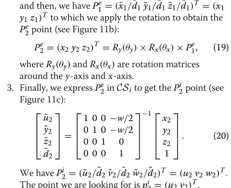
and then, we havePe1=(x˜1/˜d1y˜1/d˜1z˜1/˜d1)T =(x1 y1z1)Tto which we apply the rotation to obtain the Pe2point (see Figure 11b):
Pe2=(x2y2z2)T =Ry(θy)×Rx(θx)×P1e, (19)
whereRy(θy)andRx(θx)are rotation matrices around they-axis and x-axis.
3. Finally, we expressPe2inCSito get thePi2point (see Figure 11c): ⎡ ⎢ ⎢ ⎣ ˜ u2 ˜ y2 ˜ z2 ˜ d2 ⎤ ⎥ ⎥ ⎦= ⎡ ⎢ ⎢ ⎣
1 0 0 −w/2 0 1 0 −w/2 0 0 1 0 0 0 0 1
⎤ ⎥ ⎥ ⎦
−1⎡
⎢ ⎢ ⎣ x2 y2 z2 1 ⎤ ⎥ ⎥
⎦. (20)
Figure 9Example of faces with rotation-off-plane angles around they-axis.The face is turned 90° in(a), 67.5° in(b), 45° in(c), and 22.5° in(d).
To know the position of a subwindowrjtafter a rotation, we apply the above process to the top left corner and to the bottom right corner ofrjt. The problem is that some subwindows can disappear (as shown in Figure 10c with the subwindow ofh3in red). If a subwindowrjtdisappears, then the associated weak classifierhjt becomes unavail-able. By applying this rule to all the subwindows, the set of available weak classifiers can be defined and an associated McCascade can be built. Hence, creating a classifier that can detect non-upright faces calls for three steps:
1. Modifying the position of all subwindows using an ellipsoid model,
2. Defining the set of available weak classifiers by checking that their associated subwindows do not disappear after rotation, and
3. Creating the McCascade using available weak classifiers.
5.2 A multiview system
The solution presented in the last section aims to detect faces with a given ROP angleθy. When faces with a ROP angle in a range [−θymin,+θymax] are to be detected, one solution is to combine several detectors. Each one is spe-cialized in detecting faces with a given ROP angleθy. In
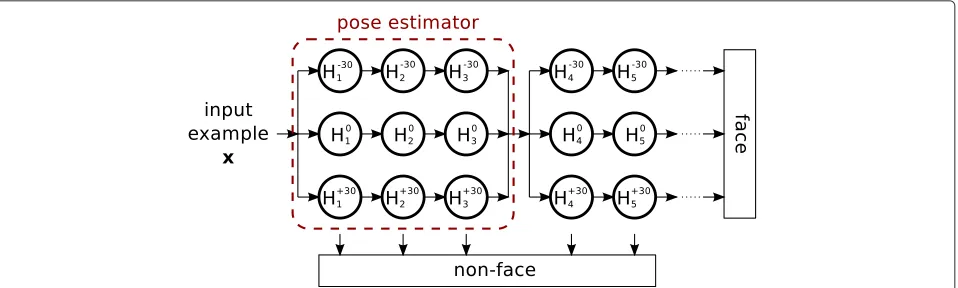
practice, it is generally assumed that each detector can detect faces in the range [θy −15,θy + 15]. For exam-ple, if the total range is [−45,+45], three detectors must be used: an upright face detectorH0, a detector of faces turned +30°H+30, and a detector of faces turned−30° H−30. DetectorsH+30 andH−30 are created by modify-ing all subwindow positions byH0. To combine the three detectors, the solution proposed by Huang et al. [14] is applied. It is illustrated in Figure 12. To speed up the clas-sification process, a pose estimator is used. For an input examplex, this estimation consists in applying the first three levels of every detector tox. Then, the classification process continues with the detector that acceptsxwith the highest classification score. The pose estimation function is defined by:
pose(x)= argmax θy∈{−30,0,30}
H3θy(x)
. (21)
Note that the system used to combine the three detec-tors can be extended to get a face detector robust to pose and to occlusion. Indeed, using this system, several occlusion cascades (presented in Section 4.1) and several pose-specific detectors (presented in Section 5.1) can be combined.
Figure 11Rotation process of a point using an ellipsoid.(a)The image pointpi1=(u1,v1)is associated with the pointPi1=(u1,v1,w1)on the ellipsoid using the ellipsoid equation.(b)Pi1is expressed in the ellipsoid coordinate system which gives the pointPe1. The rotated pointPe2is computed using rotation matrices.(c)Pe2is expressed in the image coordinate system which gives the pointPi2=(u2,v2,w2)and the image point
pi2=(u2,v2).
6 Experiments
This section presents the experiments achieved in order to (1) evaluate the performances of McCascade compared to the naive approach and (2) evaluate the McCascade algorithm for two concrete applications: occluded face detection and multiview face detection. In these experi-ments, upright face detectors are similar to the system of Tuzel et al. [15]: covariance matrices are used as features [16], and the learning algorithm is a cascade of LogitBoost [10]. Weak classifiers are linear functions that are learned from a set of feature vectors. A feature vector is derived from a covariance matrix by taking its upper triangular part. The only difference with the system [15] is that we assume that a feature vector lies on a vector space (in [15], a feature vector lies on a Riemannian manifold).
The first part of the experiments related to McCascade performance (Sections 6.2 and 6.3) are done with an upright face cascaded detector of three levels with 5, 10, and 25 weak classifiers, respectively. Positive examples
come from thelabeled upright faces in the wilddatabase [17], and negative samples were generated from 1,310 images containing no face. A total of 4,000 positive exam-ples and 8,000 negative examexam-ples are used to train each cascade level. The second part of the experiments related to applications (Sections 6.4, 6.5, and 6.6) are done with an upright face detector of nine levels. This detector is noted C. Each level was trained with 5,000 positive examples and 5,000 negative examples. Each level was designed so that a detection rate of at leastdmin=0.998 and a false-positive rate of at most fmax = 0.5 were achieved on training examples. The positive examples again come from the labeled upright faces in the wild database, and negative samples were generated from 2,500 images containing no face. The FLANN library [18] is used to perform nearest neighbor searches (used inPknn andPcomb). The test database is the CMU frontal face test A which con-sists of 42 images showing 169 upright faces with varied background [19].
In the first part of the experiments, receiver opera-tor characteristic (ROC) curves are used to evaluate and compare performances, and all performances exhibited are raw, i.e., the post-processing step of merging mul-tiple detections is not taken into account here. This means that the false-positive rate can be reduced with this post-processing step without modifying the true-positive rate. When multiple detections occur for the same person, only the one with the highest classifica-tion score is kept. The others are simply ignored. In the second part of the experiments, free ROC(FROC) curves are used, and multiple detections are merged. Con-trary to the ROC curve which plots detection rate versus false acceptance rate, the FROC curve plots the detec-tion rate versus the number of false-positives and is more suited to evaluate performances of an object detector in specific applications. Different experiments were con-ducted to evaluate the different aspects of our method. In Section 6.2, we test the three proposed cost functions TP_cost, FP_cost, and FP_TP_cost used in the computa-tion of McCascade’s thresholds. Then, Seccomputa-tion 6.3 deals with the evaluation of the different strategies used to estimate posterior probability: Pboost, Pknn, and Pcomb. After these two series of experiments, we apply our method to two specific applications: detecting faces occluded by a scarf or sunglasses (see Section 6.4) and
detecting faces in a pose different than the one learned (see Section 6.5).
6.1 Good detection criterion
Building ROC or FROC curves requires computing true-positive rates and false-true-positive rates. A criterion must be defined to decide if a given detection is a true-positive or a false-positive. The criterion used in these experiments is defined in the overlap between the detection and the ground truth. It was proposed by Yao and Odobez [20]. The overlap is computed with theFmeasureFoverlap:
Foverlap(GT,D)= 2ρπ
ρ+π where ρ=
|GT∩D| |GT|
and π = |GT∩D| |D| .
(22)
ρstands for the precision area andπ for the recall area. GT is the ground truth area, andDis the detection area. The operator|R|is the number of pixels in the areaR. A detection matches with ground truth ifFoverlap>0.5.
6.2 Evaluation of threshold estimation strategies
In this first part, we evaluate the influence of the cost func-tion in thresholdβj estimation when a given proportion
of weak classifiers is missing. We chose to consider 50% and 60% of missing weak classifiers because these rates are realistic in occluded face detection. Given a missing weak classifier rate, we randomly create two sets of weak classifiers per level to be considered as unavailable. For example, consider the level 2 of the classifier which has ten weak classifiers. If 60% of the weak classifiers are miss-ing, then 6 weak classifiers must be selected as unavailable. For each of the two sets of unavailable weak classifiers, we randomly select six weak classifiers to be considered as unavailable. These two sets could be{h21,h22,h23,h24, h27,h29}and{h22,h23,h25,h26,h27,h28}. Given the sets of the three levels, there are 2×2×2 =8 possible con-figurations to test resulting in eight ROC curves. Means and standard deviations are then computed to produce the final ROC curve. For each configuration, thresholds are first computed and the resulting classifier is applied to the test database. This test process is repeated for each cost function associated to each posterior probability compu-tation strategy:Pboost, Pknn, and Pcomb. For the last two strategies, we fix the number of neighborskat 3. All the ROC curves are available in Figure 13. In all the curves, the cost function TP_cost produces a classifier that out-performs the other classifiers produced with FP_cost and FP_TP_cost.
ROC curves are useful in evaluating the overall per-formance of a classifier. When we train a classifier, this presents a given true-positive rate and a given false-positive rate which should be consistent with the appli-cation targeted. In face detection, we are interested in having a high true-positive rate and a low false-positive rate. This is why, in addition to ROC curves, we present the false-positive rate, noted FP, and the true-positive rate, noted TP, of classifiers produced by the three cost func-tions. Results for a missing rate of 50% can be found in Table 1, while results for 60% are available in Table 2. In these tables, we also print the mean number of levels evaluated per negative example, noted nlevel. This cri-terion reflects the impact of the cost function on the execution time of the classifier. Indeed, a high number of evaluated levels per negative example will bring a high execution time. In both tables, we print in italics the cost function that provides the most consistent perfor-mance. As expected, the use of cost functions FP_cost and FP_TP_cost involves low false-positive rates but also involves low true-positive rates (some of them lower than 10%), which means that these classifiers do not have a practical value. Furthermore, the impact on the mean number of evaluated levels is not very significant: we note an increase of about 7% between the cost function TP_cost and the two others. These experiments prompt us to keep the cost function TP_cost because FP_cost and FP_TP_cost tend to decrease the true-positive rate and the overall performance.
Table 1 Evaluation of cost function used to compute thresholdsβjwhen 50% of weak classifiers are missing
k Cost function FP TP nlevel
×10−3
Pboost
-TP_cost 3.21 0.88 1.61
FP_cost 0.066 0.1 1.48
FP_TP_cost 0.08 0.15 1.48
Pknn 3
TP_cost 5.56 0.95 1.29
FP_cost 0.14 0.52 1.26
FP_TP_cost 0.17 0.44 1.29
Pcomb 3
TP_cost 5.43 0.95 1.62
FP_cost 0.006 0.12 1.48
FP_TP_cost 0.03 0.24 1.48
Three evaluation terms are exposed: the false positive rate, the true positive rate
and the mean number of evaluated levels per negative example notednlevel.
6.3 Performance of the posterior probability estimation
In this section, we evaluate the three strategies to estimate posterior probabilities proposed in Section 3.3: Pboost, Pknn, andPcomb. The evaluation methodology is the same as the previous section (same cascaded detector, same test database, same missing rate). Here, the cost function used to compute thresholds is TP_cost. Five configura-tions are compared: (1) ‘CascadeF’ is the initial cascade with the full set of weak classifiers (can be seen as an upper bound), (2) ‘CascadeA’ is the naive approach pre-sented in Section 3.1 where the initial cascade is only used with available weak classifiers, (3) ‘McCascade + Pboost’ is a McCascade used with available weak clas-sifiers where posterior probabilities are computed with Pboost, (4) ‘McCascade + Pknn’ is a McCascade used with available weak classifiers where posterior probabilities are computed with Pknn, and (5) ‘McCascade + Pcomb’ is
Table 2 Evaluation of cost function used to compute thresholdsβjwhen 60% of weak classifiers are missing
k Cost function FP TP nlevel
×10−3
Pboost
-TP_cost 8.4 0.95 1.64
FP_cost 0.058 0.06 1.48
FP_TP_cost 0.17 0.29 1.49
Pknn 3
TP_cost 8.25 0.96 1.32
FP_cost 0.15 0.56 1.26
FP_TP_cost 0.28 0.58 1.32
Pcomb 3
TP_cost 11.9 0.97 1.67
FP_cost 0.005 0.11 1.48
FP_TP_cost 0.16 0.49 1.5
Three evaluation terms are exposed: the false positive rate, the true positive rate
a McCascade used with available weak classifiers where posterior probabilities are computed with Pcomb. When Pknn andPcomb are used, only the best results are plot-ted (k = 7 forPknn andk = 3 for Pcomb). The results can be found in Figure 14. In both cases, the McCascade structure improves the performance. The most interest-ing results are obtained whenPknn andPcomb are used. In that case, the true positive rate increases from 10 to 30% when 50% of weak classifiers are unavailable. When 60% of weak classifiers are unavailable, the improvement is even higher: from 20% to 60%. In both cases, the proposed method outperforms the naive approach. More-over, McCascade is really more stable than the naive approach (see standard deviations in each curve) which ensures good performance in every case. Finally, the pro-posed method does not suffer from the additional 10% of unavailable weak classifiers. Even if Pknn and Pcomb are close in terms of performance, we note thatPknnis slightly better.
The influence of the number of neighbors in the McCascade coupled with the strategyPknncan be found in Figure 15. In both cases,k = 7 gets the best perfor-mances, but k = 3 should be preferred as it provides similar performance and lower computational cost. In all the following experiments, the McCascade is used with thePknnstrategy andk=3.
An additional result is given in the Figure 16 where 30% of the weak classifiers are missing. Below this rate of 30%, the naive approach and the McCascade get close performances. However, when at least 30% of the weak classifiers are missing, using a McCascade becomes interesting. Indeed, it can be noted in Figure 16 that a McCascade with the strategy Pknn increases the true-positive rate up to 30% compared to the naive approach.
6.4 Occluded face detection
In this section, we evaluate the performance of McCascade coupled with the principle of cascading with evidence in a specific application: detecting faces with top occlusions (like sunglasses) or bottom occlusions (like a scarf ). We only consider these two types of occlusions for two reasons. The first is that we are working in a video surveillance context in which these two types of occlusions are often encountered. The second reason is that a public database with these two types of occlusion is available: the AR database.
6.4.1 Evaluation on the AR database
The AR database [21] is used first. In particular, we use the 765 images of faces occluded by a scarf and the 765 images of faces occluded by sunglasses. The classifier used here is the upright face detector of nine levels. Using this cascadeC, we build a McCascadeCAthat can handle bot-tom occlusion and a McCascadeCBthat can handle top occlusion. Also, a detector that associatesC,CA, andCB with the principle of cascading with evidence is created. This detector will be noted ‘McCascades + evidence’ in the results. The McCascadeCAhas, on average, 42% unavail-able weak classifiers per level. The McCascadeCBhas, on average, 46% unavailable weak classifiers per level.
Two scenarios are tested:
• Scenario 1. We consider images of faces occluded by a scarf, and we then compare (1) the cascadeC, (2) the McCascadeCA, and (3) the detector McCascades + evidence.
• Scenario 2. We consider images of faces occluded by sunglasses, and we then compare (1) the cascadeC, 2) the McCascadeCB, and (3) the detector McCascades + evidence.
Figure 15Influence of the number of nearest neighborskin the strategyPknn.In(a), 50% of weak classifiers are missing, and in(b), 60% of weak classifiers are missing.
For all scenarios, FROC curves are computed. To create the FROC curve of a cascaded detector, several thresh-old values are tested for the last level which results in corresponding points of detection rate and number of false-positives. To get more points (points with a higher detection rate and a higher number of false-positives), the last level must be removed, and then different thresholds for the new last level are tested. This procedure con-tinues until enough points are collected. When several cascades are associated (e.g., in the system ‘C+CA+CB+ evidence’), creating a FROC curve is not straightforward because each cascade has its own thresholds. To alleviate this problem, we use the idea proposed by Viola and Jones in [22]. To create FROC curves from multiple cascades, thresholds are simultaneously modified in all cascades. In the same way, layers are simultaneously removed in all cascades.
Figure 16A McCascade becomes interesting when at least 30% of the weak classifiers are missing.
The FROC curve of scenario 1 is available in Figure 17. The McCascadeCA(noted ‘McCascade’) greatly improves the detection rate (up to 30%). The drawback of CA is that it is designed to detect faces with bottom occlusions. When the encountered occlusion is unknown (top or bottom), the detector McCascades + evidence can be used, and Figure 17 shows that its performances are close to the ones ofCA.
The FROC curve of scenario 2 is available in Figure 18a. On faces occluded by sunglasses, the initial cascade and the proposed solutions (the detector CB and the detec-tor McCascades + evidence) expose very poor results. The poor results in scenario 2 are due to a limitation in our solution: the fact that each weak classifier does not have the same performance. Several works on face detec-tion noticed that learned weak classifiers often rely on the
Figure 18Limitation of the proposed solution.(a)Comparison of the initial cascadeC(noted Cascade), the McCascadeCB(noted McCascade), and the association ofC,CA, andCBwith the principle of cascading with evidence (noted McCascades + evidence) on faces occluded by sunglasses.(b)Performance map of all the weak classifiers in the initial cascade. Note that most of the performance is located on the upper part of the face (best seen in color).
upper part of the face to make a decision because the eye area is very discriminative. When our upright face detec-tor was trained, we noticed the same phenomenon: most of the weak classifiers are located on the upper part of the face, and they are more powerful than the weak classifiers located on the lower part of the face. This fact can be seen in Figure 18b which represents a performance mapMof all the weak classifiers in the initial cascade. To build this map, we first initialize all values to zero. Then, for all the weak classifierhjt, we compute its classification rateCRjt (rate of well-classified positive and negative examples), and we updateMwith:
M(x,y)=M(x,y)+CRjt ∀(x,y)∈Sjt⊂M. (23)
Finally, we normalize all the values between 0 and 1. Based on this map, we understand that our method fails on faces occluded by sunglasses because, in this sce-nario, we only use weak classifiers located on the lower part of the face which are too weak to ensure good performance.
In scenario 2, the existing solutions such as [7] will exhibit better results. Indeed, a specific classifier will be trained to detect faces with top occlusions. In scenario 1, it is interesting to compare our system with [7]. Rather than building the complete system described in [7], a specific classifier was trained to detect faces with bottom occlu-sion. This specific classifier is close to cascadeC, except that all the learned weak classifiers are located on the area that it is not occluded. This specific classifier is then com-pared with the McCascadeCA. Results can be found in the Figure 19. Except with a very low number of false-positives, the specific classifier gets a higher detection rate (up to 10%).
6.4.2 Evaluation in real-life scenario
A test is also done in a real-life scenario. A camera is placed on a pole to film a group of 15 persons. Some of them have their face occluded by a scarf, coat, or hood. Examples of images from the sequence are available in Figure 20. There is a small angle (around 20°) between the optical axis of the camera and the ground to imitate conditions of a video surveillance context.
Three detectors are applied to this sequence:
• Upright face detectorC. It is noted ‘FDcov’ in the
results.
• Detector that associatesC,CA, andCBwith the principle of cascading with evidence. It is noted ‘FDcov+ occlusion’ in the results.
• Upright face detector of the OpenCV library (the file
Figure 20Images from a realistic sequence.A group of 15 persons are filmed by a camera on a pole. Some of them have their face occluded by a scarf, coat, or hood. The 15 persons can be seen in(a),(b), and(c).
haarcascade_frontalface_alt_tree.xml
is used). This detector is the implementation of the solution of Lienhart et al. [23]. This classifier is a cascade of boosted classifiers. Haar features are used. It is noted ‘FDhaar’ in the results.
The detector FDhaar just gives output detections. The classification score of each detection is not known. This detector is applied first on the sequence. Then, with the help of ground truth, the detection rate per person is computed. The number of false-positives nbFPhaaris also noted. The other two detectors are then applied to the sequence. The rejection thresholds of the two detectors are modified so that they obtain nbFPhaarfalse-positives. Then, the detection rate per person is computed. The results are available in Figure 21. The red line is the aver-age detection rate of the detector FDhaar. The yellow line is the average detection rate of the detector FDcov, and
Figure 21Comparison of FDhaar, FDcov, and FDcov+ occlusion on a realistic sequence.Each number on the horizontal axis is associated to a person in the sequence. The vertical axis is the detection rate. The red line is the average detection rate of FDhaar. The yellow line is the average detection rate of FDcovand the green line is the average detection rate of FDcov+ occlusion.
the green line is the average detection rate of the detector FDcov+ occlusion. The worst performances are obtained with FDhaarwith 38% true-positive rate. FDcovgets a 47% true-positive rate. The best performances are achieved by FDcov + occlusion with a true positive rate of 75%. Moreover, we note that FDhaar does not detect persons 11, 12, and 14. They are detected by the other two clas-sifiers. Detection examples of these persons are given in Figure 22.
6.5 Multiview face detection
In this part of the experiments, the boosted McCas-cade algorithm has been applied to another specific application: detecting faces in different poses using an upright face detector. The FERET database [24] was used to evaluate the system. We test our method on faces turned 22.5°, 45° and 67.5°. For each angle, all the sub-window positions are first adjusted using the procedure described in Section 5.
6.5.1 Ellipsoid parameters
To modify the subwindow positions, parametersw,a,b, andcmust be fixed. Parameterwcorresponds to the size of the training images which is 24 in our case. To fix ellip-soid parameters a, b, and c, we do an exhaustive search and keep the parameters, giving the best results on vali-dation sets from the FERET database. Two valivali-dation sets were created: one for the angle 22.5° and one for 45°. For each angle, we keep half of the images to fix the ellip-soid parameters. The other half is used to evaluate the complete system. For each parameter value(ai,bi,ci), we apply the following methodology:
1. Based on the upright face classifier, we create two classifiersC22.5andC45by adjusting all the subwindow positions using ellipsoid parameters (ai,bi,ci). Subwindows that disappear are handled by the naive approach presented in Section 3.1, i.e., associated weak classifiers are simply ignored. 2. C22.5is applied to the validation set of images of faces
Figure 22Persons that are not detected by FDhaar.In(a), the person is occluded by a hood. In(b), the glasses and the beard make the person difficult to detect. In(c), the person is occluded by a scarf.
the area under ROC curve is computed which gives auc22.5i (auc is a criterion to compare ROC curves: the higher it is, the better the ROC curve). UsingC45, we also get auc45i .
3. Finally, the overall value auci=auc22.5i +auc45i is computed.
Parameters with the best value auciwere kept. We found thata = 2.0∗w/2,b = w. andc = w/2 give the best results.
6.5.2 Modification of subwindow positions
Here, the use of an ellipsoid to modify subwindow posi-tions is evaluated. Three detectors are built:
• C22.5is a detector of faces that turned22.5°, • C45is a detector of faces that turned45°, and • C67.5is a detector of faces that turned67.5°.
Each one is built fromCby modifying subwindow posi-tions. Subwindows that disappear are handled by the naive approach. These detectors are then applied to images
from the FERET database. The results are available in Figures 23 and 24. In each curve, the upright face detec-torCis noted ‘Cascade’. DetectorsC22.5,C45andC67.5are noted ‘MaCascade’ (for cascade with multiview adapta-tion). On faces turned 22.5°, the improvement is slight because the appearance of such faces is still close to the appearance of upright faces. The improvement is greater on faces turned 45°. Indeed, the detection rate increases from 30% to 40%. Finally, we see that the detection of faces turned 67.5° can be seen as a limitation of the proposed method. A detection rate increase (up to 60%) only occurs when the number of false-positives becomes high (>30). This limitation comes from the step of adjusting the sub-window positions:
1. The subwindow position modification should compensate the modified appearance of a turned face of an angleθy. When the angleθyincreases, it becomes much more difficult to compensate the modified appearance as the modification becomes stronger and stronger.
Figure 24Performances of different detectors on faces turned
67.5°.The detector Cascade is the upright face detector. The detector MaCascade is built from the upright face detector and aims to detect turned faces. Subwindow positions are modified and unavailable weak classifiers are handled by the naive approach. The detector MaMcCascade is the same detector as MaCascade except that unavailable weak classifiers are handled with a McCascade. The detector MaMcCascade multiview is a multiview system that combines three MaMcCascades: one for the angle 22.5°, one for 45°, and one for 67.5°.
2. In Section 5, we explain that some subwindows can disappear due to rotation. In fact, the number of subwindows that disappear increases with the angle θy. This loss impacts the initial performance.
6.5.3 Association with a McCascade
The three detectors of the previous sectionC22.5,C45, and C67.5have some unavailable weak classifiers:
Figure 25Comparison of the classifier MaMcCascade and the specific cascade on faces turned45°.
Table 3 Mean detection time on faces turned 45°
Classifier Mean time Minimum time Maximum time
(ms) (ms) (ms)
Cascade 234±46 196 593
MaMcCascade 296±96 201 663
Times for the initial upright face detector (noted Cascade) and for the MaMcCascade system are compared.
• C22,5has, on average, 18% unavailable weak classifiers per level.
• C45has, on average, 27% unavailable weak classifiers per level.
• C67,5has, on average, 44% unavailable weak classifiers per level.
Unlike using the naive approach to handle these unavail-able weak classifiers, it could be interesting to modify the cascade structure into a McCascade. In this section, the structure of the three detectors is changed into a McCascade. The strategyPknnis used withk = 3 neigh-bors, and thresholds βj are fixed using the cost func-tion TP_cost. In Figures 23 and 24, these detectors are noted ‘MaMcCascade’. On faces turned 22.5° and 45°, the improvement compared to the naive approach is slight (increase of the detection rate from 2% to 5%). The impact of using a McCascade is greater on faces turned 67.5°. Indeed, contrary to the naive approach, the McCascade allows for the detection rate to be improved with only a few false-positives. However, performances remain lim-ited. For example, 55% of faces are detected with 12 false-positives, while this rate is 90% when faces are turned 22.5° and 45°.
Detecting faces turned 67.5° with the existing solutions such as [1,12,13] will exhibit better results. Indeed, a spe-cific classifier will be train to detect faces turned 67.5°. When faces are turned 45°, it is interesting to compare the system MaMcCascade with a specific classifier. Thus, a specific classifier was trained using the same train-ing parameters as the cascadeC, except that the positive images were extracted from the FERET database. A total of 132 images of faces turned 45° were extracted to train the specific classifier (these images are not used during the testing stage). Results can be found in Figure 25 where we
Table 4 Mean detection time on faces occluded by a scarf
Classifier Mean time Minimum time Maximum time
(ms) (ms) (ms)
Cascade 375±43 272 610
McCascade + evidence 468±63 335 758