http://www.sciencepublishinggroup.com/j/ijecec doi: 10.11648/j.ijecec.20190501.13
ISSN: 2469-8040 (Print); ISSN: 2469-8059 (Online)
Optimal Placement of an Unified Power Flow Controller in a
Transmission Network by Unified Non Dominated Sorting
Genetic Algorithm-III and Differential Evolution Algorithm
Oloulade Arouna
1, Moukengue Imano Adolphe
2, Fifatin François-Xavier
3,
Ganye Sewlan Amedee Arcadius
1, Badarou Ramanou
3, Vianou Antoine
4, Tamadaho Herman
11
Electrotechnic, Telecommunications and Informatics Laboratory (LETIA), University of Abomey-Calavi, Abomey-Calavi, Benin 2
Laboratory of Electrical Engineering, Electronics, Automation and Telecommunications, University of Douala, Douala, Cameroon 3
Polytechnic School of Abomey-Calavi, University of Abomey-Calavi, Abomey-Calavi, Benin 4
Laboratory of Thermophysic Characterization of Materials and Energy Mastering, University of Abomey-Calavi, Abomey-Calavi, Benin
Email address:
To cite this article:
Oloulade Arouna, Moukengue Imano Adolphe, Fifatin François-Xavier, Ganye Sewlan Amedee Arcadius, Badarou Ramanou, Vianou Antoine, Tamadaho Herman. Optimal Placement of an Unified Power Flow Controller in a Transmission Network by Unified Non
Dominated Sorting Genetic Algorithm-III and Differential Evolution Algorithm. International Journal of Electrical Components and Energy Conversion. Vol. 5, No. 1, 2019, pp. 10-19. doi: 10.11648/j.ijecec.20190501.13
Received: May 17, 2019; Accepted: June 17, 2019; Published: July 2, 2019
Abstract:
The interconnected transmission network of the Benin Electric Community (CEB) presents excessive losses that will increase further by 2025 and severely degrade the power quality supplying. This paper presents the quarto-criterion optimization of the positioning of a UPFC in the CEB's HTB network by U-NSGA III and DE. The positioning of an UPFC on line 3 and node 6 of this network has qualitatively improved the technical performance of this transmission network with an optimal installation cost of US $ 13126657.03. The hypervolumes of the two calculated methods showed that the U-NSGA-III is more accurate in terms of trend toward global solutions than DE. These convincing results confirm the performance of the U-NSGA-III method compared to the DE which also resulted in results close to those obtained by the U-NSGA-III with more or less narrow difference.Keywords:
U-NSGA-III, CEB, Hypervolume, UPFC, DE1. Introduction
The disintegration of the traditional electrical system associated with the strong environmental constraints that limit the construction of new power lines are driving transmission system operators to exploit existing transmission networks to their limits of stability. In this new context, the existing High Voltage Category B (HVB) installations are more and more solicited and involve enormous losses, risks of voltage instability and power capacity limits violation. These limits violation are generally manifested by causing harmful tripping. The power transformers installed in the high voltage substations are equipped with load regulators that are no longer able to
this network would be an economically and technically attractive alternative for solving the voltage instability and loss operating problems in this high voltage transmission network of CEB.
The UPFC is a shunt-series FACTS type whose role is to contribuate to the improvement of static and transient voltage stability and phase angle regulation. It allows the control of power flow in transmission network. Interconnected transmission networks are characterized by several transmission lines and several nodes. The choice of the location of an UPFC in a transmission network is a combinatorial optimization problem. The resolution of this type of problems require metaheuristics generally provide global optimal solutions in contrast to deterministic methods [2]. Given the growing interest in this topic of FACTS optimal positioning in a transmission network today, several authors have focused on optimizing FACTS' positioning in transmission networks to reduce losses. improve stability and voltage profile.
W. Chang has used the mixed integer linear programming approach to position an UPFC in a network to maximize transit capacity [3]. T. Kurshaid has used an approach based on reactive loss sensitivity index for optimal positioning of an UPFC in a meshed transmission network [4]. This technique involves placing the UPFC on the line with the most positive sensitivity index. Navani et al have proposed a method based on the active loss sensitivity index and the loss performance index to position an UPFC in the IEEE-14 bus transmission network [5]. Stakshi Singh has also used the loss sensitivity index to choose the optimal location of the UPFC to reduce losses on the transmission lines [6]. These so-called analytical methods are simple to use but precision is not guaranteed in the results. So several researchers prefered metaheuristic methods. Shah has used real coded genetic algorithms to place several types of FACTS such as: UPFC, Static Var Compensator (SVC) and Thyristor Controlled Series Compensator (TCSC) into the IEEE-30 network. These have made possible to increase the power flow capacity of the lines [7]. E. Ghahremani has developed a Genetic Algorithm (GA) based approch to select nodes for simultaneous placement of UPFCs, SVCs, TCSCs and Thyristor Controlled Voltage Regulator (TCVR) in a 57-node transmission network [8]. Bhandakar has also used GA for optimal placement of an UPFC and HPFC in a transmission network [9]. Made Wartana has used the Nondominated Sorting Genetic Algorithm-II (NSGA-II) to place an UPFC that has improved transmission capacity and reduced losses in a transmission network [10]. Mahdi M. et al have also used NSGA-II to do the optimal positioning of FACTS devices such as: UPFC, SVC and TCSC to reduce losses and risks of voltage instability [11]. Shaheen et al have presented an approach based on Differential Evolution (DE) to place an UPFC in transmission network like IEEE-14 and IEEE-30 [12]. V. Kumar and Srikanth have developed a hybrid method based on Artificial Bee Colony and Gravity Search Algorithm to make optimal positioning
of UPFCs in a transmission network [13]. In this work, the NSGA-III-inspired U-NSGA-III to place an UPFC in the CEB's interconnected transmission network.
Let’s begin our approch by presenting CEB’s transmission network and his state.
2. CEB’s Power Transmission Network
The CEB’s transmission network supplying the territories of Benin and Togo is obsolescent. Indeed, most of the HTB / HTA transmission lines and transformers are built since 1973, date of creation of this bi-state structure. Today, the electrical load in this power network have grown dramatically in both countries due to the development of housing and industrialization. The load’s peak on the network of Benin is estimated at 240MW, and 200MW in Togo. Some transmission lines have reached and exceeded their nominal transmission capacity and as result are causing excessive losses. Some transformers are obsolete and generate malfunctions that cause frequent interruptions in the supply of electrical energy. The Nangbéto hydroelectric power plant with a capacity of 32.8 MW x 2 has been built since 1973. The plant’s facilities are virtually damped and no longer allow optimal use of all the power available. In 2016, a modernization of its voltage and speed regulation systems improved the efficiency of this plant by at least 20%. The CEB import energy from the Volta River Authority (VRA) in Ghana and the TCN in Nigeria. The impossibility of coupling this two voltage leads the CEB’s operators to use his network isotage with respect to each of the networks of the two countries (Nigeria and Ghana). This situation requires some manoeuvre on the network to adapt it to the loads and production constraints. These manoeuvre result in interruptions that reduce the availability of the power supplying. Energy losses are increasing year by year due to the inadequacy of certain lines in relation to transit and overloads on certain equipment.
3. Power Flow Calculation
X / R ratios are high for power transmission networks. Among the power flow calculation methods, the method of Newton-Raphson and taking into account the speed of its convergence is suitable for the calculation of load flow in the transmission networks. As part of this study an algorithm based on the Newton-Raphson method have been developed to calculate the load flow in the CEB network.
3.1. Newton Raphson‘s Method
Newton Raphson's method is based on the Taylor series development limited to the first terms. The algorithm developed and implemented for this purpose in MATLAB is declined in the algorithm 1.
Algorithm 1: Newton-Raphson algorithm. Input: Branch parameters.
Source and load power values (P and Q). Initial values of voltage V and angle θ. Tolerance ε and number of iteration Ni.
1. Form the admittance matrix. 2. k ← 0.
3. while (max|∆P | >ϵ OR max|∆Q| >ϵ) AND (k < Ni). 4. Calculate the elements of the Jacobian matrix. 5. Calculate ∆V and ∆θ.
6. Update V et θ.
V k 1 ← V k ∆V k (1) θk 1 ← θk ∆θk (2) 7. k ← k + 1.
End.
3.2. Application of the Newton Raphson Algorithm for the Calculation of the CEB Network
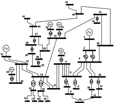
The CEB network, whose diagram is shown in Figure 1, consists of 42 nodes. It also consists of 40 lines and 16 power transformers with several voltage levels (330kV, 161kV and 63kV).
Figure 1. Single line diagram of the CEB's interconnected network.
Taking into account the average growth rate load in the CEB network which is 4.9% [14] based on CEB statistics, we applied the code developed under the MATLAB environment to compute the load flow in the network of the CEB by 2019, by 2021, by 2025 and by 2027. Table 1 shows the results of the power flow of each scenario. It is observed that the
Table 1. The power flow results of each scenario,
Scenario Loss rate (%) Number of unstable nodes Lower network voltage Number of overloaded branches
Current state (2019) 4, 53 9/42 0, 85pu 00
2021 scenario 5, 38 12/42 0, 82pu 00
2025 scenario 7, 96 23/42 0, 74pu 02
2027 scenario 11, 80 34/42 0, 64pu 06
According to this table, the 2025 scenario is already too critical for the operation of equipment. The administrative burden of mobilizing resources with the strong environmental constraints that accompany it has not yet enabled the CEB to mobilize financial resources to strengthen the network. In this case, there is a need to optimize the operation of this network by optimally inserting a device such as the UPFC to increase its performance and maintain its stability level within acceptable ranges.
Figure 2. Voltage profiles on the CEB's busbar system by 2019-2021-2025 and 2027.
4. UPFC 's Optimal Placement in the
CEB Network by the U-NSGA-III and
the DE
4.1. Modeling the UPFC
The UPFC is a device designed for the control of transmission networks. It is able to control simultaneously or selectively all the parameters that are related to the power transit (voltage, phase angle, impedance). It consists of two voltage converters which are called voltage converter 1 (rectifier) and voltage converter 2 (inverter).
The converter 2 assumes the main role of the UPFC. It injects an AC voltage (controllable in amplitude and angle) in series with the line through a series transformer. The basic function of the converter 1 is to supply or absorb the active power demanded by the converter 2 to which it is connected by a DC capacitor. The converter 1 can also serve as a reactive shunt compensator by absorbing or providing reactive power. Moreover, the converter 2 can supply or
locally absorb reactive power (independently of the converter 1). Figure 3 is a block diagram of an UPFC.
Figure 3. UPFC with two back to back converters.
4.1.1. Serial Voltage Source Model
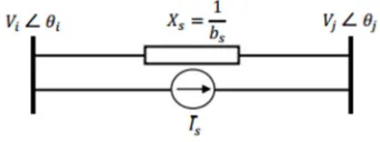
Converter 2 (inverter) is modeled as a serial voltage source inserted between two nodes i and j of a transmission network as shown in Figure 4.
Figure 4. Serial voltage converter representation.
VS : represents an ideal voltage source in series with XS, V a fictitious voltage. The resulting voltage diagram is shown in Figure 5.
Figure 5. Equivalent converter 2 voltage phasor diagram.
= (3) The voltage controllable in amplitude and phase, can be in the form:
= r (4)
where 0 < γ < 2π and 0 < r < rmax.
To obtain the UPFC injection model [15], this series voltage source is replaced by an equivalent current source in parallel with the line where (refer to Figure 6).
0 5 10 15 20 25 30 35 40
Noeud 0.75
0.8 0.85 0.9 0.95 1 1.05 1.1
Figure 6. Voltage source replaced by a current source.
The current corresponds to an injection of the powers ̅ and ̅ respectively at nodes i and j. At node i, the power injected by the series part of the UPFC is:
̅ = ̅ ∗ (5) So we have:
̅ = " ∗ (6) That means:
̅ " #sin ' " #cos ' (7)
Similarly, at node j, the power injected by the series part is:
̅ = ̅ ∗ (8) ̅ = " ∗ (9) By posing * * * then:
̅ " sin +* ', " cos * ' (10)
The injection model of the serial converter is therefore summarized by two loads as shown in Figure 7.
Figure 7. Injection model of the serial converter.
4.1.2. Injection model of the UPFC
As described above, the converter 1 provides the active power demanded by the converter 2. We therefore have -./01 -./01#.
The apparent power of the converter 2 in series with the line is: ./01# ̅∗ .
./01# " 13
451 6
7 (11)
Active power from converter 1 is therefore:
-./01 -./01# " sin+* * ', " #sin ' (12)
In addition, the converter 1 also makes it possible to supply or absorb reactive power. This reactive power is independently controlled by the UPFC and can therefore be
modeled by a separate reactive source which will be noted: 8./01 .
The injection model of the UPFC is thus obtained by adding the power equations derived from the model of the serial source (Figure 7) to the power -./01 8./01 (see Figure 8). The model can be added to the power flow equations by summing UPFC power injection equations at nodes i and j.
Figure 8. UPFC model.
4.2. Formulation of the Optimization Problem
4.2.1. Optimization Criteria
The resolution of this optimization problem consists in minimizing the following objective functions 9 , 9#, 9; and 9<.
Reduction of active losses
9 -=>?= @A? B= ∑ D EGF # (13)
With HI the number of branches in the network, D the resistence of the jth line and the current.
Voltage profil improving
9# JK ∑ LEGR M3NOPM3NOP5M3Q #
(14)
With S the voltage of the node i, S>=T the reference voltage at node i and HU sthe number of network nodes.
Installation cost reduction
The installation cost of the UPFC is proportional to its size in MVar. This cost is 40$/kVar [19].
So we have:
9; 40000 X YZTA (15)
With YZTA the operating range of the UPFC in MVar. Balancing of branches power transfer
9< ∑ L6[\]6 Q # EF
G (16)
With and ^@7 respectively the transited power and the maximum power of the jth branch.
4.2.2. Constraints of Optimization
Equality constraints
-_ -A X ∑ `
a bacos *a casin *a d 0 ER
aG (17)
8_ 8A X ∑ `
a basin *a cacos *a d 0 ER
aG (18)
With -_ and 8_ the active and reactive powers generated at node i, -A and 8A the load active and reactive powers at node i. b and c represent the conductance and susceptance of the branch between nodes i and j.
Inequality constraints
^ E e e ^@7 (19)
e ^@7 (20)
0 f " f "^@7 (21)
0 f ' f 2h (22) With ^ E the minimum voltage limit, equal to -10% of the ith node nominal voltage (according to CEB standards).
^@7 the maximum voltage limit, equal to + 10% of the
nominal value of the ith node. "^@7 0.1 p.u the maximum amplitude of the series voltage that can be injected by the UPFC.
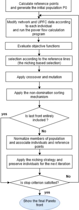
4.3. The Genetic Algorithm U-NSGA-III
Genetic algorithms are metaheuristic methods of optimization. They are inspired by the principle of biological evolution of living species. They are algorithms very well adapted to the treatment of multiobjective optimization problems [16]. There are several genetic algorithms among which we have: Nondominated Sorting Genetic Algorithm (NSGA), NSGA-II, NSGA-III and NSGA-III. The NSGA-III is developed in 2015 by Seada and Deb [17]. U-NSGA-III begins with a set of N randomly generated population individuals and a set of reference points. These reference points create reference lines that ensure diversity. At the tth generation, the entire population Pt is subjected to the following operations. First a selection of members who must participate in the reproduction is done through a selection operator named niching based selection. Based on this selection, an inherit population Qt is generated through
recombination and mutation operators. To ensure elitism, a selection of N individuals is made in the population Rt = Pt U
Qt in order to choose which members of the population will
survive for the next generation. For this, several operations are performed. First, the Rt population is subjected to
non-dominance sorting as in the case of NSGA-II described in [18]. This sorting consists in preserving one by one the non-dominance fronts in Pt+1 until all the solutions of a last front
named Fl cannot be included without exceeding the size N of
the population. To choose the rest of the individuals who must supplement the survivors of the next generation Pt+1, the
following steps are performed. At first, the members of Fl
and Pt+1 are normalized and then each associated with one of
the reference lines. Then, a strategy called Niching strategy is used to choose the members of Fl associated with the least
sought reference points. Once the N members of Pt+1 are
obtained, the process start again until the stopping criterion is
verified. The placement optimization of the UPFC by U-NSGA-III was carried out by adapting this algorithm. The flowchart in Figure 9 describes the optimal placement algorithm for an UPFC developed with U-NSGA-III.
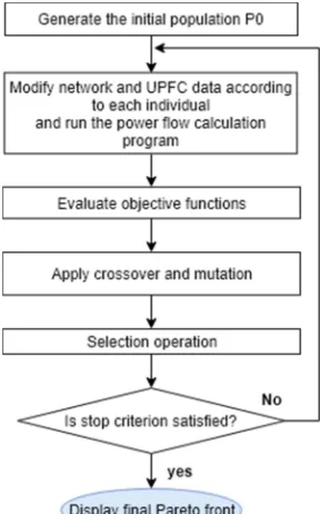
4.4. Differential Evolution Algorithm
Differential evolution (DE) is a population-based metaheuristic, introduced by Storn and Price in 1997. It is inspired by the principle of genetic algorithms (mutation and crossover operators) but remains a purely mathematical metaheuristic with geometric search strategies (simplex type). In our case, each individual of the population represents a configuration of the UPFC in the network.
Figure 9. Optimization flowchart of UPFC placement by U-NSGA-III.
Figure 10. Optimization flowchart of UPFC placement by DE.
4.5. Genotype of an Individual
The chromosome of an individual (potential solution) is shown in Figure 11.
Figure 11. Structure of a chromosome.
5. Results and Rentability Study
The placement optimization of an UPFC was carried out on the CEB's 42-node transmission network by specifying a population size of 750 for a generation number limited to 150 for the two algorithms. Figure 12 and Figure13 show the Pareto fronts obtained respectively by U-NSGA-III and DE.
Figure 12. Pareto Front of the U-NSGA-III.
Figure 13. Pareto Front of the DE.
To compare the performances of the two algorithms, the quality of the solutions of their respective Pareto fronts was evaluated using their respective hypervolume.
Table 2. Hypervolume calculation results.
U-NSGA-III DE
Hypervolume 159, 69. 10-4 117, 29. 10-4
This table shows that the value of the space dominated by the U-NSGA-III is greater than that of the DE. This shows that the Pareto front (solution set) obtained by the U-NSGA-III is better than that obtained by the DE.
The following Table 3 and 4 make it possible to compare the optimal solutions resulting respectively from the optimization by the two methods.
Table 3. Optimal solutions for each method.
Line Number Node Number r i jklmno
U-NSGA-III 3 6 0.099 282° 261 MVar
DE 3 6 0.089 265.36° 278, 42 MVar
Table 4. Phenotypes of optimal solutions.
Objectives function
pq pr ps pt
U-NSGA-III 32.65 MW 0, 06 $ 13126657.03 9.8
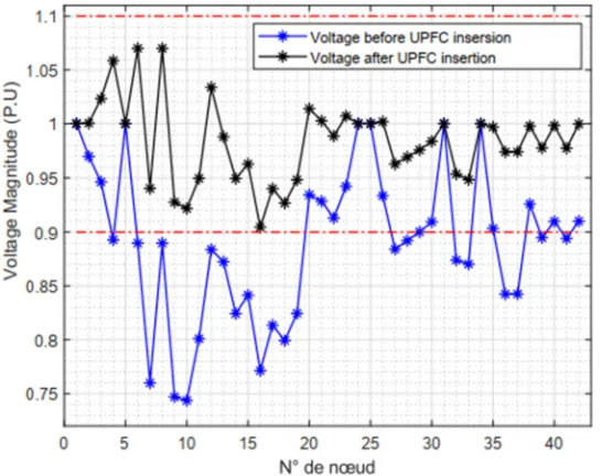
The following Figure 14 compares the voltage profile before and after positioning (in the 2025’s scenario studied).
Figure 14. Voltage profile after UPFC insertion.
Table 5 presents a summary of the voltage improvements after positioning the UPFC with the optimal values obtained by the U-NSGA-III.
Table 5. Voltage state before and after insertion.
Without UPFC With UPFC
Number of unstable nodes 23 0
Voltage deviation 0, 7 0, 06
Figure 15 shows the overload rates in the different branches of the studied network.
Figure 15. Overload rate of network branches.
Table 6. Branch power flow.
Sans UPFC Avec UPFC
Number of overloaded branches 2 0
Overload rate 20, 01 9, 8
Active losses in MW 50, 66 MW 32, 65 MW
The investment cost uv of the project is the sum of the installation cost uMwx. of the UPFC and the cost uyz of the studies.
uv uMwx. uyz (23)
The cost uyz of studies represents 2% of the installation cost.
uv 1.02 uMwx. (24) uMwx. = 13126657, 025 US $ = 7 875 994 215 FCFA
So the investment cost is uv= 8 033 514 099 •u•€. The
economic valuation of energy losses is done by applying an average energy supply tariff u^ to CEB customers.
Thus, saving money R_an recorded over a year is calculated by the formula:
D@E = Δ‚ƒ × u^ (25)
With Δ‚Z the energy saved over one year due to the loss
reduction observed.
Δ‚Z= „ - … †… zY
‡ (26)
Δ‚Z= - × Kˆ (27)
Δ‚Z= 50.66 − 32.65 × 8760 − 730
Δ‚Z= 144620300 ‹Œℎ
In the case of the CEB network, the average cost u^= 58 •u•€ /‹Œℎ. So, D@E= 8387977400 •u•€.
The payback period PRI is calculated taking into account the annual cost uyy of maintenance and operation which
represents a maximum of 10% of the cost of installation.
uyy = 0.1 uMwx. and then:
-D = .•
•\‘5.’’ (28)
In the case of the CEB's electricity grid, we have:
PRI = 12 months 20 days
It is observed that the UPFC is positioned for his serial part on line 3 and his shunt portion at node 6. The two branches that were initially overloaded in this 2025's scenario are decongested after the placement. Losses of 50.66MW rose to 32.65MW, a reduction of 35.55%. These technical performances achieved will help stabilize this 161 kV transmission network and reduce nuisance tripping that could be due to exceeding thermal limits. Optimization by U-NSGA-III resulted in almost the same result as optimization by DE. In fact, the positions are identical and the difference between the losses by the two methods is 5.25%, 14.28% for the voltage deviations and 1.01% for the overload rates. Also, observing hypervolume values from different fronts, and although the results obtained from simulation by the two methods are almost identical, it can be concluded that U-NSGA-III is more efficient and more efficient than DE for
the problem dealt with.
The Figure 14 shows the new voltage profile after the positioning in the 2025's scenario. It is observed that the profile is significantly improved and that the lowest voltage value which was 0.74 p.u has risen to 0.91 p.u. The estimated optimization cost is 13126657.025 US dollars. This cost is obviously less than the cost of building new plants and lines that would normally be built in this scenario to decongest the network. The profitability study showed that the return on investment is obtained after 12 months 20 days. It should also be noted that the use of UPFC to relieve the power transmission network has no impact on the ecosystem compared to the construction of new energy infrastructure.
6. Conclusion
This paper presents the CEB’s network optimization through four criteria (voltage deviation, active losses, installation cost, load rate) for the optimal choice and placement of an UPFC in a transmission network by U-NSGA-III and DE. From the results obtained, it is found that the optimal selection and sizing of an UPFC contributes to the improvement of the technical performance of the transmission networks and can make it possible to postpone the huge investments needed to decongest a transmission network and reduce the greenhouse gases emission by avoiding new plants construction. To this end, this project of optimal placement of a UPFC in the CEB’s transmission network could be of interest to the CEB authorities because the return on investment time is 12 months 20 days, testifying to its profitability. It can be concluded that the results obtained are convincing, effective and efficient, and that the GA-based U-NSGA-III is more precise in terms of results with respect to DE. This application based on genetic algorithms can help transmission system operators to optimize the operation of their network to enhance its stability and reliability.
7. Data Availability
Datasets related to this article can be found at https://data.mendeley.com/datasets/wwm9gyrrc5/draft?a=4db 9de20-7ff7-461f-822b-6af9e6adc67a ([20]).
References
[1] A. OLOULADE, MOUKENGUE IMANO, A. VIANOU, et R. BADAROU, «Contribution à l’étude de la répartition de puissance et à l’évaluation des pertes dans les réseaux de transport et de distribution de la communauté électrique du Benin et de la société béninoise d’énergie électrique (CEB-SBEE)», p. 87‑90, juill-2016.
[3] R. W. Chang, « Mixed-Integer Method for Optimal UPFC Placement based on Line Flow-Based Equations », p. 6. [4] T. Khurshaid, D. P. Walde, D. Kuanr, et A. Varshney,
«Sensitivity Based Analysis for Optimal Location of UPFC to Reduce Power Loss and Congestion in Deregulated Electricity Market», vol. 4, no 5, p. 5, 2014.
[5] J. P. Navani, M. Goyal, et S. Sapra, «Optimal Placement of TCSC and UPFC for Enhancement of Steady State Security in Power System», no 2, p. 8.
[6] S. Singh, «OPTIMAL LOCATION OF UPFC IN POWER SYSTEM USING SYSTEM LOSS SENSITIVITY INDEX», vol. 1, no 7, p. 6.
[7] I. Shah, N. Srivastava, et J. Sarda, «Optimal placement of multi-type facts controllers using real coded genetic algorithm», in 2016 International Conference on Electrical, Electronics, and Optimization Techniques (ICEEOT), Chennai, India, 2016, p. 482‑487.
[8] E. Ghahremani et I. Kamwa, «Optimal placement of multiple-type FACTS devices to maximize power system loadability using a generic graphical user interface», IEEE Transactions on Power Systems, vol. 28, no 2, p. 764‑778, mai 2013.
[9] A. Bhandakkar Atul et L. Mathew, «Optimal Placement of Unified Power Flow Controller and Hybrid Power Flow Controller Using Optimization Technique», 2018.
[10] I. Made Wartana, J. G. Singh, W. Ongsakul, K. Buayai, et S. Sreedharan, «Optimal placement of UPFC for maximizing system loadability and minimize active power losses by NSGA-II», in 2011 International Conference & Utility Exhibition on Power and Energy Systems: Issues and Prospects for Asia (ICUE), Pattaya, Thailand, 2011, p. 1‑8.
[11] M. M. M. El-arini et R. S. S. Ahmed, «OPTIMAL LOCATION OF FACTS DEVICES TO IMPROVE POWER
SYSTEMS PERFORMANCE», Journal of Electrical Engineering, p. 9.
[12] H. I. Shaheen, G. I. Rashed, et S. J. Cheng, «Optimal location and parameter setting of UPFC for enhancing power system security based on Differential Evolution algorithm», International Journal of Electrical Power & Energy Systems, vol. 33, no 1, p. 94‑105, janv. 2011.
[13] B. V. Kumar et N. V. Srikanth, «A hybrid approach for optimal location and capacity of UPFC to improve the dynamic stability of the power system», Applied Soft Computing, vol. 52, p. 974‑986, mars 2017.
[14] CEB, «Communauté Electrique du Bénin». [En ligne]. Disponible sur: www.cebnet.org. [Consulté le: 15-déc-2018]. [15] M. Noroozian, L. Angquist, M. Ghandhari, et G. Andersson,
«Use of UPFC for optimal power flow control», IEEE Transactions on Power Delivery, vol. 12, no 4, p. 1629‑1634,
oct. 1997.
[16] Y. Collette et P. Siarry, Optimisation multiobjectif. Paris: Eyrolles, 2002.
[17] H. Seada et K. Deb, «U-NSGA-III: A Unified Evolutionary Algorithm for Single, Multiple, and Many-Objective Optimization», p. 30.
[18] K. Deb, A. Pratap, S. Agarwal, et T. Meyarivan, «A fast and elitist multiobjective genetic algorithm: NSGA-II», IEEE Transactions on Evolutionary Computation, vol. 6, no 2, p. 182‑197, avr. 2002.
[19] B. M. Wilamowski et J. D. Irwin, Éd., Power electronics and motor drives, 2nd ed. Boca Raton, FL: CRC Press, 2011. [20] Oloulade, Arouna, Ceb 42-bus network data, URL: