DOI10.1186/2190-8567-2-13
R E S E A R C H Open Access
Multiscale analysis of slow-fast neuronal learning
models with noise
Mathieu Galtier·Gilles Wainrib
Received: 19 April 2012 / Accepted: 26 October 2012 / Published online: 22 November 2012 © 2012 M. Galtier, G. Wainrib; licensee Springer. This is an Open Access article distributed under the terms of the Creative Commons Attribution License (http://creativecommons.org/licenses/by/2.0), which permits unrestricted use, distribution, and reproduction in any medium, provided the original work is properly cited.
Abstract This paper deals with the application of temporal averaging methods to recurrent networks of noisy neurons undergoing a slow and unsupervised modifica-tion of their connectivity matrix called learning. Three time-scales arise for these models: (i) the fast neuronal dynamics, (ii) the intermediate external input to the sys-tem, and (iii) the slow learning mechanisms. Based on this time-scale separation, we apply an extension of the mathematical theory of stochastic averaging with pe-riodic forcing in order to derive a reduced deterministic model for the connectivity dynamics. We focus on a class of models where the activity is linear to understand the specificity of several learning rules (Hebbian, trace or anti-symmetric learning). In a weakly connected regime, we study the equilibrium connectivity which gathers the entire ‘knowledge’ of the network about the inputs. We develop an asymptotic method to approximate this equilibrium. We show that the symmetric part of the con-nectivity post-learning encodes the correlation structure of the inputs, whereas the anti-symmetric part corresponds to the cross correlation between the inputs and their time derivative. Moreover, the time-scales ratio appears as an important parameter revealing temporal correlations.
M. Galtier (
)NeuroMathComp Project Team, INRIA/ENS Paris, 23 avenue d’Italie, Paris, 75013, France e-mail:[email protected]
M. Galtier
School of Engineering and Science, Jacobs University Bremen gGmbH, College Ring 1, P.O. Box 750 561, Bremen, 28725, Germany
G. Wainrib
Laboratoire Analyse Géométrie et Applications, Université Paris 13, 99 avenue Jean-Baptiste Clément, Villetaneuse, Paris, France
Keywords slow-fast systems·stochastic differential equations·inhomogeneous Markov process·averaging·model reduction·recurrent networks·unsupervised learning·Hebbian learning·STDP
1 Introduction
Complex systems are made of a large number of interacting elements leading to non-trivial behaviors. They arise in various areas of research such as biology, social sci-ences, physics or communication networks. In particular in neuroscience, the nervous system is composed of billions of interconnected neurons interacting with their en-vironment. Two specific features of this class of complex systems are that (i) exter-nal inputs and (ii) interexter-nal sources of random fluctuations influence their dynamics. Their theoretical understanding is a great challenge and involves high-dimensional non-linear mathematical models integrating non-autonomous and stochastic pertur-bations.
Modeling these systems gives rise to many different scales both in space and in time. In particular, learning processes in the brain involve three time-scales: from neu-ronal activity (fast), external stimulation (intermediate) to synaptic plasticity (slow). Here, fast time-scale corresponds to a few milliseconds and slow time-scale to min-utes/hour, and intermediate time-scale generally ranges between fast and slow scales, although some stimuli may be faster than neuronal activity time-scale (e.g., submil-liseconds auditory signals [1]). The separation of these time-scales is an important and useful property in their study. Indeed, multiscale methods appear particularly relevant to handle and simplify such complex systems.
First, stochastic averaging principle [2,3] is a powerful tool to analyze the impact of noise on slow-fast dynamical systems. This method relies on approximating the fast dynamics by its quasi-stationary measure and averaging the slow evolution with respect to this measure. In the asymptotic regime of perfect time-scale separation, this leads to a slow reduced system whose analysis enables a better understanding of the original stochastic model.
Second, periodic averaging theory [4], which has been originally developed for celestial mechanics, is particularly relevant to study the effect of fast deterministic and periodic perturbations (external input) on dynamical systems. This method also leads to a reduced model where the external perturbation is time-averaged.
It seems appropriate to gather these two methods to address our case of a noisy and input-driven slow-fast dynamical system. This combined approach provides a novel way to understand the interactions between the three time-scales relevant in our models. More precisely, we will consider the following class of multiscale stochastic differential equations (SDEs), with1, 2>0 two small parameters
dv=11[F (v,w,u(2t ))]dt+√1
1dB(t ),
dw=G(v,w) dt, (1)
rep-resents the value of the external input at timet. Random perturbations are included in the form of a diffusion term, and(B(t ))is a standard Brownian motion.
We are interested in the double limit1→0 and2→0 to describe the evolution of the slow variablewin the asymptotic regime where both the variablevand the ex-ternal input are much faster thanw. This asymptotic regime corresponds to the study of a neuronal network in which both the external inputu and the neuronal activity voperate on a faster time-scale than the slow plasticity-driven evolution of synaptic weightsW. To account for the possible difference of time-scales betweenvand the input, we introduce the time-scale ratioμ=1/2∈ [0,∞]. In the interesting case whereμ∈(0,∞), one needs to understand the long-time behavior of the rescaled periodically forced SDE for anyw0fixed
dv=F (v,w0, μt ) dt+(v,w0) dB(t ).
Recently, in an important contribution [5], a precise understanding of the long-time behavior of such processes has been obtained using methods from partial differen-tial equations. In particular, conditions ensuring the existence of a periodic family of probability measures to which the law ofvconverges as time grows have been identi-fied, together with a sharp estimation of the speed of mixing. These results are at the heart of the extension of the classical stochastic averaging principle [2] to the case of periodically forced slow-fast SDEs [6]. As a result, we obtain a reduced equation describing the slow evolution of variablew in the form of an ordinary differential equation,
dw
dt = ¯G(w),
whereG¯ is constructed as an average of G with respect to a specific probability measure, as explained in Section2.
This paper first introduces the appropriate mathematical framework and then fo-cuses on applying these multiscale methods to learning neural networks.
The individual elements of these networks are neurons or populations of neurons. A common assumption at the basis of mathematical neuroscience [7] is to model their behavior by a stochastic differential equation which is made of four different contributions: (i) an intrinsic dynamics term, (ii) a communication term, (iii) a term for the external input, and (iv) a stochastic term for the intrinsic variability. Assuming that their activity is represented by the fast variable v∈Rn, the first equation of system (1) is a generic representation of a neural network (functionF corresponds to the first three terms contributing to the dynamics). In the literature, the level of non-linearity of the functionF ranges from a linear (or almost-linear) system to spiking neuron dynamics [8], yet the structure of the system is universal.
introduced in [9]. It says that if both neurons A and B are active at the same time, then the synapses from A to B and B to A should be strengthened proportionally to the product of the activity of A and B. There are many different variations of this correlation-based principle which can be found in [10,11]. Another recent, unsuper-vised, biologically motivated learning rule is the spike-timing-dependent plasticity (STDP) reviewed in [12]. It is similar to Hebbian learning except that it focuses on causation instead of correlation and that it occurs on a faster time-scale. Both of these types of rule correspond toGbeing quadratic inv.
Previous literature about dynamic learning networks is thick, yet we take a signif-icantly different approach to understand the problem. An historical focus was the un-derstanding of feedforward deterministic networks [13–15]. Another approach con-sisted in precomputing the connectivity of a recurrent network according to the prin-ciples underlying the Hebbian rule [16]. Actually, most of current research in the field is focused on STDP and is based on the precise times of the spikes, making them ex-plicit in computations [17–20]. Our approach is different from the others regarding at least one of the following points: (i) we consider recurrent networks, (ii) we study the evolution of the coupled system activity/connectivity, and (iii) we consider bounded dynamical systems for the activity without asking them to be spiking. Besides, our approach is a rigorous mathematical analysis in a field where most results rely heav-ily on heuristic arguments and numerical simulations. To our knowledge, this is the first time such models expressed in a slow-fast SDE formalism are analyzed using temporal averaging principles.
The purpose of this application is to understand what the network learns from the exposition to time-dependent inputs. In other words, we are interested in the evolution of the connectivity variable, which evolves on a slow time-scale, under the influence of the external input and some noise added on the fast variable. More precisely, we intend to explicitly compute the equilibrium connectivities of such systems. This fi-nal matrix corresponds to the knowledge the network has extracted from the inputs. Although the derivation of the results is mathematically tough for untrained readers, we have tried to extract widely understandable conclusions from our mathematical results and we believe this paper brings novel elements to the debate about the role and mechanisms of learning in large scale networks.
Although the averaging method is a generic principle, we have made significant assumptions to keep the analysis of the averaged system mathematically tractable. In particular, we will assume that the activity evolves according to a linear stochastic differential equation. This is not very realistic when modeling individual neurons, but it seems more reasonable to model populations of neurons; see Chapter 11 of [7].
2 Averaging principles: theory
In this section, we present multiscale theoretical results concerning stochastic aver-aging of periodically forced SDEs (Section2.3). These results combine ideas from singular perturbations, classical periodic averaging and stochastic averaging princi-ples. Therefore, we recall briefly, in Sections2.1and2.2, several basic features of these principles, providing several examples that are closely related to the applica-tion developed in Secapplica-tion3.
2.1 Periodic averaging principle
We present here an example of a slow-fast ordinary differential equation perturbed by a fast external periodic input. We have chosen this example since it readily illus-trates many ideas that will be developed in the following sections. In particular, this example shows how the ratio between the time-scale separation of the system and the time-scale of the input appears as a new crucial parameter.
Example 2.1 Consider the following linear time-inhomogeneous dynamical system with1, 2>0 two parameters:
dv dt =
1
1
−v+sin
t 2
,
dw dt = −w
+v2.
This system is particularly handy since one can solve analytically the first ordinary differential equation, that is,
v(t )= 1
1+μ2
sin
t 2
−μcos
t 2
+v0e−
t 1,
where we have introduced thetime-scales ratio
μ:=1 2
.
In this system, one can distinguish various asymptotic regimes when1and2 are small according to the asymptotic value ofμ:
• Regime 1: Slow inputμ=0:
First, if1→0 and2is fixed, thenv(t )is close to sin(2t ), and fromgeometric
singular perturbation theory[21,22] one can approximate the slow variablewby the solution of
dw
dt = −w+
sin
t 2
2
.
of
dw
dt = −w+
1 2, since2π1 02πsin(s)2ds=12.
• Regime 2: Fast inputμ= ∞:
If2→0 and1is fixed, then the classical averaging principle implies thatv is close to the solution of
dv dt = −
v 1
,
so thatw can be approximated by
dw
dt = −w+
v0e−t /1
2
,
and when 1→ 0, one does not recover the same asymptotic behavior as in Regime 1.
• Regime 3: Time-scales matching 0< μ <∞:
Now consider the intermediate case where1is asymptotically proportional to
2. In this case,vcan be approximated on the fast time-scalet /1by the periodic solutionv¯μ(t )=1+1μ2(sin(μt )−μcos(μt )) of dvdt = −v+sin(μt ). As a conse-quence,wwill be close to the solution of
dw
dt = −w+
1 2(1+μ2), since2π1 02πv¯μ(t /μ)2dt=2(1+1μ2).
Thus, we have seen in this example that
1. the two limits1→0 and2→0 do not commute,
2. the ratioμbetween the internal time-scale separation1and the input time-scale
2is a key parameter in the study of slow-fast systems subject to a time-dependent perturbation.
2.2 Stochastic averaging principle
Time-scales separation is a key property to investigate the dynamical behavior of non-linear multiscale systems, with techniques ranging from averaging principles to geometric singular perturbation theory. This property appears to be also crucial to understanding the impact of noise. Instead of carrying a small noise analysis, a mul-tiscale approach based on thestochastic averaging principle[2] can be a powerful tool to unravel subtle interplays between noise properties and non-linearities. More precisely, consider a system of SDEs inRp+q:
dvt =1
F
vt,wtdt+√1
vt,wt·dB(t ),
with initial conditions v(0)=v0,w(0)=w0, and where w ∈Rq is called the slow variable,v∈Rp is the fast variable, withF,G,smooth functions ensuring the existence and uniqueness for the solution(v,w), and B(t ) ap-dimensional standard Brownian motion, defined on a filtered probability space(,F,P). Time-scale separation in encoded in the small parameter, which denotes in this section a single positive real number.
In order to approximate the behavior of(v,w)for small, the idea is to average out the equation for the slow variable with respect to the stationary distribution of the fast one. More precisely, one first assumes that for eachw∈Rqfixed, thefrozenfast SDE,
dvt=F (vt,w) dt+(vt,w)·dB(t ),
admits a unique invariant measure, denotedρw(dv). Then, one defines the averaged drift vector fieldG¯
¯
G(w):=
Rm
G(v,w)ρw(dv) (2)
andwthe solution of ddtw = ¯G(w)with the initial conditionw(0)=y0. Under some dissipativity assumptions, the stochastic averaging principle [2] states:
Theorem 2.1 For anyδ >0andT >0, lim
→0P t∈[sup0,T]
wt −wt2> δ
=0. (3)
As a consequence, analyzing the behavior of the deterministic solutionwcan help to understand useful features of the stochastic process(v,w).
Example 2.2 In this example we consider a similar system as in Example 2.1, but with a noise term instead of the periodic perturbation. Namely, we consider(v,w)
the solution of the system of SDEs,
dv= −1 v
dt+√σ
dB(t ),
dw=−w+v2dt,
with >0 a small parameter andσ >0 a positive constant. From Theorem2.1, the stochastic slow variablewcan be approximated in the sense of (3) by the determin-istic solutionwof
dw dt =
v∈R
−w+v2ρ(dv),
whereρ(dv)is the stationary measure of the linear diffusion process,
that is,
ρ(dv)= 1 σ√πe
−v2 σ2.
Consequently,wcan be approximated in the limit→0 by the solution of
dw
dt = −w+ σ2
2 .
Applying (3) leads to the following result: for anyT >0 andδ >0,
lim →0P
sup t∈[0,T]
wt−
y0−
σ2
2
e−t+σ
2 2
2> δ
=0.
Interestingly, the asymptotic behavior ofwfor smallis characterized by a deter-ministic trajectory that depends on the strengthσ of the noise applied to the system. Thus, the stochastic averaging principle appears particularly interesting when unrav-eling the impact of noise strength on slow-fast systems.
Many other results have been developed since, extending the set-up to the case where the slow variable has a diffusion component or to infinite-dimensional settings for instance, and also refining the convergence study, providinghomogenization re-sults concerning the limit of−1/2(w−w)or establishing large deviation principles (see [23] for a recent monograph). However, fewer results are available in the case of non-homogeneous SDEs, that is, when the system is perturbed by an external time-dependent signal. This setting is of particular interest in the framework of stochastic learning models, and we present the main relevant mathematical results in the follow-ing section.
2.3 Double averaging principle
Combining ideas of periodic and stochastic averaging introduced previously, we present here theoretical results concerning multiscale SDEs driven by an external time-periodic input. Consider(v,w)the solution of
dv= 1
1
F
v,w, t 2
dt+√1 1
v,w·dB(t ), dw=Gv,wdt,
(4)
witht→F (v,w, t )∈Rpaτ-periodic function and=(1, 2)∈R2+. Parameter1 represents the internal time-scale separation and2the input time-scale. We consider the case where both1and2are small, that is, a strong time-scale separation between the fast variablev∈Rp and the slow onew∈Rq, and a fast periodic modulation of the fast driftF (v,w,·).
Definition 2.1 We define the asymptotic time-scale ratio
μ:= lim
||→0
1
2
. (5)
Accordingly, we denote limμ||→0 the distinguished limit when 1→0, 2→0 with1/2→μ.
The following assumption is made to ensure existence and uniqueness of a strong solution to system (4). In the following,z1,z2will denote the usual scalar product for vectors.
Assumption 2.1 Existence and uniqueness of a strong solution
(i) The functionsF,G, andare locally Lipschitz continuous in the space vari-ablez. More precisely, for anyR >0, there exists a constantαR such that
F (z)−Fz≤αRz−z for anyz,z∈Rp+qwithz ≤Randz ≤R.
(ii) There exists a constantR >0 such that sup
z>R,t >0
(F (z, t ), G(z)),z
z2 <0.
To control the asymptotic behavior of the fast variable, one further assumes the following.
Assumption 2.2 Asymptotic behavior of the fast process: (i) The diffusion matrixis bounded
∃M>0 s.t.∀z,(z)< M
and uniformly non-degenerate
∃η0>0 s.t.∀v,z
(z)·(z)v,v≥η0v2. (ii) There existsr0<0 such that for allt≥0 and for allz,x∈Rp+q,
∇zF (z, t )·x,x≤r0x2.
According to the value ofμ∈ {0,R∗+,∞}, the stochastic averaging principle is based on a description of the asymptotic behavior of various rescaled fast frozen processes. More precisely, under Assumptions2.1and2.2, one can deduce that:
• For any fixedw0∈Rqandt0>0 fixed, the law of the rescaled time-homogeneous frozen process,
dv=F (v,w0, t0) dt+(v,w0) dB(t ),
converges exponentially fast to a unique invariant probability measure denoted by
• For any fixedw0∈Rq, there exists a μτ-periodic evolution system of measures
νw0
μ (t, dv), different fromρw0,t(dv)above, such that the law of the rescaled time-inhomogeneous frozen process,
dv=F (v,w0, μt ) dt+(v,w0) dB(t ), (6) converges exponentially fast towardsνw0
μ (t,·), uniformly with respect tow0 (cf. theAppendixTheoremA.1).
• For any fixedw0∈Rq, the law of the rescaled time-homogeneous frozen process,
dv= ¯F (v,w0) dt+(v,w0) dB(t ),
whereF (¯ v,w0):=τ−10τF (v,w0, t ) dt, converges exponentially fast towards a unique invariant probability measure denoted byρ¯w0(dv).
According to the value ofμ, we introduce a vector fieldG¯μwhich will play a role similar toG¯ introduced in equation (2).
Definition 2.2 We defineG¯μ:Rq→Rqas follows. In the time-scale matching case, that is, when 0< μ <∞, then
¯
Gμ(w):=
τ μ
−1 τ
μ
0
v∈Rp
G(v,w)νμw(t, dv) dt. (7)
Notation We may denote the periodic system of measuresνwμ(t, dv)associated with (6) byνμw[F,](t, dv)to emphasize its relationship withF and. Accordingly, we may denoteG¯μ(w)byG¯[μF,](w).
We are now able to present our main mathematical result. Extending Theorem2.1, the following theorem describes the asymptotic behavior of the slow variable w when→0 with1/2→μ. We refer to [6] for more details about the full mathe-matical proof of this result.
Theorem 2.2 Letμ∈(0,∞).Ifwis the solution of
dw
dt = ¯Gμ(w) withw(0)=w
(0), (8)
then the following convergence result holds,for allT >0andδ >0: μ
lim
||→0P t∈[sup0,T]
w
t −wt 2
> δ
=0.
Remark 2.1
• Slow input: If one considers the case where the limit1→0 is takenfirst, so that from Theorem2.1with fast variablev and slow variablesw andt (with the trivial equationt˙=1),wis close in probability on finite time-intervals to the solution of the following inhomogeneous ordinary differential equation:
dw˜
dt =
v∈Rp
G(v,w˜)ρw˜,t /2(dv):= ˜G(w˜, t / 2).
Then taking the limit2→0, one can apply the deterministic averaging prin-ciple to the fast periodic vector field G(˜ w, t /2), so thatw˜ converges when
2→0 to the solution of
dw
dt =τ
−1
τ
0
˜
G(v,w) dt= ¯G0(w), where
¯
G0(w):=τ−1
τ
0
v∈Rp
G(v,w)ρw,t(dv) dt.
• Fast input: If the limit2→0 is taken first, one first has to perform a classical averaging of the periodic driftF (v,w, t /2)leading to the homogeneous system of SDEs (4), but withF (¯ v,w)instead ofF (v,w, t /2). Then, an application of Theorem2.1on this system gives an averaged vector field
¯
G∞(w):=
v∈Rp
G(v,w)ρ¯w(dv).
2. To study the extremal casesμ=0 andμ= ∞in full generality, one would need to consider all the possible relationships between 1 and2, not only the linear one as in the present article, but also of the type1=2αfor example. In this case, we believe that the regimeα <1 converges to the same limit as taking the limit2 first and the regimeα >1 corresponds to taking the limit1first. The intermediate regimeα=1 seems to be the only one for which the limit cannot be obtained by combining classical averaging principles. Therefore, the present article is focused on this case, in which the averaged system depends explicitly on the scaling pa-rameterμ. Moreover, in terms of applications, this parameter can have a relatively easy interpretation in terms of the ratio of time-scales between intrinsic neuronal activity and typical stimulus time-scales in a given situation. Although the zeroth order limit (i.e., the averaged system) seems to depend only on the position ofα
with respect to 1, it seems reasonable to expect that the fluctuations around the limit would depend on the precise value of α. This is a difficult question which may deserve further analysis.
The case 0< μ <∞is already very rich in the sense that it combines simul-taneously both the periodic and stochastic averaging principles in a new way that cannot be recovered by sequential applications of those principles. A particular role is played by the frozen periodically-forced SDE (6). The equivalent of the quasi-stationary measure ρw of Theorem2.1is given by the asymptotically pe-riodic behavior of equation (6), represented by the pepe-riodic family of measures
3. By a rescaling of the frozen process (6), one deduces the followingscaling rela-tionships:
νμw[F,](t, dv)=ν1w
F μ,
√μ
(μt, dv)
and
¯
G[μF,](w)= ¯G[ F μ,
√μ]
1 (w).
Therefore, if one knows, in the caseμ=1, the averaged vector field associated with the fast process generated by a driftF and a diffusion coefficientσ, denoted
¯
G1[F,], it is possible to deduceG¯μin the general caseμ∈(0,∞)with a change
F →μFand→ √μ.
4. It seems reasonable to expect that the above result is still valid when considering ergodic, but not necessarily periodic, time dependency of the functionF (v,w,·). In equation (7), instead of integrating νμw(t, dv)over one period, one should in-tegrate it with respect to an ergodic stationary measure. However, this extension requires non-trivial technical improvements of [5] which are beyond the scope of this paper.
2.3.1 Case of a fast linear SDE with periodic input
We present here an elementary case where one can compute explicitly the quasi-stationary time-periodic family of measuresνwμ(t, x), when the equation for the fast variable is linear. Namely, we considerv∈Rpthe solution of
dv(t )=−A·v(t )+u(μt )dt+·dB(t ),
with initial conditionv(0)=v0∈Rp, and whereA∈Rp×pis a matrix whose eigen-values have positive real parts andu(·)is aτ-periodic function.
We are interested in the large time behavior of the law ofv(t ), which is a time-inhomogeneous Ornstein-Uhlenbeck process. From [5] we know that its law con-verges to aτ-periodic family of probability measuresν(t, dv). Due to the linearity in the previous equation,ν(t, dv)is Gaussian with a time-dependent mean and a con-stant covariance matrix
ν(t, dv)=Nv¯(t ),Q(dv),
wherev¯is the μτ-periodic attractor ofddtv¯= −A· ¯v(t )+u(μt ),i.e.,
¯
v(t )=
t
−∞e
−A(t−s)u(μs) ds,
andQis the unique solution of the Lyapunov equation
Indeed, if one denotesc(t )=v(t )− ¯v(t ), thenc(t )is a solution of the classical ho-mogeneous Ornstein-Uhlenbeck equation
dc(t )= −Ac(t ) dt+dB(t ),
whose stationary distribution is known to be a centered Gaussian measure with the covariance matrixQsolution of (9); see Chapter 3.2 of [24]. Notice that ifAis self-adjoint with respect to(·)−1(i.e.,A·(·)=(·)·A), then the solution isQ=A−1·(2·)=(·2)·A−1, which will be used in AppendixB.2.
Hence, in the linear case, the averaged vector field of equation (7) becomes
¯
Gμ(w):=
τ μ
−1 τ
μ
0
v∈Rp
Gv¯(t )+v,wN0,Q(dv) dt, (10)
whereNx,Qis the probability density function of the Gaussian law with meanx∈Rq
and covarianceQ∈Rp×p.
Therefore, due to the linearity of the fast SDE, the periodic system of measureν
is just a constant Gaussian distribution shifted by a periodic function of timev(t ). In caseGis quadratic inv, this remark implies that one can perform independently the integral over time and overRpin formula (10) (noting that the crossed term has a zero average). In this case, contributions from the periodic input and from noise appear in the averaged vector field in an additive way.
Example 2.3 In this last example, we consider a combination between Example2.1 and Example2.2, namely we consider the following system of periodically forced SDEs:
dv= 1 1
−v+sin
t 2
dt+√σ 1
dB(t ),
dw=−w+v2dt.
As in Example2.1and as shown above, the behavior of this system when both1 and2are small depends on the parameterμdefined in (5). More precisely, we have the following three regimes:
• Regime 1: slow input:
¯
G0(w)= −w+
σ2
2 + 1 2.
• Regime 2: fast input:
¯
G∞(w)= −w+σ
2 2 .
• Regime 3: time-scale matching:
¯
Gμ(w)= −w+
σ2
2.4 Truncation and asymptotic well-posedness
In some cases, Assumptions2.1-2.2may not be satisfied on the entire phase space
Rp×Rq, but only on a subset. Such situations will appear in Section3when consid-ering learning models. We introduce here a more refined set of assumptions ensuring that Theorem2.2still applies.
Let us start with an example, namely the following bi-dimensional system with white noise input:
dv=1(−lv+wv) dt+√σ
dB(t ),
dw=(−κw+(v)2) dt, (11)
with >0,σ >0,l >0,μ >0.
For the fast drift−(l−w)vto be non-explosive, it is necessary to havew < l−α
withα >0 for all time. The concern about this system comes from the fact that the slow variablewmay reachldue to the fluctuations captured in the termv2, for instance, ifκ is not large enough. Such a system may have exponentially growing trajectories. However, we claim that for small enough,wwill remain close to its averaged limitw for a very long time, and if this limit remains belowl−α, then
w can be considered as well-posed in the asymptotic limit →0. To make this argument more rigorous, we suggest the following definition.
Definition 2.3 A stochastic differential equation with a given initial condition is asymptotically well posed in probability if for the given initial condition,
1. a unique solution exists until a random timeτ 2. for allT >0,
lim
→0P[τ≥T] =1.
We give in the following proposition sufficient conditions for system (4) to be asymp-totically well posed in probability and to satisfy conclusions of Theorem2.2.
Let us introduce the following set of additional assumptions. Assumption 2.3 Moment conditions:
(i) There existsp >2 such that for anyT >0, sup
E sup 0≤t≤T
v t
p
+wt p
<∞.
(ii) For anyT >0 and any bounded subsetKofRq, sup
1>0,2>0,w∈K
E sup 0≤t≤T
Gvt,w 2
<∞.
moments ofv; therefore, the moment conditions (i) and (ii) will be satisfied without any difficulty. Moreover, if one considers non-linear models for the variablev, then the Gaussian property may be lost; however, adding sigmoidal non-linearity has, in general, the effect of bounding the dynamics, thus making these moment assumptions reasonable to check in most models of interest.
Property 2.3 If there exists a subsetE ofRqsuch that
1. The functionsF,G,satisfy Assumptions2.1-2.3restricted onRp×E. 2. Eis invariant under the flow ofG¯μ,as defined in(7).
Then for any initial condition w0∈E, system (4) is asymptotically well posed in probability andw satisfies the conclusion of Theorem2.2.
Proof See AppendixA.2.
Here, we show that it applies to system (11). First, withEα= {w∈R, w < l−α}, for someα∈ ]0, l[, it is possible to show that Assumptions 2.1-2.2are satisfied on
Rp×E
α. Then, as a special case of (10), we obtain the following averaged system:
dw
dt = −κw+ σ2
2(l−w):= ¯G(w).
It remains to check that the solution of this system satisfies
∃α >0, such thatw(0) < l−α ⇒ ∀t >0, w(t ) < l−α,
that is, the subsetEα is invariant under the flow ofG¯. This property is satisfied as soon as
η:=2σ
2
κl2 <1.
Indeed, one can show thatG(w)¯ =0 admits two solutions iffη <1,
w±= l
2(1±
1−η)∈(0, l),
and thatw− is stable whereasw+ is unstable. Thus, ifw(0) < l−αwithα=l− w+>0, thenw(t ) < l−αfor allt >0. In fact, the invariance property is true for all
α∈ ]l−w−, l−w+[.
3 Averaging learning neural networks
difficult and we only manage to get explicit results for simple systems where the fast activity dynamics is linear. In the three last subsections, we push the analysis for three examples of increasing complexity.
In the following, we always consider that the initial connectivity is 0. This is an arbitrary choice but without consequences, because we focus on the regime where there is a single globally stable equilibrium point (see Section3.2.3).
3.1 A generic learning neural network
We now introduce a large class of stochastic neuronal networks with learning models. They are defined as coupled systems describing the simultaneous evolution of the activity ofn∈Nneurons and the connectivity between them. We definev∈Rn, the
activity fieldof the network, andW∈Rn×n, theconnectivity matrix. Each neuron variableviis assumed to follow the SDE
dvi=fi(vi)+ui
dt+·dBi(t ),
where the function fi characterizes the intrinsic non-linear dynamical behavior of neuroniandui is the input received by neuroni. The stochastic term·dBi(t )is added to account for internal sources of noise. In terms of notations,(B(t ))t≥0 is a standardn-dimensional Brownian motion,is ann×nmatrix, possibly function of vor other variables, and·dBi(t )denotes theith component of the vector·dB(t ). The inputui to neuronihas mainly two components: the external inputuexti and the input coming from other neurons in the network usyni . The latter is a prioria complex combination of post-synaptic potentials coming from many other neurons. The coefficientWij of the connectivity matrix accounts for the strength of a synapse
j→i. Note that neurons can be connected to themselves,i.e.,Wiiis not necessarily null. Thus, we can write
usyni :=S
n
j=1
WijH(vi,vj)
,
whereS:R→RandHis a function taking the history ofvi andvj and returning a real for each timet (to take convolutions into account). In practical cases, they are often taken to be sigmoidal functions. We abusively redefineSandHas vector valued operators corresponding to the element-wise application of their real counterparts. We also define the functionF:Rn→Rnsuch thatF(v)i=fi(vi). Together with a slow generic learning rule, this leads to defining astochastic learning modelas the following system of SDEs.
Definition 3.1
dv=1[F(v)+S(W·H(v))+uext(t )]dt+√1
(v
,W)·dB(t ),
Before applying the general theory of Section2, let us make several comments about this generic model of neural network with learning. This model is a non-autonomous, stochastic, non-linear slow-fast system.
In order to apply Theorem2.2, one needs Assumptions2.1,2.2, and2.3to be sat-isfied, restricting the space of possible functionsS,H,F,, andG. In particular, Assumption2.2(ii) seems rather restrictive since it excludes systems with multiple equilibria and suggests that the general theory is more suited to deal with rate-based networks. However, one should keep in mind that these assumptions are only suffi-cient, and that the double averaging principle may work as well in systems which do not satisfy readily those assumptions.
As we will show in Section3.3, a particular form of history-dependence can be taken into account, to a certain extent. Indeed, for instance, if the functionF is ac-tually a functional of the past trajectory of variablevwhich can be expressed as the solution of an additional SDE, then it may be possible to include a certain form of history-dependence. However, purely time-delayed systems do not enter the scope of this theory, although it might be possible to derive an analogous averaging method in this framework.
The noise term can be purely additive or set by a particular function(v,W)
as long as it satisfies Assumption2.2(i), meaning that it must be uniformly non-degenerate.
In the following subsection, we apply the averaging theory to various combina-tions of neuronal network models, embodied by choices of funccombina-tionsS, H, F,, and various learning rules, embodied by a choice of the functionG. We will also analyze the obtained averaged system, describing the slow dynamics of the connec-tivity matrix in the limit of perfect time-scale separation and, in particular, study the convergence of this averaged system to an equilibrium point.
3.2 Symmetric Hebbian learning
One of the simplest, yet non-trivial, stochastic learning models is obtained when con-sidering
• A linear model for neuronal activity, namelyfi(vi)= −lvi withla positive con-stant.
• A linear model for the synaptic transmission, namelyS(vi)=vi andH(vi,vj)=
vj.
• A constant diffusion matrix (additive noise) proportional to the identity=
σ I d(spatially uncorrelated noise).
• A Hebbian learning rule with linear decay, namelyGij(W,v)= −κWij+vivj. Actually, it corresponds to the tensor product:{v⊗v}ij=vivj.
This model can be written as follows:
dv=11(−L·v+W·v+u(2t )) dt+√σ1dB(t ),
dW
dt =G(v
,W)= −κW+v⊗v, (12) where neurons are assumed to have the same decay constant:L=lId;uis a peri-odic continuous input (it replacesuextin the previous section);σ, 1, 2, κ∈R+with
The first question that arises is about the well-posedness of the system: What is the definition interval of the solutions of system (12)? Do they explode in finite time? At first sight, it seems there may be a runaway of the solution if the largest real part among the eigenvalues ofWgrows bigger thanl. In fact, it turns out this scenario can be avoided if the following assumption linking the parameters of the system is satisfied.
Assumption 3.1 There existsp∈ ]0,1[such that
σ2l
2p(1−p)+ u2m p(1−p)2
< κl3,
whereum=supt∈R+u(t )2.
It corresponds to making sure the external (i.e.,um) or internal (i.e.,σ) excitations are not too large compared to the decay mechanism (represented byκandl). Note that ifp∈ ]0,1[,umandd are fixed, it is sufficient to increaseκ orlfor this assumption to be satisfied.
Under this assumption, the space
Ep=
W∈Rn×n:Wis symmetric,W≥0 andW< pL
is invariant by the flow of the averaged systemG¯, whereW≥0 meansWis semi-definite positive andW< pL means pL−Wis definite positive. Therefore, the averaged system is defined and bounded onR+. The slow/fast system being asymp-totically close to the averaged system, it is therefore asympasymp-totically well-defined in probability. This is summarized in the following theorem.
Theorem 3.1 If Assumption3.1is verified forp∈ ]0,1[,then system(12)is asymp-totically well posed in probability and the connectivity matrix W,the solution of system(12),converges toWin the sense that for allδ, T >0,
μ lim
→0P t∈[sup0,T]
Wt −Wt2> δ
=0,
whereWis the deterministic solution of
dWij
dt = ¯G(W)ij= − κWij decay
+μ
τ
τ
μ
0
¯
vi(s)vj¯ (s) ds
correlation
+σ2
2 (L−W)
−1 ij
noise
, (13)
wherev¯(t )is theμτ-periodic attractor ofddtv¯=(W−L)· ¯v+u(μt ),whereW∈Rn×n
is supposed to be fixed.
3.2.1 Noise term
As seen in Section 2, in the linear case, the noise term Q is the unique solution of the Lyapunov equation (9) withA=W−Land=σ I d. Because the noise is spatially uncorrelated and identical for each neuron and also because the connectivity is symmetric, observe thatQ=σ22(L−W)−1is the unique solution of the system.
In more complicated cases, the computation of this term appears to be much more difficult as we will see in Section3.4.
3.2.2 Correlation term
This term corresponds to the auto-correlation of neuronal activity. It is only implicitly defined; thus, this section is devoted to finding an explicit form depending only on the parametersl,μ,τ, the connectivityW, and the inputsu. Actually, one can perform an expansion of this term with respect to a small parameter corresponding to aweakly connected expansion. Most terms vanish if the connectivityWis small compared to the strength of the intrinsic decaying dynamics of neuronsl.
The auto-correlation term of aμτ-periodic function can be rewritten as
¯
v· ¯vij=
τ
μ
0 ¯
vi(s)vj¯ (s) ds.
With this notation, it is simple to think ofvas a ‘semi-continuous matrix’ ofRn×[0,μτ[.
Hence, the operator ‘·’ can be though of as a matrix multiplication. Similarly, the transpose operator turns a matrixv¯∈Rn×[0,μτ[into a matrixv¯∈R[0,
τ
μ[×n. See
Ap-pendixB.1for details about the notations.
It is common knowledge, see [17] for instance, that this term gathers information about the correlation of the inputs. Indeed, if we assume that the input is sufficiently slow, thenv¯ has enough time to converge tou(t )for allt∈ [0,+∞[. Therefore, in the first orderv¯(t )(W−L)−1·u(t ). This leads tov¯· ¯v(W−L)−1·u·u·(W− L)−1. In the weakly connected regime, one can assume thatW−L −Lleading to
¯
v· ¯vl12u·uwhich is the auto-correlation of the inputs.
Actually, without the assumption of a slow input, lagged correlations of the in-put appear in the averaged system. Before giving the expression of these temporal correlations, we need to introduce some notations. First, define the convolution filter
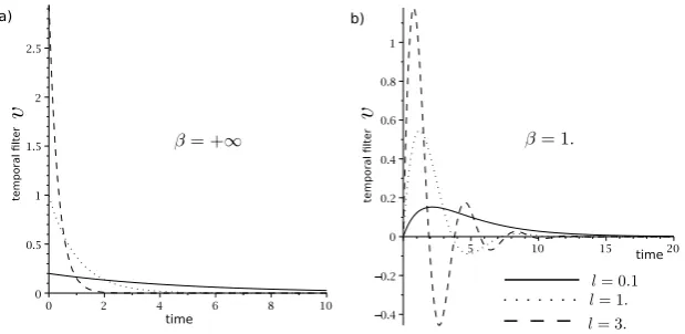
gl/μ:t → μle−
l
μtH (t ), where H is the Heaviside function. This family of
func-tions is displayed for different values ofμl in Figure4(a). Note thatgl/μ→δ0when l
μ→ +∞, whereδ0is the Dirac distribution centered at the origin. In this asymptotic regime, the convolution filter and its iteratesgl/μ∗ · · · ∗gl/μare equal to the identity.
We also define the filtered correlation of the inputsCk,p∈Rn×nby Ck,qdef= 1
u2 mτ
u∗gl/μ(k+1)·u∗gl/μ(q+1),
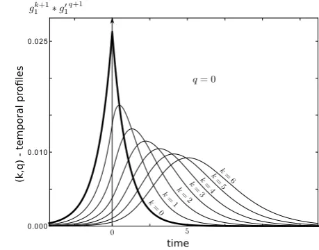
Fig. 1 This shows the (k, q)-temporal profiles with
l
μ=1,i.e., the functions
g(k1+1)∗g1(q+1)forq=0 and kranging from 0 to 6. For k=q=0, the temporal profile is even and this also occurs to be true for anyk=q. Whenk > q, the function reaches its maximum for strictly positive values that grow with the differencek−q. Besides, the temporal profiles are flattened whenk+qincreases.
functions. It is easy to show that this is similar to computing the cross-correlation of the inputs with the inputs filtered by another function,
Ck,q= 1
u2 mτ
u∗g(kl/μ+1)∗gl/μ(q+1)·u
= 1
u2 mτ
u·u∗g(kl/μ+1)∗gl/μ(q+1), (14)
which motivates the definition of the(k, p)-temporal profileg(kl/μ+1)∗gl/μ(q+1), where
(gl/μ )(k)(t )=(gl/μ(k))(t )=gl/μ(k)(−t ). This notation is deliberately similar to that of the transpose operator we use in the proofs. These functions are shown in Figure1. We have not found a way to make them explicit; therefore, the following remarks are simply based on numerical illustrations. Whenk=q, the temporal profiles are centered. The larger the differencek−q, the larger the center of the bell. The larger the sumk+q, the larger the standard deviation. This motivates the idea thatCk,p can be thought of as thek−qlagged correlation of the inputs. One can also say that C10,10is more blurred thanC0,0in the sense that the inputs are temporally integrated over a ‘wider’ window in the first case.
Observe thatgl/μ(k+1)(t )= lk+1
μk+1k!tke−
l
μtH (t ). Therefore,g(k+1)
l/μ 1= (k+1)
k! =1. Thanks to Young’s inequality for convolutions, which says that u∗g(k)l/μ2 ≤
u2g(k)l/μ1, it can be proved thatCk,q2≤1.
We intend to express the correlation term as an infinite converging sum involving these filtered correlations. In this perspective, we use a result we have proved in [25] to write the solution of a general class of non-autonomous linear systems (e.g.,
dv¯
Lemma 3.2 Ifv¯is the solution,with zero as initial condition,of ddtv¯ =(W−L)· ¯v+ u(t )it can be written by the sum below which converges ifWis inEpforp∈ ]0,1[.
¯
v=
+∞
k=0 Wk
lk+1·u∗g (k+1) l ,
wheregl:t→le−ltH (t ).
Proof See LemmaB.2in AppendixB.2. This is a decomposition of the solution of a linear differential system on the basis of operators where the spatial and temporal parts are decoupled. This important step in a detailed study of the averaged equation cannot be achieved easily in models with non-linear activity. Everything is now set up to introduce the explicit expansion of the correlation we are using in what follows. Indeed, we use the previous result to rewrite the correlation term as follows.
Property 3.3 The correlation term can be written
μ τv¯· ¯v
=u2m
l2
+∞
k,q=0 Wk
lk ·C k,q·W
q
lq .
Proof See TheoremB.3in AppendixB.2. This infinite sum of convolved filters is reminiscent of a property of Hawkes pro-cesses that have a linear input-output gain [26].
The speed of inputs characterized byμonly appears in the temporal profilesg(k)l/μ∗ gl/μ (q). In particular, if the inputs are much slower than neuronal activity time-scale,
i.e.,μ=0, theng+∞=δ0andu∗g+∞=u. Therefore,Ck,q=C0,0and the sums in the formula of Property3.3are separable, leading tov¯· ¯v=(L−W)−1·u·u·(L− W)−1, which corresponds to the heuristic result previously explained.
Therefore, the averaged equation can be explicitly rewritten
dW
dt = ¯G(W)= −κW+ u2m
l2
+∞
k,q=0 Wk
lk ·C k,q·W
q
lq +
σ2
2 (L−W)
−1. (15)
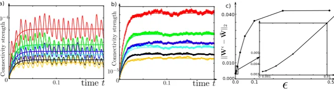
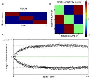
In Figure2, we illustrate this result by comparing, for different=1=2(i.e., we chooseμ=1 in this example), the stochastic system and its averaged version. The above decomposition has been used as the basis for numerical computation of trajectories of the averaged system.
3.2.3 Global stability of the equilibrium point
Fig. 2 The first two figures, (a) and (b), represent the evolution of the connectivity for original stochastic system (12), superimposed with averaged system (13), for two different values of: respectively=0.01 and=0.001, where we have chosen=1=2. Each color corresponds to the weight of an edge in
a network made ofn=3 neurons. As expected, it seems that the smaller, the better the approximation. This can be seen in the picture (c) where we have plotted the precision on they-axis andon thex-axis. The parameters used here arel=12,μ=1,κ=100,σ=0.05. The inputs have a random (but frozen) spatial structure and evolve according to a sinusoidal function.
is kept smaller than 3l,i.e., Assumption3.1is verified withp≤ 13, then the dynam-ics is trivial: the system converges to a single equilibrium point. Indeed, under the previous assumption, the system can be writtenG(¯ W)= −κW+F (W), whereF is a contraction operator onE1
3. Therefore, one can prove the uniqueness of the fixed point with the Banach fixed point argument and exhibit an energy function for the system.
Theorem 3.4 If Assumption3.1is verified forp≤ 13,then there is a unique equilib-rium point in the invariant subsetEpwhich is globally,asymptotically stable.
Proof See TheoremB.4in AppendixB.2. The fact that the equilibrium point is unique means that the ‘knowledge’ of the net-work about its environment (corresponding by hypothesis to the connectivity) even-tually is unique. For a given input and any initial condition, the network can only converge to the same ‘knowledge’ or ‘understanding’ of this input.
3.2.4 Explicit expansion of the equilibrium point
When the network is weakly connected, the high-order terms in expansion (15) may be neglected. In this section, we follow this idea and find an explicit expansion for the equilibrium connectivity where the strength of the connectivity is the small parameter enabling the expansion. The weaker the connectivity, the more terms can be neglected in the expansion.
the network and can be written
˜
p= u
2 m
κl3+
σ2
2κl2.
In the asymptotic regimep˜→0, we haveWpl˜ =O(1). This index is the ‘small’ param-eter needed to perform the expansion. We also defineλ= σ2l
2u2
m, which has information
about the wayp˜is converging to zero. In fact, it is the ratio of the two terms ofp˜. With these, we can prove that the equilibrium connectivityW∗has the following asymptotic expansion inp˜.
Theorem 3.5
W∗= pl˜ 1+λ
λ+C0,0+ p˜ 2l
(1+λ)2
λ2+λC0,0+C1,0+C0,1
+C0,0·C1,0+C0,1·C0,0+Op˜3.
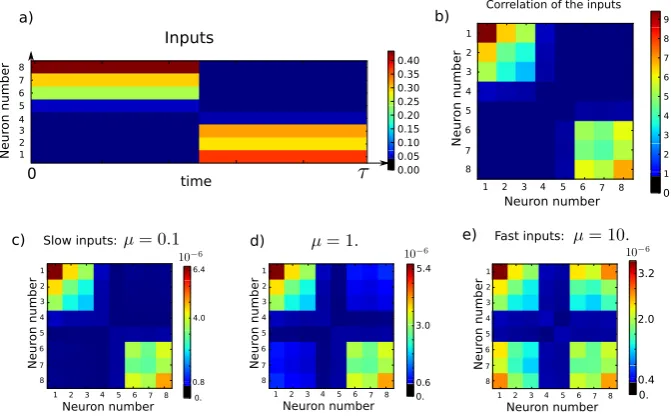
Proof See TheoremB.5in AppendixB.2. At the first order, the final connectivity isC0,0, the filtered correlation of the inputs convolved with a bell-shaped centered temporal profile. In the case of Figure3, this is quite a good approximation of the final connectivity.
Not only the spatial correlation is encoded in the weights, but there is also some information about the temporal correlation,i.e., two successive but orthogonal events occurring in the inputs will be wired in the connectivity although they do not appear in the spatial correlations; see Figure3for an example.
3.3 Trace learning: band-pass filter effect
In this section, we study an improvement of the learning model by adding a certain form of history dependence in the system and explain the way it changes the results of the previous section. Given that Theorem2.2only applies to an instantaneous process, we will only be able to treat the history-dependent systems which can be reformulated as instantaneous processes. Actually, this class of systems contains models which are biologically more relevant than the previous model and which will exhibit interesting additional functional behaviors. In particular, this covers the following features:
• Trace learning.
It is likely that a biological learning rule will integrate the activity over a short time. As Földiàk suggested in [27], it makes sense to consider the learning equation as being
dW
dt = −κW
+v∗g 1
⊗v∗g1
,
Fig. 3 (a) shows the temporal evolution of the input to an=8 neurons network. It is made of two spatially random patterns that are shown alternatively. (b) shows the correlation matrix of the inputs. The off-diagonal terms are null because the two patterns are spatially orthogonal. (c), (d), and (e) represent the first order of Theorem3.5expansion for differentμ. Actually, this approximation is quite good since the percentage of error between the averaged system and the first order, computed by error=W−order 11
W1 , have an order of magnitude of 10−4% for the three figures. These figures make it possible to observe the role ofμ. Ifμis small,i.e., the inputs are slow, then the transient can be neglected and the learned connectivity is roughly the correlation of the inputs; see (a). Ifμincreases,i.e., the inputs are faster, then the connectivity starts to encode a link between the two patterns that were flashed circularly and elicited responses that did not fade away when the other pattern appeared. The temporal structure of the inputs is also learned whenμis large. The parameters used in this figure are=0.001,l=12,κ=100,σ=0.02.
learning, makes it possible to perform invariant object recognition. Besides, trace learning appears to be the symmetric part of the biological STDP rule that we detail in Section3.4.
• Damped oscillatory neurons.
Many neurons have an oscillatory behavior. Although we cannot take this into account in a linear model, we can model a neuron by a damped oscillator, which also introduces a new important time-scale in the system. Adding adaptation to neuronal dynamics is an elementary way to implement this idea. This corresponds to modeling a single neuron without inputs by the equivalent formulations
dv dt = −lz
,
dz
dt =β2(v
−z) ⇔
dv dt = −lv
∗g 2,
whereg2(t )=β2e−β2tH (t ).
• Dynamic synapses.
section, we consider that each synapse is a linear filter whose finite impulse re-sponse (i.e., the post-synaptic potential) has the shapeg3(t )=β3e−β3tH (t ). This is a common assumption which, for instance, is at the basis of traditional rate based models; see Chapter 11 of [7].
For mathematical tractability, we assume in the following that β=β1=β2=
β3∈R+such that gβ =g1=g2=g3,i.e., the time-scales of the neurons, those of the synapses and those of the learning windows are the same. Actually, there is a large variety of temporal scales of neurons, synapses, and learning windows, which makes this assumption not absurd. Besides, in many brain areas, examples of these time constants are in the same range (10 ms). Yet, investigating the impact of breaking this assumption would be necessary to model better biological networks. This leads to the following system:
dv=11((W−L)·v∗gβ+u(2t )) dt+√σ1 dB(t ), dW
dt = −κW
+(v∗g
β)⊗(v∗gβ),
(16)
where the notations are the same as in Section3.2. The behavior of a single neuron will be oscillatory damped if=
1−4βl is a pure imaginary number,i.e., 4l > β. This is the regime on which we focus. Actually, the Hebbian linear case of Section3.2 corresponds toβ= +∞in this delayed system.
To comply with the hypotheses of Theorem2.2(i.e., no dependence of the history of the process), we can add a variablezto the system which takes care of integrating the variablevover an exponential window. It leads to the equivalent system (in the limitσz→0)
⎧ ⎨ ⎩
dv
z
= 1 1
0W−L
β −β
v
z
+u(t 2)
0 dt+
√σ 1dB(t ) σz √
1dB(t )
,
dW
dt = −κW
+z⊗z.
This trick makes it possible to deal with some history-based processes where the dependence on the past is exponential.
It turns out most of the results of Section3.2remain true for system (16) as de-tailed in the following. The existence of the solution onR+is proved in TheoremB.6. The computations show that in the averaged system, the noise term remains identi-cal, whereas the correlation term is to be replaced by μτ(v¯∗gβ)·(v¯∗gβ). Besides, Lemma3.2can be extended to our delayed system by changing only the temporal filters; see LemmaB.7. Together with LemmaC.3, this proves the result of Theo-remB.8.
μ
τ(v¯∗gβ)·(v¯∗gβ)
=u2mv21
l2
+∞
k,q=0 Wk
(l/v1)k · ˜
Ck,q· W
q
(l/v1)q
,
where
˜
Ck,q= 1
u2 mτv
k+q+2 1