Robotic Arm Control Using Pid Controller And Inverse Kinematics

(1)

IJEDR172247

International Journal of Engineering Development and Research (www.ijedr.org)

1571

Robotic Arm Control Using Pid Controller And

Inverse Kinematics

Ms. Vaijayanti B.1

1_{PG, Dept of Mechanical, NIE, Mysore}

Abstract: Space robotics has been considered one of the most promising approaches for on-orbit services such as docking, berthing, refueling, repairing, upgrading, transporting, rescuing, and orbit cleanup. Many enabling techniques have been developed recently and several technology demonstration missions have been completed. All of the accomplished unmanned technology demonstration missions were designed to service perfectly known and cooperative targets only. Servicing a non-cooperative satellite in orbit by a robotic system is still an untested mission facing many technical challenges. One of the largest challenges would be how to ensure the servicing spacecraft and the robot to safely and reliably dock with or capture the target satellite and stabilizing it for subsequent servicing, especially if the serviced target is unknown regarding its motion and kinematics/dynamics properties. This paper discuss how the robot kinematics are controlled using the PID controller using MATLAB/SIMULINK and ARDUINO software.

Index terms – PID, Brushed DC motor control, Inverse Kinematics

I. INTRODUCTION

The benefits of on-orbit satellite servicing include satellite refuelling, satellite life extension, debris removal, repair and salvage. The robotic systems play an important role in satellite servicing and satellite capture is a critical phase for enabling service operations. In the satellite operations the servicing vessel approaches the target satellite to a distance .Then a robotic manipulator is used to autonomously capture the target satellite and perform the docking operation with the vehicle. Movements of the manipulator disturb the attitude of the satellite carrying it, complicating the kinematics and dynamics analysis of the space manipulator. The workspace is reduced as well. As regards the base spacecraft, three types of operation are considered. The first type corresponds to the free flying case, where the base is actively controlled and hence, the entire servicing system is capable of being transferred and orientated arbitrarily in space. The utilization of such a system may be limited because the manipulator motion can both saturate the reaction jet system and consume large amount of fuel. In the second type, the base attitude is controlled by using reaction wheels, leaving the spacecraft only in free translation.

These two categories are split because in some cases only the control of the attitude change is enough to reach the target position and to avoid loss of communication with ground stations and disorientation of solar panels. The third is the free-floating case, where the attitude control of the base is inactive and thus, the base is completely free to translate and rotate in reaction to the manipulator motion. In general the forward kinematics problem for a space manipulator becomes a dynamic problem with the property that the robot’s end-effector position at the end of a maneuver is not only a function of the final joint angles, but also depending on the time history of the joint angles and the inertial properties of the system. People prefer it to use in different field, such as industry, some dangerous jobs including radioactive effects. They can be managed easily and provides many advantages. In a kinematic analysis the position, velocity and acceleration of all the links are calculated without considering the forces that cause this motion. The relationship between motion, and the associated forces and torques is studied in robot dynamics. Robot kinematics deals with aspects of redundancy, collision avoidance and singularity avoidance. While dealing with the kinematics used in the robots we deal each parts of the robot by assigning a frame of reference to it and hence a robot with many parts may have many individual frames assigned to each movable parts. Each frame is named systematically with numbers. In the kinematic analysis of manipulator position, there are two separate problems to solve: direct kinematics, and inverse kinematics. Direct kinematics involves solving the forward transformation equation to find the location of the hand in terms of the angles and displacements between the links. Inverse kinematics involves solving the inverse transformation equation to find the relationships between the links of the manipulator from the location of the hand in space. Further chapters will discuss step by step implementation of a manipulator.

II. STRUCTURE OF ROBOTIC SYSTEM

(2)

IJEDR172247

1572

Fig 1. :Robotic arm structure

The robotic arm consists of shoulder joints, elbow joints, wrist joints and an end effector. It has 6 rotational degrees of freedom (DOFs), 2 at shoulder, 1 at elbow and 3 at the wrist. The end effector consists of 2 finger gripper. All joints are operated using brushed DC motor and the gripper is operated using stepper motor.

III. DC MOTOR CONTROL IN FEEDBACK LOOP BRUSHED DC MOTOR:

DC brush motors rotate continuously when voltage is applied to their terminals. Rotor, stator, brush and commutator assembly. The rotor has got windings of armature and the stator has got the magnet. The brush and the commutator assemblies switch the current to the armature maintaining an opposed field in the magnets. The selection of the electric drive is based on the torque rating and the current rating of the motor. The torque rating of an electric motor is derived from the power rating of the motor

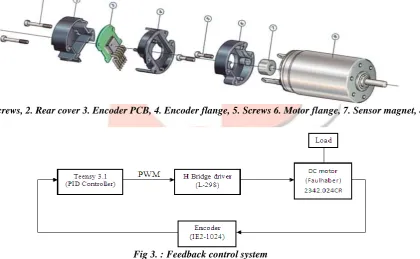
Fig 2. :1. Screws, 2. Rear cover 3. Encoder PCB, 4. Encoder flange, 5. Screws 6. Motor flange, 7. Sensor magnet, 8.Motor

Fig 3. :Feedback control system

The desired position is compared with the actual position feedback from the encoder. This gives the desired speed, which is compared with the actual speed obtained as a feedback from tacho generator. This gives the desired current which is adjusted by the inner loop giving a feedback of actual current. A control signal is generated which along with supply voltage from supply system is given to the motor as input.

Fig 4. :Electrical DC motor model Now lets get the DC motor transfer function. Consider motor torque equation is given by,

(3)

IJEDR172247

1573

Where Kt is torque constant and motor torque is directly relate to armature current. Back emf is related to rotational velocity and is given by ,

e = Ke ∗ θ′ ₍₂₎

By Newton’s 2nd_{law i.e. torque is the rate of change of angular momentum,}

τ = Jθ" + bθ′  K ∗ I = Jθ" + Bθ′ Js2_{∗ θ(s) + bs ∗ θ(s) = K ∗ I(s) (3)} By Kirchoff’s law we get,

I =Va − Vb

L + R LdI

dt + RI = Va − Vb = Va − Ke ∗ θ

′

[Ls + R]I(s) = V(s) − Ke ∗ s ∗ θ(s) (4)

By equations (3) & (4)

Js2_{θ(s) + bsθ(s)}

K =

V(s) − Ksθ(s) Ls + R

s(Js + b)θ(s)(Ls + R) − K ∗ V(s) + K2_{sθ(s) = 0}

So the DC motor tranfer function is given by, ω(s)

V(s) =

K

[(Js + b)(Ls + R) + K2_] which gives speed v/s voltage equation used for speed control of dc motor.

θ(s)

V(s)=

K

s[(Js + b)(Ls + R) + K2_]

which gives angle v/s voltage equation used for speed control of dc motor. Given specifications of brushed DC motor

Nominal voltage 24 V

Armature resistance (R) 7.1 Ω

Back EMF (b)

2.73 𝑚𝑉/ min−1

Torque constant (Kt) 26.1 mNm/A

Armature inductance(L) 265 µH

Inertia of the system (J) 5.8 gcm2

Putting all the values in final equation we get the transfer function of a DC motor as- θ(s)

V(s)=

0.0261

s[1.537 ∗ 10−8_s2_{+ 4.125 ∗ 10}−4_{s + 0.020064]}

Motor Encoder:

Encoder helps us to determine how much motor has moved from its original position. Encoders are of two types; incremental and absolute. Absolute encoders have an index channel to indicate the distance travelled from a fixed point. But in the incremental encoder, there is no such mechanism, we can find out the relative distance between the original position and current position. In this project we are using incremental magnetic encoder. Faulhaber encoders are designed with a diametrically magnetized code wheel which is pressed onto the motor shaft and provides the axial magnetic field to the encoder electronics. The electronics contain all the necessary functions of an encoder including hall sensors, interpolation, and driver.

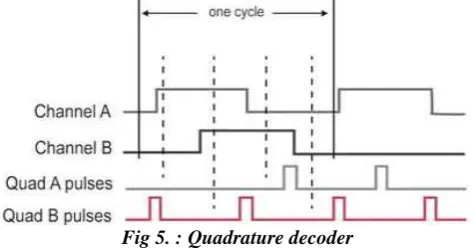
Fig 5. :Quadrature decoder

Depending on which sensor has sensed 1st_{we can predict that in which direction the motor is moving .by counting the}

number of pulses generated by the sensors we can calculate how much angle the motor has moved from the initial position. It can be calculated using the following formula

𝑨𝒏𝒈𝒍𝒆𝒂𝒄𝒒𝒖𝒊𝒓𝒆𝒅= (𝑵𝒖𝒎𝒃𝒆𝒓 𝒐𝒇 𝒑𝒖𝒍𝒔𝒆𝒔) ∗ 𝟑𝟔𝟎

𝒑𝒖𝒍𝒔𝒆 𝒑𝒆𝒓 𝒓𝒆𝒗𝒐𝒍𝒖𝒕𝒊𝒐𝒏

(4)

IJEDR172247

1574

degree. But if we consider the 2nd_{channel counts then our least count becomes 0.17578125 degree. Like this by analyzing the}

channels we can predict the direction of the motor and also it can be used for position detection. IV. PID CONTROLLER FOR ERROR CORRECTIONS

A proportional– integral– derivative controller (PID controller) is widely used in industrial control systems. It is a generic feedback control loop mechanism and used as feedback controller. PID loop defines how much energy is to be fed to the motor at any instant during a move. This is based on where the motor is and where it was expected to be. There are four parts in the equation and determines this load in which three main components are referred to as the P, I, D and the minor friction component is referred to as K.

Fig 6. :PID loop control system

P determines the reaction to current error, I determine reaction to the sum of recently appeared errors, and D determines reaction according to the rate off error changing. The sum of all three parts contribute the control mechanism such as speed control of a motor in which P value depends upon current error, I on the accumulation of previous error and D predict future error based on the current rate of change. There are many PID tuning methods few are discussed here.

i. Ziegler–Nichols tuning method

PID general formula

G1 = Kp +Ki

s + Kd ∗ s => 𝐺1 =

Kd [s2₊Kp

Kd∗ s +

Ki Kd] s

Second order transfer function equation

G2 = ω

2

s2_{+ 2εωs + ω}2 By comparing the G1 and G2 equations we get

ω2₌ Ki

Kd and 2ωε = Kp Kd

By assuming Kp=1, and ω=0.16155 (by the DC motor equation ) ,we can calculate the values of Ki and Kd as 0.080775 and 3.09501.

PLANT PID parameters

𝜀 & 𝜔 Kp Ki Kd

1 0.080775 3.09501

Tuning limits

1 𝜖𝜔

2𝜀

𝛼 2𝜀𝜔

𝜖 = 0.05 𝛼 = 0.386

0.00403875 1.19671

Table 1:Gain calculations using Z-N method

Controller Kp Ki Kd

P T

L

0 0

PI 0.9T

L

0.27T L2

0

PID 1.2T

L

0.6T L2

0.6T

Table 2: Z-N tunning parameters

(5)

IJEDR172247

1575

By simulating the obtained values calculate the values of L and T . The first iteration values calculated are L=2.3 ,T=5.7 then KP= 2.9739 ,Ki =0.64650, Kd=3.42 .Then the 2nd_{iteration values are Kp =2.56, Ki =0.853,Kd=1.92 where L=1.5 and T=3.2 The}

simulation results shows both block response of MATLAB.

ii. Pole Placement Method:

Consider a plant described by its transfer function

𝐺(𝑠) =𝑁(𝑠)

𝐷(𝑠)𝑒

−𝑠𝐿

Where N(s)/D(s) is a proper and co prime rational function .A PID controller in the form of

𝐶(𝑠) = 𝐾𝑝 +𝐾𝑖

𝑠 + 𝐾𝑑 ∗ 𝑠

Is used in the plant with unity feedback in closed loop system

1 + 𝐶(𝑠)𝐺(𝑠) = 0 The closed loop transfer function is

𝐻(𝑠) = [𝑁(𝑠)(𝐾𝑑𝑠

2_{+ 𝐾𝑝 ∗ 𝑠 + 𝐾𝑖)]}

[𝐷(𝑠)𝑠 + 𝑁(𝑠)𝑒−𝐿𝑠_{(𝐾𝑑𝑠}2_{+ 𝐾𝑝 ∗ 𝑠 + 𝐾𝑖)]}𝑒

−𝐿𝑠

𝐾𝑖 =𝑎

2_{+ 𝑏}2

2𝑎 𝐾𝑝 − (𝑎

2_{+ 𝑏}2_)𝑥1

𝐾𝑑 = 1

2𝑎𝐾𝑝 + 𝑥2

𝐾𝑝 + 𝐾𝑖

−𝑎 + 𝑏𝑗+ 𝐾𝑑(−𝑎 + 𝑏𝑗) = −

1 𝐺(ρ1) Where :

𝑥1 = 1

2𝑏𝐼𝑚 [ −1 𝐺(ρ1)] +

1 2𝑎𝑅𝑒[

−1

𝐺(ρ1)] and 𝑥2 = 1 2𝑏𝐼𝑚 [

−1 𝐺(ρ1)] −

1 2𝑎𝑅𝑒[

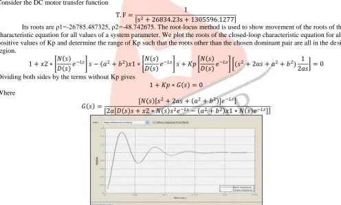
−1 𝐺(ρ1)] Consider the DC motor transfer function

T. F = 1

[s2_{+ 26834.23s + 1305596.1277]}

Its roots are ρ1=-26785.487325, ρ2=-48.742675. The root-locus method is used to show movement of the roots of the characteristic equation for all values of a system parameter. We plot the roots of the closed-loop characteristic equation for all the positive values of Kp and determine the range of Kp such that the roots other than the chosen dominant pair are all in the desired region.

1 + 𝑥2 ∗ [𝑁(𝑠)

𝐷(𝑠)𝑒

−𝐿𝑠_{] 𝑠 − (𝑎}2_{+ 𝑏}2_{)𝑥1 ∗ [}𝑁(𝑠)

𝐷(𝑠)𝑒

−𝐿𝑠_{] 𝑠 + 𝐾𝑝 [}𝑁(𝑠)

𝐷(𝑠)𝑒

−𝐿𝑠_{] [(𝑠}2_{+ 2𝑎𝑠 + 𝑎}2_{+ 𝑏}2₎ 1 2𝑎𝑠] = 0 Dividing both sides by the terms without Kp gives

1 + 𝐾𝑝 ∗ 𝐺(𝑠) = 0 Where

𝐺(𝑠) = [𝑁(𝑠)[𝑠

2_{+ 2𝑎𝑠 + (𝑎}2_{+ 𝑏}2_)]𝑒−𝐿𝑠_]

[2𝑎[𝐷(𝑠)𝑠 + 𝑥2 ∗ 𝑁(𝑠)𝑠2_𝑒−𝐿𝑠_{− (𝑎}2_{+ 𝑏}2_{)𝑥1 ∗ 𝑁(𝑠)𝑒}−𝐿𝑠_]]

Fig 8. :Simulation of PID tuned values using Pole placement method

If we want overshoot be less than 5% and to improve the rising time to less than 2.5sec then use Kp=50 and calculate the remaining gain values. In this case we will get it as Ki=-2406.44 and Kd=-1.012 and respose time is 0.0234. By comparing both the tuning methods we can see that Pole placement method has quick response time than Z-N method. These obtained values are then entered into ARDUINO code.

V. ROBOT KINEMATICS

(6)

IJEDR172247

1576

find the location of the hand in terms of the angles and displacements between the links. Inverse kinematics involves solving the inverse transformation equation to find the relationships between the links of the manipulator from the location of the hand in space. In the next chapters, inverse and forward kinematic will be represented in detail. Homogeneous transformation is used to solve kinematic problems. This transformation specifies the location (position and orientation) of the hand in space with respect to the base of the robot, but it does not tell us which configuration of the arm is required to achieve this location. Inverse kinematics is the opposite of forward kinematics.

In contrast to the forward problem, the solution of the inverse problem is not always unique: the same end effector pose can be reached in several configurations, correspond position vectors. Although way more useful than forward kinematics, this calculation is much more complicated too. The joint structure of a robot can be described by a string such as “RRRRRR” for the Puma and “RRPRRR” for the Stanford arm, where the jth character represents the type of joint j, either Revolute or Prismatic. A systematic way of describing the geometry of a serial chain of links and joints is known today as Denavit-Hartenberg notation. For a manipulator with N joints numbered from 1 to N, there are N +1 links, numbered from 0 to N. Link 0 is the base of the manipulator and link N carries the end- effector or tool.

Fig 9. :Definition of standard Denavit and Hartenberg link parameters.

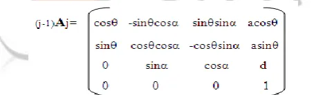
Joint j connects link j −1 to link j and therefore joint j moves link j. A link is considered a rigid body that defines the spatial relationship between two neighboring joint axes. A link can be specified by two parameters, its length aj and its twist αj. Joints are also described by two parameters. The link offset dj is the distance from one link coordinate frame to the next along the axis of the joint. The joint angle θj is the rotation of one link with respect to the next about the joint axis. The coordinate frame {j} is attached to the far (distal) end of link j. The axis of joint j is aligned with the z-axis. These link and joint parameters are known as Denavit-Hartenberg parameters. Following this convention the first joint, joint 1, connects link 0 to link 1. Link 0 is the base of the robot. Commonly for the first link d1=α1= 0 but we could set d1> 0 to represent the height of the shoulder joint above the base. In a manufacturing system the base is usually fixed to the environment but it could be mounted on a mobile base such as a space shuttle, an underwater robot or a truck. The final joint, joint N connects link N−1 to link N. Link N is the tool of the robot and the parameters dN and aN specify the length of the tool and its x-axis offset respectively. The tool is generally considered to be pointed along the z-axis as shown in Figure. The transformation from link coordinate frame {j − 1} to frame {j} is defined in terms of elementary rotations_ and translations as

Use the manipulator DH parameters and put them in the above matrix which gives the transformation matrices for the manipulator. For example 6DOF manipulator has 6 transformation matrices i.e. 0𝐴1 ,1𝐴2, 2𝐴3, 3𝐴4, 4𝐴5, 5𝐴6. Now using these matrices we can find out kinematics equations of the robotic arm i.e.

0H6=0𝐴1 ∗ 1𝐴2 ∗ 2𝐴3 ∗ 3𝐴4 ∗ 4𝐴5 ∗ 5𝐴6 5H6 =5A6, 4H6 =4A5 * 5H6, 3H6 =3A4 * 4H6

2H6 =2A3*3H6, 1H6 =1A2 * 2H6

Now comparing these kinematic equations with the standard goal point transformation matrix which includes position and orientation of the goal point. This gives the required joint angles for the manipulator.

VI. SIMULATION

(7)

IJEDR172247

1577

Fig 10. :Robotic arm simulation

VII. ROBOT PATH PLANNING

Path Planning is finding an appropriate path for robot movement in an obstacle-free space from the source to the destination. Obstacle-free space is the space of the robot movement which is not located in the configuration space. In this paper, the optimal path is the path which is between the source and destination and has the smallest distance among all possible paths. There are many algorithms to do the robot path planning. Assume that you have a robot arena with an overhead camera. The camera can be easily calibrated and the image coming from the camera can be used to create a robot map. This is a simplistic implementation of the real life scenarios where multiple cameras are used to capture different parts of the entire workspace, and their outputs are fused to create an overall map used by the motion planning algorithms. The same camera can also be used to capture the location of the robot at the start of the planning and also as the robot moves. This solves the problem of localization. Some algorithms are discussed here

a. Rapidly-Exploring random trees (RRT)

The RRT algorithm grows and maintains a tree where each node of the tree is a point (state) in the workspace. The area explored by the algorithm is the area occupied by the tree. Initially the algorithm starts with a tree which has source as the only node. At each iteration the tree is expanded by selecting a random state and expanding the tree towards that state. Expansion is done by extending the closest node in the tree towards the selected random state by a small step. The algorithm runs till some expansion takes the tree near enough to the goal. The size of the step is an algorithm parameter. Small values result in slow expansion, but finer paths or paths which can take fine turns. The tree expansion may be made biased towards the direction of the goal by selecting goal as the random state with some probability. The concept is shown in Figure.

Fig 11. :Simulation result of RRT path planning algorithm

If source= [10, 10] and goal= [490,490] then after execution of the algorithm we get processing time=3.624312e+000, Path Length=8.049527e+002

b. PROBABILISTIC ROAD MAP (PRM)

(8)

IJEDR172247

1578

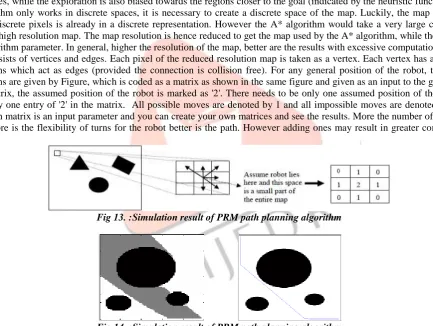
k, better would be the results with a loss of computational time. The algorithm then attempts to connect all pairs of randomly selected vertices. If any two vertices can be connected by a straight line, the straight line is added as an edge.

Fig 12. :Simulation result of PRM path planning algorithm

If source= [10, 10] and goal= [490, 490] then after execution of the algorithm we get processing time=5.904835e+001, Path Length=7.191855e+002.

c. A* SEARCH algorithm

The A* algorithm takes a graph as an input and explores, one by one, all the regions, finding the shortest path from the source to all states in the explored regions. The A* algorithm does that such that all the near regions are explored before the further ones, while the exploration is also biased towards the regions closer to the goal (indicated by the heuristic function). Since A* algorithm only works in discrete spaces, it is necessary to create a discrete space of the map. Luckily, the map taken as an array of discrete pixels is already in a discrete representation. However the A* algorithm would take a very large computation time on a high resolution map. The map resolution is hence reduced to get the map used by the A* algorithm, while the resolution is an algorithm parameter. In general, higher the resolution of the map, better are the results with excessive computation time. The graph consists of vertices and edges. Each pixel of the reduced resolution map is taken as a vertex. Each vertex has a number of connections which act as edges (provided the connection is collision free). For any general position of the robot, the possible connections are given by Figure, which is coded as a matrix as shown in the same figure and given as an input to the graph. In the coded matrix, the assumed position of the robot is marked as '2'. There needs to be only one assumed position of the robot and hence only one entry of '2' in the matrix. All possible moves are denoted by 1 and all impossible moves are denoted by 0. The connection matrix is an input parameter and you can create your own matrices and see the results. More the number of ones in the matrix more is the flexibility of turns for the robot better is the path. However adding ones may result in greater computational costs.

If source= [10, 10] and goal= [490, 490] then after execution of the algorithm we get processing time=2.083293e+002, Path length=7.754773e+002 . By comparing all the algorithms, which have same path lengths for the same start and goal point but the processing time differs. So we can say that RRT algorithm is more feasible because it has low computational cost and it is to analyse.

VIII. MATRUINO INTERFACING

(9)

IJEDR172247

1579

Fig 15. :MATLAB -GUI - ARDUINO serial communication

IX. CONCLUSION

This paper shows all the simple and best possible algorithms for the control of robot kinematics and PID tuning methods for system stability using MATRUINO interfacing.

REFERENCES

[1]. Peter Corke, “Robotics,Vision and Control Fundamental Algorithms in MATLAB®”, Springer Tracts in Advanced Robotics Volume 73

[2]. Ganesh S. Hegde, “Industrial Robotics”,RVCE, Mysore.

[3]. Gihan Nagib and W. Gharieb, “Path Planning for a mobile robot using Genetic Algorithms”. [4]. J. C. Latombe, "Robot Motion Planning", Norwell,MA: Kluwer, 1991.

[5]. Prof. Alessandro Francesconi, “Design of a Robotic Arm for Laboratory Simulations of Spacecraft Proximity Navigation and Docking”.