The calculation, scattering and stability of topographic rossby waves

(1)

T h e ca lcu la tio n , sc a tte r in g and

sta b ility o f to p o g ra p h ic

R o ssb y w aves

P h D T h esis

Gavin A nthony Schmidt

D ep artm en t o f M a th em a tics

U n iv ersity C ollege London

U N IV E R SIT Y OF LO N D O N

7'1'V

(2)

ProQuest Number: 10016754

INFORMATION TO ALL USERS

The quality of this reproduction is dependent upon the quality of the copy submitted. In the unlikely event that the author did not send a complete manuscript and there are missing pages, these will be noted. Also, if material had to be removed,

a note will indicate the deletion.

uest.

ProQuest 10016754

This work is protected against unauthorized copying under Title 17, United States Code. Microform Edition © ProQuest LLC.

ProQuest LLC

789 East Eisenhower Parkway P.O. Box 1346

(3)

A b stract

This thesis discusses the calculation and properties of topographic Rossby

waves in homogeneous and continuously stratified rotating flow. These waves

exist due to variations in the background potential vorticity arising from changes

in topography or rotation.

The first part considers the calculation of the frequency and wavenumber

of trapped topographic Rossby waves over various types of topography - along

a coastal shelf (giving coast ally trapped waves), over a submerged ridge and

around an axisymmetric sea mount. A new direct method of calculation in the

low frequency continuously stratified case is introduced. This uses a Green’s

function to reduce the problem to a one dimensional integral across the shelf.

Asymptotic expansions in the stratification param eter B = N D j f L , where N

is the buoyancy frequency, D a typical depth, L a typical length and / the

Coriolis param eter are presented. Both strong stratification (.5 1) and weak

stratification ( B 1) are treated in this fashion and approximations th at are

accurate for all B are constructed for certain simple topographies.

The circumstances th at can lead to singularities appearing in the solution are

investigated and the consequences for general circulation models discussed.

The numerical method is applied to the solution of scattering problems as the

topography changes and to determining the wind-forced response. An isobath

tracing result is used to calculate the distribution of energy among the trans

m itted waves. Examples are given using various geometries including straits and

ridges abutting a coastal shelf.

The stability of horizontal shear flow to small disturbances is considered.

These disturbances have the form of topographic Rossby waves. Unstable modes

can occur over ridges. Detailed examples are worked out in the barotropic case

and in the continuously stratified long-wave case. In both cases the instabilities

are centred at points where the shear flow brings two opposing waves relatively

(4)

C hapter 1

(8)

The study of the weather and of the movement of the oceans has long fasci

nated scientists but it has only been in the last hundred years or so th at much

m athem atical headway has been made. The full processes involved in shaping

the flow are, in the main, still poorly understood but a great deal of the global

circulation can be well approximated by relatively simple models. The two ef

fects which distinguish the study of these complex phenomena from other related

disciplines are the rotation of the earth and the stratification of the atmosphere

and oceans by tem perature and salinity.

The recognition of the part tem perature and density play in the circulation

of the atmosphere was recognised by Hailey (1686). He hypothesised th at the

lower density of hot air at the tropics compared with cold air at the poles would

induce a circulation of hot air rising at the tropics, moving polewards, descending

and cooling and returning to the tropics to be reheated. This model did not

however adequately account for the easterly component of the trade winds. The

explanation for this was given by Hadley (1735). Because of the rotation of the

earth, air moving towards the equator from the poles has less angular m om entum

than th at required for a rigid rotation at the equator. Hence air travelling south

gains a westward velocity relative to an observer rotating with the earth. This

model for the circulation is now called a “Hadley cell” . This however, is not seen

in practice for reasons discussed later.

The analytical starting point for the whole subject of fluid dynamics was the

writing down of the equations of motion for an inviscid fluid by Euler (1755).

The appropriate equations for flow in a rotating frame were used by Laplace

(1778,1779) in his work on tides. The implications of the extra term s in the

equations were also discussed by Coriolis (1835) after whom they are now named.

Proudm an (1916) and Taylor (1917) were the first to discuss the importance

of topography in rotating flow. They proved th at in an inviscid, homogeneous,

rapidly rotating flow the streamlines are independent of depth. Hence if flow has

to move around an obstacle at one depth then the streamlines will follow the

same pattern at all depths! This phenomena is known as a “Taylor column” or

(9)

(1923) where he towed an object slowly through fluid in a rotating tank and

observed a stagnant column of water above the object and moving with it.

The modern study of geophysical fluid dynamics though, really started with

the work of Rossby in the 1930’s. In a non-rotating flow a disturbance in the

free surface quickly adjusts to the equilibrium of zero flow and a flat surface.

However Rossby (1937,1938) showed th at the analogous process in a rotating

flow leads not to a static position but to a dynamic balance between the term s

representing the Coriolis force and the pressure gradient. This is now called the

“geostrophic equilibrium” and it is found to approximate the actual situation in

the atmosphere and oceans over a remarkable percentage of the globe.

He also found th at simply knowing th at a fluid is in geostrophic equilibrium

is not enough to determine the flow. Due to a degeneracy in the equations of

motion some account must be taken of small departures from geostrophy. This

led Rossby to discover the principle of the conservation of “potential vorticity” .

For the simplest case of homogeneous inviscid incompressible rotating flow this

principle can be expressed very simply. If ( is the relative vorticity of the flow,

/ the Coriolis frequency and h the depth of fluid then

where D / D t is the m aterial derivative or “rate of change following the fluid” .

The quantity in brackets is called the potential vorticity(PV) and this equation

shows th at it is conserved for every fluid element. Hence a knowledge of the

initial PV field of a fluid in geostrophic equilibrium is sufficient to determine the

subsequent flow.

There are some other im portant consequences of this conservation law. On

the earth, both the Coriolis frequency and the depth of the ocean or atmosphere

vary from place to place. Hence so does the background PV { f / h ) . If a column

of fluid moves from an area of high background PV to one of low background PV

then the conservation law requires that the relative vorticity must increase. But

this anti-clockwise rotation in turn forces adjacent fluid columns to move in such

a way as to restore the column to its original level but slightly to one side. It will

tend to overshoot due to inertia and an oscillation will develop which will always

(10)

topo-graphie or planetary Rossby waves depending on whether change in topography

or variation of the Coriolis frequency is the main restoring mechanism.

Lord Kelvin (Thompson, 1879) also investigated the properties of waves in

rotating fluids. In particular, he found th at wave motions were possible in the

presence of a side boundary and a flat bottom . These “Kelvin” waves arise as a

balance between the Coriolis acceleration and gravity on the surface and satisfy

the same dispersion relation as external gravity waves, i.e.

w = kyfgD, (1.2)

where D is the depth of fluid, w is the frequency and k the wavenumber. The

distance th at the Kelvin wave extends out to sea is 0(rg) = 0 { \ / g D / f ) . This

length is called the Rossby radius of deformation and it is an indication of distance

over which the tendency of gravity to flatten the surface is balanced by the

tendency of rotation to deform it. These waves, in common with Rossby waves,

are unidirectional and always travel with the boundary to the right.

Stratification, whether due to tem perature differences or salinity, adds an

im portant dimension to the range of possible wave motions. One way of charac

terising the strength of the stratification in a fluid is to consider the frequency

of oscillation of a fluid element displaced vertically from its equilibrium position.

Brunt (1927) and Vaisala (1925) introduced the idea of this buoyancy frequency,

sometimes known as the Brunt-Vaisala frequency, which is a function of depth

and can be w ritten

where p{z) is the equilibrium density distribution. The larger is, the more

stable the fluid. A negative implies th at the fluid is unstable i.e. lighter fluid

lying under heavier fluid.

The concept of potential vorticity, which is only really an expression of angular

m om entum divided by the volume, can be extended to stratified flow. It is

straightforward in the linear cases and the general form was given by Ertel (1942).

The quantity th at is conserved is then called E rtel’s potential vorticity. It has

many of the same qualities as the potential vorticity mentioned above and reduces

(11)

In non-rotating flow stratification allows for the propagation of internal grav

ity waves and in rotating flow it allows “internal” Kelvin waves to propagate

along a side boundary. These are similar in structure to the “external” Kelvin

wave discussed above but have a sinusoidal structure in the vertical. Unlike the

external Kelvin wave though, these do not require a displacement in the free sur

face to exist. If the buoyancy frequency, N, is constant they satisfy the dispersion

relation

(V = ,n = 0 , l , 2 . . . , (1.4)

OLn

where a„ are the solutions of a tan a = N^D/g. These waves have a length scale

out to sea of 0 { N D / f ) which is usually much smaller than the Rossby radius,

Te- In general, stratification reduces vertical movement and inhibits the vertical

transmission of information. It also increases the horizontal speed of the waves.

In the vicinity of a coastal or continental shelf there are very large variations of

depth. Because of the changes in the background potential vorticity, topographic

Rossby waves would be expected to propagate along such a shelf. But, due to

the stratification of the ocean at such a sharp change of depth, Kelvin waves

would also be expected. Both types of wave are unidirectional and travel with

the shelf to their right. Robinson (1964) considered the homogeneous problem

and christened these waves “continental shelf waves” or “coastal trapped waves” .

They are “trapped” in the sense th at, if the variation of the Coriolis frequency

with longitude is negligible, there is no mechanism capable of transm itting energy

away from the coastal wall and out to the open ocean. More grammatically

perhaps, they are described as “coastally trapped waves” in later papers and in

the remainder of this thesis.

Stratification can be added to this model in a number of ways. Allen (1975)

and Mysak (1967) used various two-layer models while Wang and Mooers (1976)

and subsequent authors used continuous stratification based on the concept of

the buoyancy frequency These continental shelf waves combine aspects of

both Kelvin waves and topographic Rossby waves, and it is only in extreme cases

th a t there is a clear distinction between the two limiting forms. The param eters

determining the structure of the waves are simply the ratio of the topographic

(12)

scales. These are the “Burger” number B = N D / f L and the ratio a = r^ /L

and will appear throughout this thesis. For depth profiles where L <C N D / f the

shelf topography is unim portant and all waves are essentially baroclinie Kelvin

modes.

The lack of analytical results has led to attention being focused mainly on nu

merical schemes to determine the frequency and structure. Huthnance (1978) and

Brink and Chapman (1986) both developed two-dimensional grid methods to find

these modes as functions of wavenumber, stratification and topography. A differ

ent approach (Middleton and W right,1990, Johnson,1991) is to use asymptotic

expansions in B to find analytic results in certain extreme param eter regimes and

for simple topographies. The work in Chapter 2 extends the use of asymptotic

expansions to both extremes of B and provides approximations th at are valid for

B of order one.

A new numerical method is also introduced in the long-wave continuously

stratified case. This uses a Green’s function to reduce the two-dimensional partial

differentiation problem to a one dimensional integral on the shelf. This greatly

increases the accuracy and efficiency of the numerics over previous methods. The

correlation between the numerics and the asymptotics is very good.

In a two-layer model, where there is a forced separation between the modes,

Allen found th at the different modes can “kiss” as the stratification changes.

This occurs as the speed of the Kelvin wave approaches th at of the first topo

graphic mode. Instead of crossing they kiss and exchange characteristics. This

is confirmed by the new numerical method but is found to occur only in some

rather special cases.

Of course, these types of wave relying on both topography and stratification

are not unique to coastal shelves. The same analysis can be applied to sub

merged ridges such as a mid-ocean scarp or to isolated features such as seamounts.

Longuet-Higgins (1968) called the modes over a scarp “double Kelvin waves” and

Rhines (1969a,b) considered the extension to isolated seamounts and other to

pography. In Chapter 3 similar analysis for the stratified case is performed and

the numerical method extended for the infinite ridge case.

A complication arises as the stratification increases due to a singularity ap

(13)

in §3.2 shows th at the relevant governing equation in the immediate vicinity of

a corner is the two-dimensional Laplace equation. If there is no influence from

the other boundaries then the classical singular solution at a corner is valid. The

boundaries will not influence the solution there if the vertical scale of the motion

( f L / N ) is much less than the depth i.e. B ^ 1. Some methods of solution

however are not affected by the singularities. An example in §3.3 uses m atched

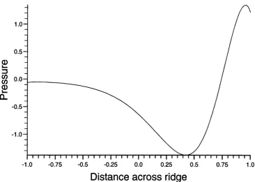
Fourier expansions for a ridge with a top-hat stepped profile. The sharp peak in

the pressure gradients predicted arises even for quite m oderate values of B.

This has implications for General Circulation Models (GCMs) th at use sim

plified step topography. In §3.4 an example (Sherwin and Dale, 1992) of the

inaccuracy of these models is shown. The frequency of a TRW around a sea

mount is found semi-analytically using the same methods as in §3.3 and the

results are analysed and compared to the output from a GCM. The model in

troduces large errors at the corners which lead to significant inaccuracies in the

calculation of the frequencies of the waves.

There are two main problems to which this method has been profitably ap

plied, the scattering of low-frequency energy as the topography changes (Johnson,

1989a) and the response of coastal waters to applied wind stress (Clarke and van

Corder, 1986). These theories rely mainly upon the orthogonality of the wave

modes and only use the values of the pressure on the shelf. The numerical m ethod

introduced in §2.4 calculates only these values and has a much greater resolution

on the shelf than was previously available. The modes calculated are also much

closer to orthogonality. In §4.2 the isobath tracing result of Johnson (1989) is

derived and some simple examples given.

The field of coastally trapped waves in the vicinity of East Australia has

attracted a lot of attention since Hamon (1966) first detected their presence.

More systematic observations made in the Australian Coastal Experiment (ACE)

and reported by Freeland et al (1986) indicated th at contrary to expectation

significant amounts of low-frequency energy were emerging from the Bass Strait

in form of CTWs. W hether these waves arise from wind forcing within the

Strait itself or are transm itted waves th at originated along the Great Australian

Bight has been discussed by (among others) Buchwald and Kachoyan (1987) and

(14)

by considering the scattering of CTWs through generalised straits by solving

the barotropic equations. In §4.3 the isobath tracing result is applied to this

geometry and magnitudes of the scattered modes are found without having to

explicitly find the solution within the strait.

Another example, considered by Killworth (1989a,b) and Johnson (1989b,

1993) is the scattering caused by a ridge abutting a coastal shelf. Energy can

either continue along the coast or be transm itted down the ridge. This more

complicated question is tackled in §4.4.

Equations governing the CTW response to wind forcing were derived by

Clarke and Van Corder (1986) who used the orthogonality of the free modes

to get a simple first order partial differential equation for the amplitudes. In

practical applications of this theory Lopez and Clarke (1989) and Brink (1991)

found th a t a large number of higher modes (up to 30) were needed to specify the

alongshore velocities. This was previously impractical. The new m ethod on the

other hand accommodates accurate representation of these higher modes with

ease. In §4.5 a simple example using harmonic wind stress is given to show the

convergence of the pressure and alongshore velocity as more modes are added.

The crucial question concerning all hypothetical models is whether they bear

any reference to actual motions in the oceans or atmosphere. The answer to th at

lies in the stability of the flow. Helmholtz (1888) recognised th at instabilities

would be im portant in causing vertical mixing and billow clouds in the atm o

sphere but it was Bjerknes (1937) who realised th at the Hadley cell would be

unstable to small longitude-dependent disturbances and so could not persist. In

stabilities in geophysical flow have been divided up into two main categories, the

baroclinie instability which is associated with vertical variations in the velocity

and barotropic instability which is associated with horizontal variations. Because

of the implied vertical shear in the Hadley cell, it would fall victim to baroclinie

instabilities. M athematical models for baroclinie instabilities were developed by

Charney (1947) and Eady (1949). Barotropic instabilities were first considered by

Rayleigh (1880) (in the non-rotating case) but their relevance to geophysical flow

was only recognised by Lorenz (1972) who considered the stability of planetary

Rossby waves in a westerly current.

(15)

are stable. Huthnance (1978) showed th at all coastally-trapped waves over a

monotonie shelf with no background current are stable. Some calculations with

different barotropic currents along a shelf were done by Collings and Grimshaw

(1986). They found th at some shear flows were made unstable by the topography

but th at most instabilities were just modifications of instabilities th at would exist

even without topography.

The more interesting case concerns a barotropic shear flow over a ridge. W ith

no shear, waves can exist on both sides of a ridge and travel in opposite direc

tions. The addition of the shear has two main effects: it changes the background

potential vorticity upon which these waves depend and it advects the waves. This

leaves the possibility th at some waves will now travel in the opposite direction

and, more im portantly for the question of stability, th at two waves on opposite

sides of the ridge might be brought relatively to rest. As in Taylor (1931) who

considered the instability of three layer stratified flow, this can be one of the

main preconditions for instabilities to occur.

In the homogeneous limit the problem has a particularly simple form in terms

of the barotropic streamfunction. Some necessary conditions for instability to

occur are derived in §5.2 and some examples using linear shear are given in §5.4.

The equations are also tractable in the long-wave low-frequency lim it for the

stratified case, §5.3.

These models are only approximately true for real flows. In the real world

viscosity, friction, compressibility, therm al effects etc., all play a part in the

overall flow. In this thesis it is assumed (except in §4.5) a priori th a t these

effects are negligible and th at the fluid is always incompressible i.e. th a t density

is conserved by each fluid element. These assumptions are valid for most of the

medium to large scale motions in the ocean.

In all the analysis th at follows some common assumptions concerning the

density and pressure are made. Firstly th at the density and pressure fields are

perturbations of their hydrostatic or equilibrium values. They can then be w ritten

p* = pq[z)-\-p{Xj t) and p* = po(^)+p(x, t) where the hydrostatic quantities satisfy

poz = —gPO’ The second assumption is known as the “Boussinesq” approximation

following Boussinesq (1903). In the horizontal momentum equations it is assumed

(16)

the vertical momentum equations where p is multiplied by full account of the

departure from the equilibrium position is taken. The variation with depth of po

allows the introduction of the buoyancy frequency N^{z) in the density equation.

This is generally valid in the oceans where po does not vary from its mean by

more than 2% (Gill, 1982).

The Coriolis frequency / will be assumed constant and equal to 2f2sin^o

where Oq is the base latitude and Q the angular speed of the earth. This is

equivalent to assuming that the longitudinal length scale relevant for the motion

L is much less than R tan 6q where R is the radius of the earth. This is valid for

most oceanic flows outside the tropics.

To simplify further the equations of motion in a rational m anner requires

knowledge of the relative importance of the different terms. This can be found

by non-dimensionalising the equations and making order of magnitude estimates.

In general assume th at the horizontal velocities and lengths can be scaled on

typical values U and L, and th at the vertical length scale is D, the depth of fluid.

So th at the pressure terms should match the Coriolis terms in the horizontal

m om entum equations, the perturbation pressure p is scaled on pofUL to give

Ut + (u.V )u - v = -p^, (1.5a)

(u.V )v + u — —py, (1.56)

and where the tim e scale for the motion has be chosen as 1 / / . It is clear th a t the

importance of the Coriolis terms compared with the inertial term s is measured

by Ro = UI f L the “Rossby” number.

In order th at the perturbation density and pressure are of the same magnitude

in the third momentum equation, the density is scaled on p ofU L /g D . The

validity of the Boussinesq approximation is therefore equivalent to the condition

th a t Ro a^. The scaling of the vertical velocity is determined by the density

equation in order to bring the buoyancy frequency into the equations. Scaling w

(17)

- ^ — wN^ = 0. (1.5(f)

where D / D t in this context is equal to d / dt Ro{udIdx v d I d y B ~ ‘^wdJdz).

This introduces the param eter B = N o D / f L which is a measure of the relative

im portance of the stratification and the rotation. The remaining equation is the

incompressibility condition

U x V y B ~ ^ W z = 0^ (1.5e)

If, in addition, the buoyancy frequency is much greater than the Coriolis fre

quency the hydrostatic approximation will be valid in (1.5c). This is equiva

lent to taking the vertical scale D much less than the horizontal scale L (since

P Nq^ = B ‘^ {D / L Y ) which is valid for almost all geophysical flows.

The density can be eliminated to give the the vertical velocity in terms of the

pressure

The horizontal velocities can all be written in term s of the pressure

\ D

d- 1 U - -Py - -=-Px,

Dt^ I Dt

f \ D

\Dt^

+ 1 j

-

^^P«■

(1-7)

If the flow is such th at Ro <C 1, the “quasi-geostrophic” case, (1.5e) then

gives the leading order governing equation for the motion as

Pxx-^Pyy-\-B

This is the stratified counterpart of (1.1).

Some thought must be given to the boundary conditions on the surface and

over topography. The conditions arise as a consequence of the requirement th at

all fluid particles on the surface or bottom remain there throughout the motion.

Additionally, on a free surface the total pressure must be constant. Therefore on

the bottom z = —h the condition is

(18)

On a free surface z = rj, the equivalent condition is th at

- 77) = RoB~^w - ^ = 0, {z = 7}) (1.10a)

Integrate the hydrostatic relation over the depth and use the fact th at the total

pressure is constant on 2; = 77 to get

^ ~ ~ 77) (1.106)

Combine equations (1.10a,b) and assume th at the disturbance of the free surface

is small. Linearise about z = 0 and integrate along the surface to get

+ B ^ N i O f p = 0, {z = 0) (1.11)

The equations (1.8), (1.9), (1.11) form the basis for most of the work in this

thesis. The scalings used are not always identical depending of course on the

particular problem. The homogeneous equations (and 1.1) which are derived

assuming a constant density can be recovered from the above by letting B ^ 0

and expanding in an asymptotic series in powers of B^.

To summarise the assumptions made so far; i) L <C .Rtan ^0, ü) Ro <C a^ and

iii) B ^ { D / L y = { f / N o Y <C 1. In the oceans the depth D ranges from l-5 k m and

in the m id-latitudes {6q > 25°) the magnitude of the Coriolis frequency ranges

from 7x10“ ®5"^ to 1.4xlO“‘^5“^ at the poles. Hence the Rossby radius takes

values ranging from 10,000km in the deep ocean to 150km in coastal waters.

The motions in this thesis will therefore be assumed to have horizontal length

scales much greater than the depth but satisfying the first condition, around

lOO-lOOOkm. The Rossby number will generally be small and in a number of

examples given later the Rossby radius will be taken as infinite, the rigid lid

limit. Care though, must be taken in this limit because of the effect it has on

(19)

C hapter 2

(20)

§2.1 In trod u ction

This chapter concentrates upon the possible wave motions in coastal shelf

regions. Large potential vorticity gradients coexist with significant amounts of

stratification in such regions and hence both the topographic and buoyancy effects

must be included in a realistic model. There is observational evidence for these

waves in m idlatitudes (see Mysak (1980) for a review) which suggests th at they

have periods of several days or more (compared with a Coriolis period of about

1/2-1 day). This implies th at analysis in which the frequency of the waves is

much smaller than the Coriolis frequency will still give physically meaningful

results.

In the low-frequency/long-wave limit, Clarke (1976) showed th at th at waves

are non-dispersive i.e. th at the energy travels with the phase velocity, and th at

this lim it is consistent with theories of atmospheric forcing by pressure systems

with similar periods.

In addition to the barotropic shelf waves (BSWs) obtained by Robinson

(1964), two-layer models allow the propagation of an internal Kelvin wave (IKW).

An interesting feature of the results in Allen (1975) is the observation th a t, as

stratification or alongshore wavenumber increase and the speeds of the internal

Kelvin wave and barotropic waves approach each other, the modes “kiss” and

exchange character. One mode deforms into the other over a very small range of

B. The conditions for which this coupling occurs are discussed in §2.5.

For the continuously stratified case, Huthnance (1978) shows th at there exists

a countable infinity of discrete modes with frequencies < / decreasing to zero.

All modes travel in the same direction (A; > 0) and form a complete set. All

pressure fields are therefore expressible as an infinite series of these modes. The

fundam ental mode is essentially the external Kelvin wave and has maximum

phase speed. If the rigid lid approximation is used however, this mode is filtered

out.

The difficulty of the analytical problem is mainly due to the fact th at the

eigenvalue, w, appears in both the governing equation and boundary conditions

in a non-linear way. Analytical solutions have been found only for extreme pa

(21)

large and small values of the stratification param eter, are obtained, for in

stance by Middleton and Wright (1990) and Johnson (1991). Analysis in §2.2 and

§2.3 show how, in the low frequency limit, this can be systematically extended to

give approximations for the eigenvalues and eigenvectors accurate over the whole

range of B using Fade approximations.

The numerical schemes employed by Huthnance (1978) (inverse iteration) and

by Brink and Chapman (1985) (resonance response to arbitrary forcing term )

while flexible in being able to deal with variable stratification, are indirect m eth

ods th a t require a two dimensional grid over the whole domain. The efficiency

of these methods is reduced by the search procedure necessary and the restric

tion of obtaining only one mode at a time. The new method introduced in §2.4

reduces the problem by analysis from a two dimensional problem to a one dim en

sional eigenvalue problem involving only a line integral across the shelf which can

then be reduced to a series of linear equations. This is done by using a G reen’s

function, G, for the semi-infinite strip and can be used for any shelf topography,

whether it is a piecewise linear approximation or a functional form. If the rigid

lid approximation (a —> oo) is valid and the stratification assumed to be uniform

{N{z) = 1) there is a neat closed form solution for G.

If a free surface or non-uniform stratification is required, G can be found

as an infinite series (Morse and Feshbach, 1953) with only a slight increase in

computing tim e needed.

This method has the advantages both of vastly increased resolution and of

directness and gives all the required modes simultaneously. The resolution of

this m ethod is much greater than in previous models and allows a more detailed

examination of the waves, in particular their scattering is looked at in detail not

previously seen (Chapter 4). Higher modes, as used in theories of wind-forced

long waves (Clarke and Van Corder, 1986), are dealt with much more efficiently

than with previous methods (§4.5).

It is possible to extend this method to higher frequencies but as the frequency

and wavenumber appear non-linearly the search procedure for finding the phase

speed must be changed.

Section 2.5 contains results for various topographies and param eter values

(22)

H

X

y=L

z=0

z=-D

Figure 2.1: The domain A, with the z coordinate vertically upwards, y

increasing out to sea, and x the alongshore coordinate. The width of the shelf is L and the open ocean depth D.

of the numerical method and the analytic asymptotic results confirm the accu

racy of the numerics and of the Fade approximations. The effects of changing

stratification, a free surface and an exponential buoyancy frequency profile are

fully explored.

§2.2 E q uations o f m otion

Consider a semi-infinite ocean of depth D bounded by a monotonie sloping

shelf of width of order L (fig. 2.1). Take Cartesian axes 0 x , 0 y , 0 z along the

shelf, out to sea and vertically with the shelf profile depending on y alone.

Let the flow be Boussinesq and incompressible with uniform Coriolis frequency

/ , total density po{z)-{-p{x, t) and pressure po('Z)+p(x, t). Introduce the buoyancy

frequency scaled with the constant Nq chosen so the maximum value of N{z)

is unity. Use the same scalings as outlined in the introduction and look for

small amplitude waves with (non-dimensional) frequency w and wavenumber k.

Om itting a common factor of exp{iut — ikx) gives from (1.8) the non-dimensional

(23)

-fc"p + p „ + (1 = 0- (2-2.1)

The boundary condition (1.11) at the free surface is

+

B^N\0)p

= 0, (z = 0) (2.2,2) where a = (g D Ÿ '^ / f L , the non-dimensional Rossby radius of deformation. If

z = —h{y) is the profile of the coastal boundary (alternatively y = d(z)) for

2/ < 1, the vanishing of the normal velocity at the boundary implies

{cj/B^)w = —vh'. (z = —h{y)jy < 1)

Substituting in for v , w gives

(1 - w^)cp;g = - h 'B ^ N ^ { p + cpy), {z = - h { y ) , y < 1)

P z = 0, {z = - l , y > l ) (2.2.3)

where c = Lj/k is the phase speed. In the far field (y oo) p -^constant

Now consider the long wave solutions, taking the limit w —^ 0, A; ^ 0 with

c = ujIk fixed. These waves are non-dispersive satisfying (as in Clarke (1976)

and Huthnance (1978) ),

Py y + B - \ N ~ ^ p . ) , = 0, (2.2.4o)

with

h'N^B^{p4- cpy) -f cpz = 0, {z = - h { y ) , y < 1), (2.2.46)

a^Pz + B^N^{0)p = 0, {z = 0), (2.2.4c)

Pz = 0, {z = —l , y > 1). (2.2.4d)

The chief advantage of taking this limit is th at the eigenvalue of the problem,

c, now only appears linearly in the boundary condition.

The standard manipulation using Green’s theorem shows th at the eigenvalues

and eigenfunctions are real, the eigenfunctions corresponding to distinct eigen

values are orthogonal along the slope z = —h{y) and hence can be made or

thonorm al satisfying J^iPnPm dz = 8nm- The eigenfunctions form a complete set

(24)

§2.2.1 Strong stratification {B > 1).

Strong stratification suppresses large vertical motions and from (2.2.4a) in

troduces the dynamically im portant horizontal scale NqD I f , large compared to

the shelf width L. On this scale the shelf appears as an almost vertical wall.

Introduce the long length scale Y = y / B . Then (2.2.4) becomes

PYY + (JV 'V .). = 0, (2.2.5a)

with

B - ^ K d 'p , = N^(p + Kpy) , ( y = B-'^d{z)) , (2.2.56)

+ p = 0, (z = 0), (2.2.5c)

Pz = 0, {z = —1 , Y > 0), (2.2.5d)

where K = B~^c and A = B~^a/N[0). Let be the eigenfunctions and the

eigenvalues for the vertical structure, satisfying

= (2.2.6a)

= 0) > 0)

A Z n = 0 . { z = 0 ) ( 2 . 2 . 6 6 )

Then (2.2.5) has a separated solution of the form

p(y, z) = Z Z„(z) (2.2.7)

n = 0

provided, from (2.2.5b)

oo oo

JV"(z) £ a„(l - KX„)e-’"'<‘^/^Zn{z) = B~^Kd! £ a„e-^”''W/®^;(2). (2.2.8)

71=0 71=0

Expanding ÜT, a„ and Q~>^rid{z)/B terms of B~^ and equating powers of B~^

gives approximate solutions of successively higher order. Explicit examples are

(25)

§2.2.2 W eak stratification ( B <C 1)

For weak stratification w <C ^ 1 the flow is almost barotropic and solutions

follow by expanding (2.2.4) as a series in Bj writing

p{y, z) = + " • (2.2.9a)

c = cq “1“ B^ci -j- B^C2 4" ' ' " (2.2.96)

The expansion proceeds straightforwardly for arbitrary stratification and Rossby

radius, a, but for definiteness N{z) is taken here to be unity and a to be of order

one. Then

= 0. pW = - p ^ - '> , n > 1, (2.2.10a)

p1°^ = 0, (z = 0), n > 1.

p(") = 0, (z = - l , ÿ > l ) , „ > Q . (2.2.106)

The vertical dependence of the pressure field then follows as

= ^o{y),

=

^i{y) - ^z<l)o{y) - ^z^(t>Q{y),

and in general

where the <f>i are functions of y alone. The governing equation for each (f>i comes

from expanding the lower boundary condition (2.2.4b) in B and substituting the

expression (2.2.11) for the pressure terms.

Two boundary conditions are needed in order to solve for the one at

y = 0 and one at y = 1. At y = 0, if there is a finite slope at the origin then the

pressure must be bounded, however if the wall is vertical near the origin, a no flux

condition is necessary, i.e. p + cpy = 0 on y = 0. This condition though, cannot

be satisfied by any order higher than the first. This implies the existence of a

0 { B) boundary layer against the vertical wall. The correct boundary condition

is then no net flux along the wall.

The condition at y = 1 is slightly more problematic. In the rigid lid limit

(26)

boundaries, the vertical line y = 1 — e and which is closed at infinity. The integral

of the normal derivative of p around T is identically zero from Green’s theorem.

Using the boundary conditions, letting B 0 and then letting e —> 0 gives

0

I

^

~ = 1) (2.2.12)

which is satisfied at each order. However for finite a this procedure only provides

a m atching condition to the exponentially decaying solution for y > 1. Change

the circuit T to the lines y = l — e, 2/ = l + e and the top and bottom boundaries,

and follow the same limiting process to get instead of (2.2.12)

= (2.2.13)

A nother matching condition is required to eliminate the outer solution. The net

flux across y = 1 must be equal on both sides and hence

r 0

' = 0. (2.2.14)

y = l J c p y - \ - p dz

L-1

These conditions expanded in a series in B are enough to determine the ^(y) at

all orders. It has been assumed that h{l) = 1, if there is a discontinuity in the

topography the matching conditions can be altered accordingly.

§2.3 A s y m p to tic so lu tio n s

P ro file 1. Let the stratification be uniform, {N{z) = 1), the surface rigid

a ^ 1, and the shelf have the linear profile

^{y) = Vj 2/ < 1 or d{z) = —z, —1 < z < 0. (2.3.1)

a. Strong Stratification

Equations (2.2.6) can be solved readily to give Xn = mr and Zn = y/2cosmrz

normalised so th at

ro f 1, if n = m;

/ ZnZm dz = < (2.3.2)

(27)

Expanding (2.2.8) as indicated with K = Kq-\- B~ ^K i + B ~ ^ K2 + . . . and an =

a° + + . . . for each n, multiplying by Zn and integrating with respect to

Z; gives equations for the eigenvalues and the coefficients a„. The lowest order

equation gives

a ° (l — Komr) = 0, Vn (2.3.3)

If Æo ^ 1/nTT for some n then the solution is identically zero, so for a non

trivial solution, the m th eigenfunction has Kq = Ijm'K with a j = 0 Vr ^ m.

The undeterm ined coefficients can be found by requiring th a t the pressure is

normalised so th at z)dz = 1. Thus the lowest order solution is

p^”'^(2/,z) = cosmTTZ, with speed = j9/m7r, which is pre

cisely the m th mode IKW. The first deviation from this mode is given by the

next term

OO

^ u^(l — Kon7r)cosn7TZ = u^(sin mvrz + üTimTrcosmTrz). (2.3.4)

n = 0

Multiplying by Zm(z) and integrating gives Ki = 0 and multiplying by Zr(z), r ^

m implies

'0 , if m -f r is even;

aj = < —2a^/7rm, if r = 0,m odd; (2.3.5)

^ —4m^a^/7r(m — r)(m^ — r^), otherwise.

This gives the first order solution. The second correction follows from the order

B~^ equation

a^m7r(z sinrnTTZ -h K2 cos mTTz) = ^ ( 1 ---) cos n7rz(a^n7rz-f a^) H a^sinnTrz

n=0 ^ ^

(2.3.6)

as

2m7r § r ^ ( m + n f ( m - n f

n + m o d d

Further terms follow straightforwardly. For the present example the first three

eigenfunctions are

p{y,z) = -s/2 -t- cos mvrz ^ ^ cosn7rz -fO (5 ~^),

n = 0

(28)

3.0-1

2.5

-- -- A pproxim ations — Numerical results

"5 2.0

-Q.

1.5—

1.0

-0.5

-0.0

0.5 1.0 1.5 2.0 2.5

0.0

Stratification(1/B)

F ig u r e 2.2: The comparison of the numerical results and the approxim ate wave speeds for profile 1. This is the strong stratification lim it, 0 < < 2.5 accurate to 0 { B~^) .

for m = 1,2,3.

with speeds (fig.2.2)

(2.3.8)

= 0.3183B + 0.1185B'* +

= 0.1592B + 0.014225“^ + 0 { B - %

= 0.10615 + 0.0081245-' + 0 ( 5 “^). (2.3.9)

b. W eak S tra tifica tio n

For the linear shelf profile (2.3.1), (2.2.4b) for the nth function becomes

+ ca[y4>'J =

_{.tïl (2r)! '}

+ É

\

(2.3.10)

+ l)\

a non-homogeneous Bessel equation of order zero. The solution must remain

finite at the origin and at the open ocean satisfy

(29)

The first term satisfies

<^0 + CQ(j>Q + co2/<^o = 0) 0 < y < 1 (2.3.11a)

with (from 2.2.12)

^L(l) = 0, (2.3.116)

and (j)Q bounded at the origin. This is the barotropic solution, which can be

w ritten (up to a constant multiple) as

ÿo(y) = Jo(2^/y/co), 0 < y < 1 (2.3.12)

where Jo(cc) is the zeroth Bessel function. The boundary condition implies th at

2ly/co is a zero of Ji{x) and th at therefore the first three modes have wave speeds

= 0.2724, = 0.08127,4^’ = 0.03865. (2.3.13)

Subsequent solutions follow by variation of parameters. This gives the first

correction to the pressure for finite B as

Yo(2^slco)Jo{2^ylco), y < s

EJo{2iJy/co)

+ ^

ds P{s) /--- ,--- (2.3.14)

Yo{2y/y/co)Jo{2yJs/co), y > s

where P(s) = (7t/cq)((ci — s/3)ÿo(^) — CoS<^o(s)/3), E is an arbitrary constant to

be determined by normalisation, and

“ 3° 2 4 ^ (1 )

I

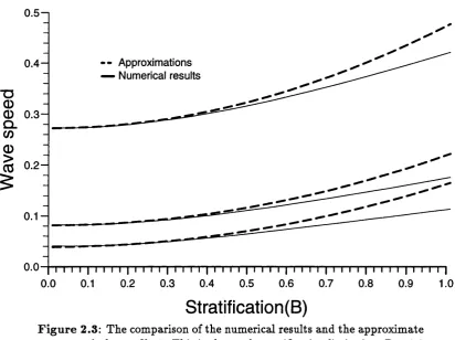
^ J o ( ^ y d z . (2.3.15)

Evaluating (2.3.15) and combining it with (2.3.13) gives (fig.2.3)

C<1) = 0.2724 + 0.2019B^ + 0 ( B %

c<^) = 0.08127 + 0.1382B' +

= 0.03865 + 0.1240B' + 0{B*). (2.3.16)

Higher orders follow similarly.

c. Arbitrary stratification

The strong and weak stratification results can be combined efficiently into an

approximation to the eigenvalue valid for all values of B by introducing the two

point Fade approximation of the form

(30)

0.5-1

- - A pproxim ations — Num erical results

0.4-■D

CD

0) 0.3-

Q . CO

^

:

m 0 2

-0.1

-0.0

0.2 0.3 0.4 0.5 0.6 0.7 0.8

0.0 0.1 0.9 1.0

Stratification(B)

F igure 2.3: The comparison of the numerical results and the approximate wave speeds for profile 1. This is the weak stratification limit, 0 < B < 1.0 accurate to 0{B^). As in the previous figure the asymptotic results are good for surprisingly high values of the expansion parameter

The coefficients a^, /?» are chosen so th at the values for c coincide with the previous

approximation in the limits B 0 , B oo and the orders n, m are chosen to

accord with the number of known derivatives at the limits. Although convergence

is guaranteed at either end, it is by no means sure th at the approximation will

remain finite for all B. P utting in extra coefficients th at cannot be determined

by the number of known derivatives, introduces a degree of arbitrariness which

can be used to ensure there are no zeros in the denominator while still keeping

the same accuracy at either end.

For large B the eigenvalues c increase as B and for small B approach a

constant. In the above example the first three terms are known for both large

and small B, thus consider the approximation

« 0 + oliB -j- 0=2^^ -|- a s B ^ /'o o 1 o \

Expanding this and matching the various terms gives results accurate to 0 {B ^ )

for small B and to 0{B~^) for large B, hence

,(1) 0.2724 -f 0.4687B -f- 0.5477B^ -f 0.40415^

(31)

1.0-1

- - Fade Approximation — Numerical result 0 .9

-'// // // /// /////////////

0.8

0 .7

-"O

0 0.6

-0

Q.

CO g 0 .4

-V777V777777777

0 .3

-0.2

-0.1

-0.0

1.0 1.5

0.0 0.5 2.0 2.5 3.0

Stratification(B)

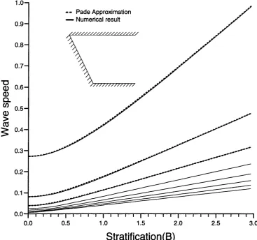
F igure 2.4: The first few numerically computed wave speeds and the Fade approximations for profile 1 for increasing stratification, 0.01-3.0. There is a smooth transition from the barotropic shelf wave modes at small

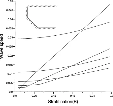
B to the baroclinie IKW modes for large B. The waves speeds are almost linear in B for values of the stratification greater than unity and so all wave modes are essentially IKWs after that point. The Fade approximations are correct to third order at both ends. The relative error is around 1% for the first mode and only slightly more for the next two.

Figure 2.4 shows the first three Fade approximations compared with the num er

ically computed values for a range of B.

The pressure at any point can also be expressed in a Fade approximation.

For small B , p{y,z) = p^^\y) + B ‘^p^^\y^z) -f 0 {B ^ ) and for large B, p{y,z) =

p^^{y, z)-{-B~^p^^{y, z)-\-0{B~^y. The approximation will now depend on y, z as

well as B. Keeping this approximation finite for all y , z and B is more difficult

th an for the phase speed but one solution is to take n and m large enough so

th a t all the (3i are arbitrary and can be chosen appropriately. As the pressure

is completely determined by its value on the shelf, only values there have to be

(32)

Profile 2. Let the stratification be uniform, {N{z) = 1), the surface rigid, (a >> 1) and the shelf have the profile

% ) = (2/ + 1)/2, y < 1 (yr d{z) = - 2 z - 1 , - 1 < z < - 1 /2 . (2.3.20)

The analysis for this profile is similar to th at above so only differences are noted.

For strong stratification, changing to this profile makes no difference to the

0 { B) term but the second order equation for the m th eigensolution,

introduces an 0 (1 ) term of —2/m ^7r^ to the eigenvalues of the odd numbered

modes. The terms proceed similarly but it is noticeable th at the forms

for even and odd modes are quite distinct.

If B is small there are obviously more alterations. Firstly, the boundary

condition at 3/ = 0 is a no net flux condition at the coastal wall, i.e. +

cpy dz = 0 on y = 0. The governing equation for the (j>n{y) changes to

+ Co(î/ + 1)(^^ — F(<^0> ' • • ) ^ n -l, 2/), U-— 0 , 1 , . . . . (2.3.22)

where F is a complicated function similar to the RHS of (2.3.10) and remains

a non-homogeneous Bessel equation of zero order. (In fact all piecewise linear

profiles give a variation of the Bessel equation.) The homogeneous, barotropic

equation has solutions Jo{2y^{y -f 1 ) /c q) and Yo{2^{y -f- 1 ) /c q) , (j>o{y) is a linear

combination of these two functions and cq arises as a solution of a transcendental

equation derived from the two boundary equations. The procedure for higher

orders is the same as previously and ci appears in an analogous way. There are

IKWs existing for small B which are not found by this procedure because they

exist on much smaller scales. Rescaling to consider distances of 0 { B ) from the

coast straightforwardly gives first order solutions. The phase speeds are of course

simply F/2m7T, m = 1 , 2, . . . and the eigenfunctions cos 2m7Tz.

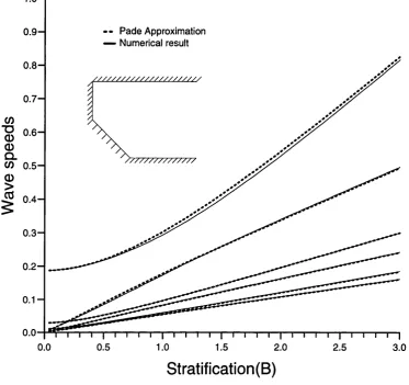
Approximations valid for all B can be obtained by introducing Fade approx

imations as before. Figure 2.5 shows the comparisons between the these and the

(33)

1.0-1

- - Fade Approximation — Numerical result 0 .9

-0.8

0 .7

-"5 0.6

-Q .

CO 0 .5 - 77777777777777

0 .4

0 .3

-0.2

-0.1

-0.0

1.0

0.0 0.5 1.5 2.0 2.5 3.0

Stratification(B)

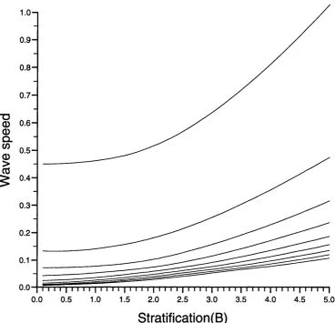
F igure 2.5: The first few numerically computed wave speeds and the Fade approximations for profile 2 for increasing stratification, B, 0.01-3.0. There is no longer a smooth transition from the barotropic shelf wave modes at small B to the baroclinie IKW modes for large B. Hence the Fade approximations cannot fully capture the behaviour of the modes. However away from the “kiss” the accuracy is very good.

§2.4 N u m e ric a l M e th o d

The numerical method presented here relies upon an integral representation

of (2.2.4). This requires th at a Green’s function is found th a t satisfies (2.2.4a)

everywhere except at a point yo,zo. The divergence theorem then gives an ex

pression for p{yo, zq) in terms of an integral along the shelf. The Green’s function,

G (r|ro ), does not have to satisfy the boundary condition on the shelf, only the

conditions on z = 0, z = —1. Rescale 2.2.4 by setting z' = B z and H{y) = Bh{y).

Drop the primes to get

(34)

H'v + c{H'py + = 0, {z = - H { y ) )

or

— cP .n = 0, [z = —H[y)) (2.4.16)

where P = {Py,PzlN^), n is the outward normal vector to the slope and m{y) =

H ' I s/1 + The top boundary condition is now

a^Pz + BN^{0)p = 0, {z = 0) (2.4.2)

For uniform stratification and a rigid lid (a 1) a closed form solution for

(

7

(r|ro) can be found. The function now satisfies Poisson’s equation

= 2TrS{r - fq), (2.4.3)

with no normal derivative on 2; = 0, —B. Use the conformai map w = sinh(7rz/J9)

to transform the infinite strip into the half plane. Find G (r|ro) by using the

m ethod of images to get the fundamental solution

G (r|ro) = log | sinh ^ (3/ - 3/0 + - zo)) sinh ^ (3/ - 3/0 + i{z + zq)) |.

(2.4.4)

This solution behaves like iry jB a.s y 0 0 so subtract Tr(y + V o )I B from

(2.4.4) to get a more appropriate G (r|ro).

If the solution for non-uniform stratification and/or a free surface is required

then G (r|ro) must be found as an infinite series. The z-dependence of the homo

geneous solution of (2.4.1) can be expressed in terms of orthonormal eigenfunc

tions Zn th at satisfy

( iV - '^ ;) ' + A X = 0, (2.4.5a)

Z ; = 0, (z = - B ) (2.4.56)

+ B N \ 0 ) Z „ = 0. (z = 0) (2.4.5c)

Expemd G (r|ro) and the S function as a series of Z„, i.e.

0 = E M y ) Z n ( ^ ) , ^(r - ro) = E % - yo)Z^(zo)Z„(z), (2.4.6)

(35)

where the functions must satisfy the non-homogeneous ordinary differential

equations

~ = 27rZn{zo)8{y - yo), n = 0,1,2 . . . (2.4.7)

Use the m ethod of variation of parameters and the conditions th at each Fn[y)

is bounded as 2/ —► oo and 7^(0) = 0 to get th at

Fn(y) = ra = 0 , 1 , 2 . . . (2.4.8)

and therefore

G (r|ro) = - f ; ^(e-M t/+vo) + (2.4.9)

n = 0

as the analogue to (2.4.4). This has exponentially small behaviour as y —> oc so

long as An ^ 0 for any n, (true for any finite a). The divergence theorem gives

/ [ pC{G} - GC{p} dA = J (pG - G P ).n ds (2.4.10)

A S

where S is the boundary around the domain A and G = {G y , G z /N “^). As

£{p} = 0 in A and C{G} = 0 everywhere except the point (î/o,^o), the LHS

reduces to 'KmPoz where po = vivo^zo) and Tr^ is equal to 27t if the point {yo^zo)

is an interior point. If the point is on the boundary then 'Km corresponds to the

interior angle at the boundary (tt if the gradient is continuous there) or twice

th at angle if the point is on the bottom . This is because the singularity at the

image point coalesces with th at at the source point. In the free surface case, if

the point is on z = 0 the value of will depend non-trivially on the value of

B A (0 )/a .

There is no contribution from the top or bottom boundaries as p and G (r|ro)

satisfy the same boundary conditions there. Also Py —> 0 and Gy —>■ 0 as p ^ oc.

Substitute the boundary condition on C (the shelf) to eliminate P , so th at

J

pGm ds = c

I y

p G .n ds — Tr^iPo

j

. (2.4.11)

This gives the pressure anywhere in the fluid in terms of the pressure on the shelf.

(36)

can in fact be removed to give

J { P ~ Po)Gm ds-^po J Gm ds = c l j { p - po)G .n ds - J di/ > .

c c (c ^ 't o p j

(2.4.12)

The integral along the top is equal to zero in the rigid lid case. If there is a free

surface, consideration of Green’s theorem around the circuit z = 0,y = 0, z =

—b,y —> OO shows th at the integral is 27T, provided th at (yo,^o) is not the origin.

In th at case the integral is found by summation.

As the line integrals are now bounded they can be evaluated using Simpson’s

Rule with N intervals. This will give an equation for po in terms of pi,i = 1, AT+1,

where pi is the value of p at the ith end point r; = (t/^, z*). As dz = —m{y)ds, the

integration can be made with respect to z on [ - B , 0]. Choosing the point {yo, zq)

as each end point successively leaves AT + 1 distinct equations. For j = 1, AT + 1

( / N + i \ N + i \

^ { P j \ ^ E ^ H j \ - h eiPiDij > =

I

V

J

{

N + l ) N + 1

h Y ^iGij — F j \ — h Y (2.4.13)

where Dij = G (r;|rj).n /m (y i), Fi = G (r(z)|ri) dz, Gij = G (r;|rj), Hi = 0

if there is a rigid lid or Hi = 2TT,i > 0 if there is a free surface, e» are the

Simpson’s rule coefficients and h is the step size. The orthogonality condition is

Yjheipl'^^Pi^^ = 0 for distinct n , m . Multiply (2.4.13) by ej to ensure th at the

RHS is symmetric in i and j . This is a complete ATd-1 x AT+1 general eigenvalue

problem A p = cBp, p = (pi,P2, • • • jPiV+i)? where A is a real symmetric m atrix and

B is a real m atrix. The problem of finding the form and speed of low-frequency

coastally-trapped waves has been reduced to a linear eigenvalue problem th at can

be solved using standard algorithms.

For typical oceanic values of a « 10, the modes are not significantly changed

from the rigid lid case. The fundamental external Kelvin wave mode (conven

tionally mode 0), which depends on finite Rossby radius for its existence, is not

present but in any real situation travels much faster than the other modes.

The integral formulation extends to non-zero wavenumbers directly. The gov

erning equation is then Helmholtz’s equation. If z is rescaled in (2.2.1) as in

(37)

exactly the same form as (2.4.9) except that the combination yjk^ — w^)A^

appears everywhere instead of Equation (2.4.11) follows immediately with

the vector G = (Gy, (1 — uj^)Gz/N^)- The singularities can be removed as before

but an extra term now appears on the RHS of (2.4.12). Equation (2.4.13) fol

lows but with the term H j now equal to tt^ — JqG.nds which can be evaluated

numerically.

However the matrices th at result now depend on the values of w and k them

selves. The eigenvalue problem is no longer linear and so a different search pattern

has to be used. Since all the eigenvalues are real, one technique would be to fix

k and find all the zeroes of /(w ) = det[kA — u B ) . This is more time-consuming

than in the low-frequency case but the advantages of increased resolution, di

rectness and one-dimensionality are maintained. This is especially true if some

estim ate of the frequency and wavenumber is known.

To test the model, consider the case where the shelf is vertical. W ith a rigid lid

the eigenvalues are simply B I mr, n = 1 , 2. . . . The numerical results are accurate

to 3 decimal places with 20 intervals along the shelf and to 4 decimal places with

40 intervals. Figures 2.2, 2.3 show the comparison with the expansions drawn

from the results of the previous section and it is clear th at the correspondence is

excellent for B < 0.5 and B~^ < 0.7, the limits of the accuracy of the expansions.

Though not as immediately versatile as the suite of programs developed by

Brink and Chapman, the fact th at analysis has reduced the problem to only one

dimension does allow greater definition and accuracy. It is possible to obtain

all possible eigenvalues for a particular case at the same tim e, an improvement

which allows fuller investigation of modes and their scattering. There is also a

large increase in resolution over the previous methods for an equivalent number of

points. For example, most of the results have been arrived at using 50-60 points

across the shelf, while the Brink and Chapman programs use a fixed 17x25 point

grid which extends to the far field boundary condition. This implies they have at

most 12-13 points across the shelf and so do not resolve any mode higher than

mode 6. Higher modes require extra points which the new m ethod accommodates

much more efficiently.

For a typical problem, this m ethod takes 6.4 seconds of CPU tim e for 3 sig.

The calculation, scattering and stability of topographic rossby waves