Who is behind the wheel? Driver identification and fingerprinting

Who is behind the wheel? Driver

identification and fingerprinting

Saad Ezzini

_{, Ismail Berrada}

_{and Mounir Ghogho}

Introduction

In the era of the Internet of Things (IoT), every object can be made smart with embed-ded sensors, and connected to the internet through wireless technologies. The term “smart” was introduced first for the mobile phone, and the term smartphone was used for the first time in 1999. After 2012, smart watches and other wearable devices became popular. The massive data collected with smart phones and wearable devices offer unprecedented opportunities for human behavior modeling, real-time health monitor-ing, and personalised services.

When people think of IoT, phones, watches, and other small devices often spring to mind. However, automobile manufacturers are now embedding into their vehicles Wi-Fi, global positioning system (GPS) and a bunch of sensors that collect data about the vehi-cle and the driving behavior. Soon, every car will be connected to its manufacturer, to service companies, to insurance carriers, to its drivers, and to the world around it. Gartner predicts that there will be a quarter of a billion connected vehicles by 2020 [1]. Most cars now have over 400 sensors built into them, capturing data every few milli-seconds about steering wheel movement, tire pressure, driver actions, speed, GPS posi-tion, car wear and tear, and more. Autonomous cars generate dozens of operational data

Abstract

In the last decade, significant advances have been made in sensing and communica-tion technologies. Such progress led to a considerable growth in the development and use of intelligent transportation systems. Characterizing driving styles of drivers using in-vehicle sensor data is an interesting research problem and an essential real-world requirement for automotive industries. A good representation of driving features can be extremely valuable for anti-theft, auto insurance, autonomous driving, and many other application scenarios. This paper addresses the problem of driver identification using real driving datasets consisting of measurements taken from in-vehicle sensors. The paper investigates the minimum learning and classification times that are required to achieve a desired identification performance. Further, feature selection is carried out to extract the most relevant features for driver identification. Finally, in addition to driv-ing pattern related features, driver related features (e.g., heart-rate) are shown to further improve the identification performance.

Keywords: Driver fingerprinting, Driver identification, Driver verification, Machine learning

Open Access

© The Author(s) 2018. This article is distributed under the terms of the Creative Commons Attribution 4.0 International License (http://creativecommons.org/licenses/by/4.0/), which permits unrestricted use, distribution, and reproduction in any medium, provided you give appropriate credit to the original author(s) and the source, provide a link to the Creative Commons license, and indicate if changes were made.

RESEARCH

*Correspondence: [email protected] 1 _{FIL, TICLab, International} University of Rabat, Rabat, Morocco

streams (one terabyte per hour). As the number of connected cars increases, the volume of data generated by vehicles will explode. Powerful analytic platforms will enable insur-ance firms, car companies, service and repair shops, and fleet owners to generate break-through insights.

It is now widely accepted that everyone has a unique way of driving. Thus, driver iden-tification can be performed with high accuracy through driving behavior classification based only on raw data collected from in-vehicle sensors via the Controller Area Net-works (CAN) system. This can be achieved after a few minutes only behind the wheel.

The ability to recognize a driver and his/her driving behavior could form the basis of several applications, such as driver authentication for security purposes, detection of the driver’s drowsiness, and customization of the vehicle’s functions to suit the driver’s pre-ferred configuration.

The problem of automatic driver identification has received increased interest in the recent literature. Despite this interest, the issue of the impact of the identification time on performance has been neglected. With this in mind, the aim of this work was to develop a time-optimized driver identification framework.

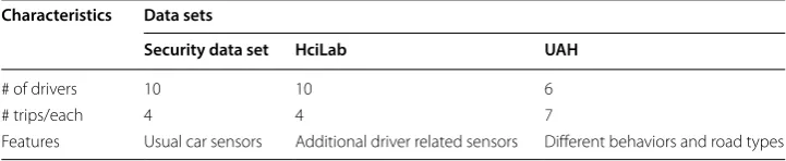
In this paper, we first evaluate the performance of existing driver identification meth-ods using various datasets and explore ways to improve them. Then, we determine the most valuable features for a reliable driver identification. Finally, we look into how to reach a high identification accuracy while optimizing the number of features, the train-ing dataset size, and the identification time (i.e. duration of the testtrain-ing time). The three real datasets used in this paper are summarized in Table 1 [2–4].

The rest of this paper is organized as follows. “Background and related works” section summarizes the existing literature on driver identification and profiling through data analysis. “Methodology and analysis” section describes in details the datasets and the identification methods used in this paper. “Experimental results” section presents the driver identification results and a comparative analysis of the different methods. Finally, concluding remarks, discussions and directions for future work are given in “Discussion” section.

Background and related works

Vehicle-based performance technologies infer driver behavior by monitoring car sys-tems such as lane deviation, steering or speed variability. Such syssys-tems are critical to detect and avoid driver drowsiness, which is related to around 20% of severe car inju-ries. The idea of fingerprinting drivers from timestamped sensor data, e.g., controller area network (CAN) protocol records, is not new; many recent studies have shown that identifying a driver using machine learning-based classification is a promising field

Table 1 Characteristics of the used datasets (more details in the third section) Characteristics Data sets

Security data set HciLab UAH

# of drivers 10 10 6 # trips/each 4 4 7

of research. Another approach to driver identification, which has also attracted a lot of research effort, is based on face recognition. In this paper, we focus on the former approach.

Most methods in the literature on driving style modeling rely on a human-defined driving behavior feature set, which consists of handcrafted vehicle movement features derived from sensor data. These features are used by machine learning methods (super-vised classification, unsuper(super-vised clustering, or reinforcement learning) to solve prob-lems such as driver classification/identification, driver performance assessment, and individual driving style learning.

Both simulated and naturalistic driving patterns have been studied in the literature using different features extracted mainly from the in-vehicle’s CAN Bus (the steering wheel, the vehicle speed, and the engine speed, etc.). The number of these features may range from one to twelve. Using these features, different machine learning methods (e.g. Bayesian algorithms, Decision Tree algorithms, instance-based algorithms, deep learn-ing algorithms) have been proposed to learn drivlearn-ing styles.

approaches to driver identification, for naturalistic data, was proposed by Enev et  al. [15]. Twelve features from the CAN bus were considered with SVM, Random Forest, Naive Bayes, and k-nearest neighbor (KNN) algorithms. The authors have shown that it is possible to differentiate between drivers with 100% accuracy under some assumptions, and it is possible to reach high identification rates using less than 8 min of training time. Recently, Wallace et al. [16] have studied a large dataset of all trips made by 14 drivers over a 2-year period. The authors identified a two-phase relationship between the mean and maximum accelerations within each driver’s acceleration events. This can be used as a measure of a driver’s signature. Burton et al. [17] proposed a novel approach for driver authentication, where the mode of driving is constructed using the following features: pedal control, steering, speed, and distance traveled. The authors used classical machine learning algorithms (SVM, KNN, and Decision Tree) and boosting to increase the clas-sification accuracy. The obtained results show a time-to-detection of 2 min and 20 s at 95% precision.

Methodology and analysis Driver fingerprinting

A higher accuracy of driver identification will likely require multiple driving parameters and a larger learning time. In this paper, we investigate the relationship between accu-racy, the number of features and the learning time with the objective to optimize the driver fingerprinting task.

The process of driver fingerprinting consists of first preprocessing the driving datasets, selecting the most relevant features and then developing appropriate classification mod-els using machine learning algorithms.

Datasets description

There are existing modules (e.g., after-market auto assurance dongles, phone intercon-nected dashboards like Apple’s CarPlay or built-in radios like the telematics unit) that can access a vehicle’s internal computer network and read data for various purposes, including driver fingerprinting.

The three datasets used in this work are described next.

Security dataset [2]

The data collection was carried out in South Korea using a recent model of KIA Motors Corporation. Ten drivers participated in the experiments setting which consists of four paths of three types, city way, motorway and parking space, with a total length of 23 km (Fig. 1). The city way has signal lamps and crosswalks, but the motorway has none. In the parking space, the drivers were required to drive slowly and cautiously. The experi-ment started on 28 July 2015. The time factor was controlled by performing experiexperi-ments in similar time zones from 8 p.m. to 11 p.m. on weekdays. The drivers completed two round trips for a reliable classification. The driving data per driver were labeled from “A” to “J.” A total of 94,401 records every second were captured leading to a 16.7 MB dataset.

For example, ECU monitors and controls the engine, automatic transmission, and Anti-lock Braking System (ABS). ECU measurements are obtained via the OBD-II system. The data are recorded every second during driving. A total of 51 features were measured through the OBD-II system.

UAH‑DriveSet [3]

The UAH-DriveSet is an open dataset obtained by the driving monitoring app “Drive-Safe” with the objective of collecting driving data in different environments using smart-phones sensors alone. The large number of variables included in this dataset facilitates driving analysis.

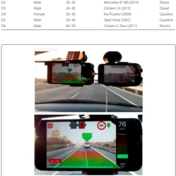
The dataset was collected by six drivers with diverse ages and vehicles, including a fully electric vehicle. Three behaviors (normal, aggressive and drowsy) were performed by each driver in two different routes, one is 25 km long (round trip) on a motorway type of road with usually three lanes in each track and a maximum speed of 120 km/h; the other is around 16 km long on a secondary road of usually one lane in each track and a maximum speed of about 90 km/h. In the case of secondary road, only normal and drowsy behaviors were simulated with the electric car because of issues related to lack of autonomy. The resulting recording amounts to more than 500 min of realistic driving with its associated raw data and supplementary semantic information, together with the video recordings of the tours. Other details about the experiment are given in Table 2.

The tests were performed on the cars of the drivers by placing two phones on their windshield. Figure 2 shows the setup reproduced on each tester.

Every driver drives on pre-designated routes by simulating sequences of different behaviors: normal, aggressive and drowsy driving. In the case of ordinary driving, the driver is told to drive as usual. In the sleepy case, the driver is told to pretend slight sleepiness, which typically results in sporadic unawareness of the road scene. Finally, in the case of dangerous/aggressive driving, the driver is told to drive to the limit his aggressiveness (without putting the driver at risk), which generally results in impatience

and roughness while driving. The co-pilot is in charge of the safety of the tests, and does not interfere by giving any additional instruction during the tours, except in cases of extreme danger during the maneuvers. The two different roads covered in the tests are both in the Community of Madrid (Spain).

The data is composed of two files whose names start with “RAW” and which contain measurements obtained directly by the inertial sensors (gyroscopes and accelerometers) and the GPS of the smartphone. The two files are described below:

(a) Raw GPS contains the data obtained from GPS, at 1  Hz sampling frequency. The content of each column is described below:

• Timestamp (seconds), • Speed (km/h),

Table 2 List of drivers and vehicle that performed the tests (UAH-Driveset)

Driver Genre Age range Vehicle model Fuel type

D1 Male 40–50 Audi Q5 (2014) Diesel D2 Male 20–30 Mercedes B 180 (2013) Diesel D3 Male 20–30 Citröen C4 (2015) Diesel D4 Female 30–40 Kia Picanto (2004) Gasoline D5 Male 30–40 Opel Astra (2007) Gasoline D6 Male 40–50 Citröen C-Zero (2011) Electric

• Latitude coordinates (degrees), • Longitude coordinates (degrees), • Altitude (meters),

• Vertical accuracy (degrees), • Horizontal accuracy (degrees), • Course (degrees),

• DifCourse: course variation (degrees).

(b) Raw accelerometers contains all the data collected from the inertial sensors, at 10 Hz (obtained from the phone’s 100 Hz sampling frequency data by calculating the mean of every ten samples). The iPhone was fixed on the windshield at the start of the route, so the axes are the same during the whole trip. These were aligned in the cali-bration process of DriveSafe, where the y-axis is aligned with the lateral axis of the vehicle (reflects turnings) and z-axis is aligned with the longitudinal axis (positive value reflecting an acceleration, and a negative value reflecting a braking). The accel-erometers measurements were also logged filtered by a Kalman Filter (KF). The con-tent of each column is:

• Timestamp (seconds),

• Boolean of system activated (0 if < 50 km/h), • Acceleration in X (Gs),

• Acceleration in Y (Gs), • Acceleration in Z (Gs),

• Acceleration in X filtered by KF (Gs), • Acceleration in Y filtered by KF (Gs), • Acceleration in Z filtered by KF (Gs), • Roll (degrees),

• Pitch (degrees), • Yaw (degrees).

HciLab dataset [4]

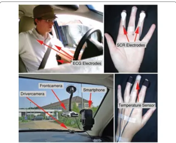
The HciLab Driving dataset is publicly available as an archive of comma separated files where each file contains the merged data set of the recordings of one participant. The complete data set has a size of 450 MB and consists of 2.5 million samples. It is anonymized and contains information about GPS, brightness, acceleration, physiological data, and data of the video rating. Note that the number of samples per participant var-ies due to different traffic conditions and driving behaviors resulting in different driving times. The video is excluded from the data set for privacy reasons.

the road) and a view of the driver. As all data sets were recorded with different sampling frequencies, timestamps were used to synchronize all data post-recording. Details about the different measurements are given next.

The GPS information is recorded at a 1 Hz sampling frequency via the mobile phone. The GPS data consists of the longitude and latitude values (in degree) that define the position of the car, as well as further information about accuracy (in meter), altitude (in meter), speed (in meter per second), and bearing (in degree). A timestamp has been recorded as well to map the GPS data into the rest of the dataset.

The smartphone also provided records of the brightness level (in Lumen) as well as the acceleration perceived by the phone’s sensors along the three axes. These two sensors provide records at frequencies between 8 Hz and 12 Hz.

The electrocardiogram (ECG, in µV) was recorded at 1024 Hz and was used to calcu-late the heart-rate (beats per minute) and heart rate variance at 128 Hz. Furthermore, the skin-conductance (in µS) and body temperature (in degree Celsius) were recorded at 128 Hz. Again, timestamps were added with the physiological data records.

The proposed driver identification model

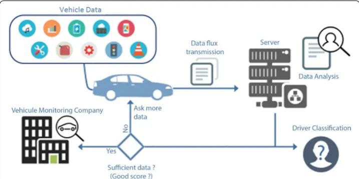
Given the heterogeneity of mobile devices and vehicles, driver identification using in-vehicle sensors needs to adapt its parameters to each context. The optimization of the training time for each context is necessary for reliable and fast driver identification.

Figure 4 describes the process of performing such optimization. In this process, the datasets are first divided into small segments, and classification algorithms are applied on an increasing number of segments until the identification score reaches a pre-defined threshold of satisfaction (ideally 100%). The obtained results are then saved on the server. Figure 5 shows the driver verification framework based on the analysis of driving patterns.

The framework consists of four modules which are data collection, data preprocess-ing, driver classification, and driver verification. Data collection from the in-vehicle sen-sors begins when the driver starts driving. The data preprocessing module converts the collected data into a new format to be analyzed by the next module, and builds feature vectors that can distinguish drivers. The driver classification module trains the machine learning algorithm using the feature set fed from the previous module. The machine learning algorithms considered here are Extra Tree, Random Forest, KNN, and SVM, which were shown to yield high performance in previous studies. The machine learning algorithm detects the unique driving patterns for a driver and builds his or her driv-ing fdriv-ingerprints. The driver verification module compares a given drivdriv-ing pattern with those of the authenticated drivers and decides on whether there is a match or not. More details about data preprocessing and feature analysis are given next.

Fig. 4 The proposed driving pattern learning model

Data preprocessing

The objective of this task is to transform the collected data for the subsequent analysis and classification algorithms. This task consists of the following subtasks.

1. Data preparation and cleaning constant and identical columns are removed. For example, the engine torque value is identical to the correction of engine torque value. After deleting redundant features, we replace the missing values or wrong ones using the KNN method.

2. Feature selection after data preparation, we select the most contributing features and exclude those that are highly correlated with them in order to improve the driver identification performance in terms of accuracy and speed.

3. Feature transformation first, the time is transformed from date-time format to timestamp format in order to easily include this feature in the learning algorithms. Then, the dataset is split into multiple segments to be used in the subsequent opti-mization process. Further, as the features have different scales, they are normalized prior to their use in the machine learning algorithms. Indeed, the normalization process is necessary for algorithms that are based on the distance between data ele-ments, such as the KNN algorithm. This normalization is performed using Eq. (1), where Xi is the normalized version of feature xi; the resulting normalized features lie

between 0 and 1.

For the SVM algorithm, data standardization is also carried out in order to make data dimensionless. After standardization, all knowledge of the scale and the location of the original data may be lost. It is essential to standardize variables in cases where the differ-ence measure, such as the Euclidean distance, is sensitive to the changes in the magni-tudes or scales of the input variables [18].

Feature modeling and analysis

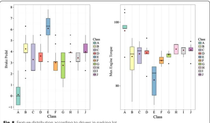
Here, the distributions of the features are explored. Figures 6 and 8 show these distri-butions for two important features: ‘Brake Pedal’ and ‘Max Engine Torque’. The values of these features change with the driving environment such as start-up, idling in heavy traffic, cruising down the highway, etc. [19] and with the driver’s driving pattern in such conditions.

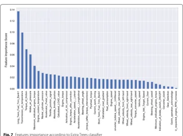
In Fig. 7, the features are sorted according to their ability to differentiate between driv-ers when using the Extra Trees classifier. Top of the importance list are ‘Long-term fuel trims bank1’ which checks the condition of the engine, ‘fuel trims’ which represents the percentage of change in fuel over time. Thus, fuel-related features seem to be the most telling indicators of a driver’s driving style. Transmission oil temperature (a fluid tem-perature inside the transmission) and the ‘Friction torque’, known as ‘brake pedal’, are the next most discriminative features for classifying drivers.

(1) Xi=

xi−min(xi)

Experimental results Classification algorithms

The machine learning algorithms considered in the classification task are Decision Tree, Random Forest, Extra Trees, KNN, SVM, Gradient Boosting, AdaBoost based on Decision Tree, and multi-layer perception (MLP). For the Security dataset, we used the fifteen most important features, according to Fig. 8, along with the normalized times-tamp. For the HciLab dataset, all features were used in the classification task. For the

Fig. 6 Boxplots for two features and for many drivers

UAH-DriveSet dataset, only the GPS-related features were used in the classification, since the sensors have different sampling frequencies and are not synchronized.

Each of the above-mentioned classification algorithms generates a driver identification model.

Evaluation criteria

Since the minimum (over the studied datasets) sampling frequency of driving records is nearly 1 Hz, the driver identification process was performed every minute, so that the number of records per feature in the identification task is at least 60. We adopt a 10-fold cross-validation to compare the different classification algorithms. When a new driving data is fed, the evaluation module classifies it into one of the pre-defined classes.

Identification results

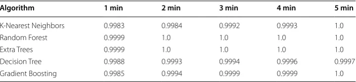
Table 3 shows the classification accuracy for three algorithms during the first 5 min for the security dataset. All algorithms have an accuracy of at least 90%.

As can be seen in Table 3, the rate of increase of the identification accuracy beyond 3 min is very small; this analysis is useful for setting the threshold on the required train-ing time.

Fig. 8 Feature distribution according to drivers in parking lot

Table 3 Identification accuracy for knn, ransom forest and Extra Trees algorithms and dif-ferent training (Learning) times using the security dataset

Algorithm 1 min 2 min 3 min 4 min 5 min

For the second dataset (Hcilab), Table 4 shows the classification accuracy for five algo-rithms during the first 5 min. All algoalgo-rithms achieve the 100% accuracy, which illustrates the positive impact of including physiological features.

For the third dataset (UAH-DriveSet), an accuracy of 76% is achieved using only GPS data.

Model comparison

Driver identification is particularly useful when it is fast. However, faster identification requires a smaller processing window and more reliable identification requires a longer processing window. To strike a good balance between these two constraints, we propose to choose the processing window for each classification algorithm according to the rate of improvement of the classification performance with respect to the processing win-dow. In other words, the identification time (i.e. length of the processing window) is set to the minimum value beyond which the improvement in classification performance is no longer significant. Table 4 shows the classification performance for different algo-rithms and different identification times. It can be shown that Extra Trees and Random Forest algorithms perform better than the other algorithms considered in this work.

Driver verification

Using the classification model trained by authorized users, driver verification consists of testing whether or not the user is classified into one of the pre-defined classes, e.g., authorized drivers. The testing process is based on the computation of the probability of occurrence of each the pre-defined classes given the new data samples. For the Random Forest algorithm, these probabilities are computed using the frequencies of each class, given a new driving pattern, among the large number of generated trees. If all computed probabilities fall below a pre-defined threshold, the driver is declared not to be one of the authorized drivers, and thus an alert may be sent to the owner of the car or the vehi-cle control center. To minimize the probability of false alert, this threshold must be cho-sen judiciously, according to the minimum accuracy obtained in the training phase. In our experiments, the threshold value is set to 0.97.

In our experiment, data related to two drivers of the Security dataset were not included in the training phase and were thus used to test the driver verification task. The maxi-mum of the class probabilities was 0.6 for the first driver and 0.49 for the second driver. As these values are lower than the set threshold, the drivers were successfully identified as non-authorized users.

Table 4 Algorithm accuracy for different algorithms and different training times using the HCILAB dataset

Algorithm 1 min 2 min 3 min 4 min 5 min

Discussion

The proposed approach was successfully applied to three different datasets. In order to further evaluate the merits of this approach, more driving datasets must be tested.

Furthermore, although the proposed driver verification method has been shown to be effective in the case studies presented in this paper, which involve a rather small number of drivers, it is not clear whether this will hold true in the case of a larger number of drivers. Therefore, further studies are required to investigate this issue..

Conclusions

We proposed a time-optimized driver fingerprinting method based on the driving pat-terns. It is shown that in-vehicle network data, such as fuel trim, brake pedal and steer-ing wheel data, are relevant in accurately identifysteer-ing drivers. It is also shown that it is possible to identify drivers with a very high accuracy within the first 3 min of driving, using a limited amount of sensor data collected from a restricted but judiciously chosen set of sensors.

Authors’ contributions

SE and IB discussed the idea of optimizing driver identification and its implementation aspects. SE has implemented the idea and contributed towards the first draft of the paper under the guidance of IB and MG. MG thoroughly proofread the manuscript and made all necessary corrections. All authors read and approved the final manuscript.

Authors’ information

Saad EZZINI has received his Master degree in data science from the Faculty of Science Dhar Mahraz of Sidi Mohamed Ben Abdellah University, Fez, Morocco. Currently, he is pursuing his Ph.D. studies at the International University of Rabat (Morocco). His research interests are in machine learning and its application to intelligent transportation systems and road security.

Mounir GHOGHO has received his Ph.D. degree in 1997 from the National Polytechnic Institute of Toulouse, France. He was an EPSRC Research Fellow at the University of Strathclyde (Scotland) from 1997 to 2001. In 2001, he joined the University of Leeds (England) where he was promoted to full Professor in 2008. He is also currently the Director of TIC Laboratory (TICLab) and a Scientific Advisor to the President at the International University of Rabat (Morocco). He is an IEEE Fellow, a recipient of the 2013 IBM Faculty award, and a recipient of the UK Royal Academy of Engineering Research Fellowship award in 2000.

Ismail BERRADA is a professor at the department of computer science, Faculty of Science Dhar Mahraz, Sidi Mohamed Ben Abdellah University, Fez, Morocco. His areas of interests are in Signal Processing, Networks, and Security. Author details

1 _{FIL, TICLab, International University of Rabat, Rabat, Morocco.} 2 _{Faculty of Science Dhar Mahraz, Sidi Mohamed Ben} Abdellah University, Fez, Morocco.

Acknowledgements

The authors would like to acknowledge the technical support of their colleagues at TICLab and LIMS laboratories. Competing interests

The authors declare that they have no competing interests. Availability of data and materials

All data and content used are open source. The described datasets in “Datasets description” section [2–4] are available at the following links:

1-http://ocslab.hksecurity.net/Datasets/driving-dataset

2-http://robesafe.uah.es/personal/eduardo.romera/uah-driveset/

3-https://www.hcilab.org/research/hcilab-driving-dataset/. Consent for publication

Authors consent the right to publish this paper by Springer Open. Ethics approval and consent to participate

This paper is authors’ own personal research work. Authors self-approve ethical approval and provide consent for participation.

Funding

Publisher’s Note

Springer Nature remains neutral with regard to jurisdictional claims in published maps and institutional affiliations. Received: 19 November 2017 Accepted: 17 February 2018

References

1. Van Der Meulen R, Rivera J. Connected cars will form a major element of the internet of things. 2015. http://www.

gartner.com/newsroom/id/2970017. Accessed 21 Apr 2017.

2. Kwak BI, Woo JY, Kim HK. Driving dataset. PST 2016 http://ocslab.hksecurity.net/Datasets/driving-dataset. 3. Romera E, Arroyo v, BergasaLM. Need data for driving behavior analysis? Presenting the public UAH-DriveSet. In:

Proceedings of IEEE international conference on intelligent transportation systems (ITSC). Rio de Janeiro; 2016. p. 387–92.

4. Schneegass S, Pfleging B, Broy N, Schmidt A, Heinrich F. A data set of real-world driving to assess driver workload. In: Proceeding the 5th international conference on automotive user interfaces and interactive vehicular applications (AutomotiveUI’13); 2013. p. 150–7.

5. Dong W, Li J, Yao R, Li C, Yuan T, Wang L. Characterizing driving styles with deep learning. arXiv preprint

arXiv:1607.03611. 2016.

6. Wakita T, Ozawa K, Miyajima C, Igarashi K, Katunobu I, Takeda K, Itakura F. IEICE “Driver identification using driving behavior signals”. TRANSACTIONS on Information and Systems. 2006;89(3):1188–94.

7. Miyajima C, Nishiwaki Y, Itou K, Takeda K, Ozawa K, Itakura F, Wakita T. Driver modeling based on driving behavior and its evaluation in driver identification. Proc IEEE. 2007;95(2):427–37.

8. Nishiwaki Y, Ozawa K, Itou K, Wakita T, Miyajima C, Takeda K. Driver identification based on spectral analysis of driv-ing behavioral signals. Advances for in-vehicle and mobile systems. Berlin: Sprdriv-inger; 2007. p. 25–34.

9. Meng X, Lee KK, Xu Y. Human driving behavior recognition based on hidden Markov models. In: IEEE international conference on robotics and biomimetics. ROBIO’06. IEEE; 2006. p. 274–9.

10. Choi S, Kim J, Kwak D, Angkititrakul P, Hansen JH. Analysis and classification of driver behavior using in-vehicle can-bus information. In: Biennial workshop on DSP for in-vehicle and mobile systems. 2007. p. 17–19.

11. Wahab A, Quek C, Tan CK, Takeda K. Driving profile modeling and recognition based on soft computing approach. IEEE Trans Neural Netw. 2009;20(4):563–82.

12. Kedar-Dongarkar G, Das M. Driver classification for optimization of energy usage in a vehicle. Proc Comput Sci. 2012;8:388–93.

13. Van Ly M, Trivedi MM, Martin S. Driver classification and driving style recognition using inertial sensors. In: 2013 IEEE intelligent vehicles symposium (IV). IEEE; 2013. p. 1040–5.

14. Zhang X, Zhao X, Rong J. A study of individual characteristics of driving behavior based on hidden Markov model. Sens Trans. 2014;167(3):194.

15. Enev M, Takakuwa A, Koscher K, Kohno T. Automobile driver fingerprinting. Proc Priv Enhanc Technol. 2016;2016(1):34–50.

16. Wallace B, Knoefel F, Marshall S, Porter M, Smith A, Goubran R. Driver unique acceleration behaviours and stability over 2 years. In: Proceedings of IEEE international congress on big data, San Francisco, United States; 2016. p. 230-5. 17 Burton A, Parikh T, Mascarenhas S, Zhang J, Voris J, Artan NS, Li W. Driver Identification and authentication with

active behavior modeling. In: Proceedings of 2016 international workshop on green ICT and smart networking (GISN 2016). Montreal, Canada; 2016.

18 Milligan GW, Cooper. A study of standardization of variables in cluster analysis. J Classif. 1988;5:181. https://doi.

org/10.1007/BF01897163.