DAMAGE QUANTIFICATION RELIABILITY IN BEAMS USING INCOMPLETE
STATIC INFORMATION
Ass. Prof. Dr. Eng. Štimac Grandić I.1, Ass. Prof. Dr. Eng. Grandić D.2 Faculty of Civil Engineering, University of Rijeka, Croatia 1,2
E-mail: [email protected]
Abstract: In the paper a new procedure based on the simple arithmetic operations for location and quantification of damage in beams
using incomplete static information is presented. The grey system theory is employed to locate damage in beam structure using static displacements for two structural stages. Once the location of damage is known, the damage quantification can be done by comparing the displacement curvatures of intact and damage stage of structure. The set of numerical simulations on simply supported beam is conducted to determine the damage quantification reliability of proposed procedure for different damage severities. Also, the results of laboratory test are employed to verify results obtained by numerical simulations.
Keywords: DAMAGE DETECTION, STATIC TEST, DISPLACEMENT, BEAM STRUCTURE
1. Introduction
In the past decades a lot of researches dealt with damage detection, damage localization and damage quantification in different structures such as beams [1,2], plates [3,4], frames or trusses [4]. In general, the damage detection methods can be categorized as: methods based on static structural responses [1,5,6] and methods based on dynamic structural responses [2,4,7]. Also, some researchers combine foregoing structural responses [3]. Some of developed methods can detect and locate the damage [1,8,9] and some of them, beside detection and location, are able to determine the damage severity (quantified the damage) inside the damaged section [2,5,7]. The main problem in both, static and dynamic damage detection methods is incompleteness of structural response information (displacement, mode shape, etc.) i.e. sparseness of measurement [8,9]. Often, algorithms for damage quantification using sparse measurement include solving complicated inverse problems, solving nonlinear optimization problems or using iterative methods [10]. In this paper a new procedure based on the simple arithmetic operations for location and quantification of damage in beams using incomplete (sparse) static displacement is presented. Results of the numerical study and laboratory test are used to determine the damage quantification reliability of proposed procedure for different damage severity.
2. Theoretical formulation of damage detection
and quantification method
Damages in the structures may cause a degradation of structural properties which manifest itself as a change in static responses of a structure. It can be concluded that if there is damage present in the structure its static response will not be the same as the response of an intact structure.
In bent beams, where influence of transversal force on curvature may be neglected, the relationship between curvature, bending moment and bending stiffness can be written as:
) (
) ( ) (
x EI
x M x =
κ (1)
) (
) ( ) (
x EI
x M
x d
d
d =
κ . (2)
where M(x), EI(x), κ(x), Md(x), EId (x), κd (x) are bending moment, bending stiffness and curvature for intact and damaged state of structure. In statically determinate beam, where bending moment is not dependent of the bending stiffness, M(x)=Md(x), equating the equations (1) and (2) gives relationship between bending stiffness and curvatures for two stages of the structure:
) (
) ( ) (
) (
x x x
EI x EI
d d
κ κ
= . (3)
If damage is defined as EId=(1-δ)EI , the decrease in bending stiffness δ can be express as:
) (
) ( 1 ) (
x x x
d κ
κ
δ = − (4)
The curvature of a geometrically and materially linear intact and damaged beams can be written as:
2 2
) ( ) (
dx x w d x =
κ ;
2 2
) ( )
(
dx x w d x
d
d =
κ (5)
where w(x) and wd(x) are displacement lines of intact and damaged structure, respectively.
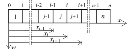
Due to limited number of measurement equipment, only a limited number of displacements can be measured on the structure, i.e. structure may be treated as it is divided in limited number of segments j between measured displacements in positions i=1 to n (Figure 1).
x
i-2 i-1 i i+1
j-1 j j+1
x
i-1x
ix
i+11
n
n-1 n
0 1
w
Fig. 1 The beam's segments “j” and measuring positions “i”
The decrease in bending stiffness δj inside the segment j, can be
now rewritten as:
j d
j j
κ κ
δ =1− (6)
where κj and κjd are intact and damaged curvature of the segment j.
Unfortunately, κj and κjd cannot be calculated directly from known
discrete values of displacement.
The curvature of discrete values of displacement can be calculated at the point xi using next equation:
)
(
)
(
)
(
)
(
2
)
(
)
(
1 1
1 1
i i i i
i i i
i
x
x
x
x
x
w
x
w
x
w
x
−
⋅
−
+
⋅
−
≈
+ −
+ −
κ
(7)where w(xi) is the value of displacement at the point xi, w(xi-1)and
w(xi+1) are the values of displacement at the points xi-1 and xi+1,
respectively.
Similar equation can be written for displacement curvature of damaged structureκd(xi) using values wd(xi), wd(xi-1)and wd(xi+1).
As it can be seen form Eq. (7), the curvatures κ(xi) and κd (xi), at
the position xi (i=1 to n-1) are calculated taken into account the
values of displacement in positions xi-1, xi, xi+1. Bearing that fact in
mind the curvature at the position xi can be treated as average
curvature
κ
at the adjacent segments j and j+1) ( )
( 1
) (
i x i
x j
j i
x =κ =κ +
κ (8)
) ( )
( 1
) (
i x i
x j
d j d i d
x =κ =κ +
κ . (9)
Then
) ( )
( 1
) (
) ( 1 ) (
i x i
x j
j i d
i i
x x
x = − =δ =δ +
κ κ
δ . (10)
Measured or calculated values of displacements usually contained some errors due to different causes, thus, theoretical assumption of zero curvature difference in intact segments will not be fulfilled. Hence, the grey relation coefficient ζ(xi) is employed to
detect the position of significant changes in curvature associated with the damage position [1, 10]
R x
R
R R
x i i
max 5 . 0 ) (
max 5 . 0 min ) (
⋅ +
⋅ + =
ζ (11)
where R(xi) =κ(xi)-κ d
(xi).
In the points where ζ(xi)≥0.6 it will be assumed that there is no
significant changes in curvatures, i.e. δ(xi)=0 [1,10].
Suppose the damage is situated within a single segment j. The grey relation coefficients at the point xi-1 and xi, which are situated
at the beginning and at the end of the damaged segment j, will be less than 0.6, i.e. δ(xi-1)≠0 and δ(xi) ≠0. According to Eq. (10)
calculated vales δ(xi-1) and δ(xi) shows the average value of
decrease in bending stiffness in segments j-1 to j and j to j+1, respectively. As we know that there are no damages in segments j-1 and j+1 the decrease of bending stiffness in segments j=2 to n-1 can be calculated as follows:
) ( ) ( 2
) ( 2 ) ( 2
1 1
i i
i
j x x
x
x δ δ δ
δ
δ = ⋅ − + ⋅ = − + (12)
Determination of decrease of bending stiffness in edge elements (j=1 and j=n) can be obtained by using following equations
) (
2 1
1 δ x
δ = ⋅ (13)
) ( 2⋅ −1
= n
n δ x
δ (14)
because the curvatures in the points i=0 and i=n cannot be determined according to Eq. (7).
Based on the previous considerations, the following damage quantification algorithm is proposed:
a) define κ(xi) and κd (xi)
b) R(xi) =κ(xi)-κ d
(xi).
c)
R R
R R
xi
max 5 , 0
max 5 , 0 min ) (
⋅ +
⋅ + = ζ
d) if ζ(xi)≥0,6 then δ(xi)=0
e) if ζ(xi)<0,6 then
) (
) ( 1 ) (
i d
i i
x x x
κ κ
δ = −
f)
) ( )
( 1
) (
i x i
x j
j i
x =δ =δ + δ
g) if 0
) 1 (
1x =
δ then δ1=0
h) if 0
) 1 (
1 x ≠
δ and 0
) 2 (
2 x =
δ then
) 1 (
1 1 2 δ x
δ = ⋅
i) if 0
) 1 (xn− =
n
δ then δn=0
j) if 0
) 1 (xn− ≠
n
δ and 0
) 2 (
1 − =
− n x
n
δ then
) 1 (
1 2
−
⋅ =
n x
n δ
δ
k) if 0
) (
= i x j
δ or 0
) 1 (
=
−
i x j
δ then δj=0, when i=2 to n-1
l) if 0
) (
≠ i x j
δ and 0
) 1 (
≠
−
i x j
δ then δj =δ(xi−1)+δ(xi), when
i=2 to n-1
m) print δj.
3. Numerical examples
The analysis has been carried out for simply supported beam with different damage severities inside the damaged section of the beam. The span length of the beam is L=9.955 m. The cross section area of the beam is A=2.19⋅10-3 m2, the moment of inertia of intact beam is I=3.83⋅10-6 m4 and Young's modulus is E=2.1⋅108 kN/m2. The applied force at 4.252 m from the left support is F=0.484 kN.
1 2 3 4 5 6 7 8 9 10 11
L=11⋅0.905=9.955 m
F=0.484 kN
0 1 2 3 4 5 6 7 8 9 10 11
Fig. 2 The beam model
The beam is modelled using beam finite elements with knots at both ends of the element (Figure 2). The model has 11 finite elements (1-11) of 0.905 m length and 12 knots (0-11). The displacement have been computed at every finite element knot for both the intact and the damaged state. The bending stiffness of damaged section is reduced by reducing the moment of inertia of intact section for 9 damage scenarios: DS1=10%, DS2=20%, DS3=30%, DS4=40%, DS5=50%, DS6=60%, DS7=70%, DS8=80% and DS9=90%.
3.1 Example 1
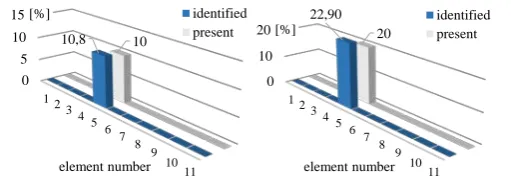
The damage has been simulated by reducing the bending stiffness of the whole 5th finite element (at the distance of 3.62 m to 4.525 m from the left support) as it can be seen in Figure 3. According to the proposed algorithm in Chapter 2 the values of decrease of bending stiffness for each finite element are calculated.
1 2 3 4 5 6 7 8 9 10 11 damaged
section
3.62 m 4.525 m
Fig. 3 The position of damage (example 1)
Comparison of identified (calculated) and present (simulated) damage for all damage scenarios can be seen in Figures 3-7.
0 5 10 15
1 23 4
5 6
7 8
9 10
11
10,8 10
[%]
element number
identified present
0 10 20
1 2 34
5 6
7 8
9 10
11
22,90 20 [%]
element number
identified present
0 10 20 30 40
1 2 34
5 6
7 8
9 10
11
36,30 30 [%]
element number
identified present
0 20 40 60
1 2 34
5 6
7 8
9 10
11
51,30 40 [%]
element number
identified present
Fig. 4 Damage quantification for DS3 (left) and DS4 (right) – example 1
0 20 40 60
1 2 34
5 6
7 8
9 10
11
69,10
50 [%]
element number
identified present
0 30 60 90
1 2 34
5 6
7 8
9 10
11
87,50
60 [%]
element number
identified present
Fig. 5 Damage quantification for DS5 (left) and DS6 (right) – example 1
0 30 60 90 120
1 2 34
5 6
7 8
9 10
11
109,50
70 [%]
element number
identified present
0 50 100 150
1 23 4
5 6
7 8
9 10
11
135,40
80 [%]
element number
identified present
Fig. 6 Damage quantification for DS7 (left) and DS8 (right) – example 1
0 50 100 150
1 2 34
5 6
7 8
9 10
11
164,80
90 [%]
element number
identified present
Fig. 7 Damage quantification for DS9 – example 1
3.2 Example 2
The damage has been simulated by reducing the bending stiffness of a 1/2 of 5th finite element (at the distance of 3.846 m to 4.298 m from the left support) as it can be seen in Figure 8.
1 2 3 4 5 6 7 8 9 10 11 damaged
section
3.846 m 4.298 m
Fig. 8 The position of damage (example 2)
According to proposed algorithm in Chapter 2 the values of decrease of bending stiffness for each finite element are calculated. In Figures 9 to 13, the comparison of identified and present damage for all damage scenarios is presented. Present values of damage are expressed as the mean values of damage in the whole 5th element (i.e. for DS1 the mean value of damage in the whole element is 5%).
0 5 10
1 2 34
5 6
7 8
9 10
11
5,6 5 [%]
element number
identified present
0 5 10 15
1 23 45
6 7
8 9
10 11
12,1 10 [%]
element number
identified present
Fig. 9 Damage quantification for DS1 (left) and DS2 (right) – example 2
0 10 20
1 23 4
5 6
7 8
9 10
11
20
15 [%]
element number
identified present
0 10 20 30
1 2 34
5 6
7 8
9 10
11
29,5 20 [%]
element number
identified present
Fig. 10 Damage quantification for DS3 (left) and DS4 (right) – example 2
0 25 50
1 2 34
5 6
7 8
9 10
11
41
25 [%]
element number
identified present
0 30 60
1 23 4
5 6
7 8
9 10
11
56
30 [%]
element number
identified present
Fig. 11 Damage quantification for DS5 (left) and DS6 (right) –
example 2
0 40 80
1 23 45
6 7
8 9
10 11
75,4
35 [%]
element number
identified present
0 40 80 120
1 2 34
5 6
7 8
9 10
11
102
40 [%]
element number
identified present
Fig. 12 Damage quantification for DS7 (left) and DS8 (right) – example 2
0 50 100 150
1 2 34
5 6
7 8
9 10
11
140
45 [%]
element number
identified present
Fig. 13 Damage quantification for DS9 – example 2
3.2 Example 3
The damage has been simulated by reducing the bending stiffness of a 1/3 of 5th finite element (at the distance of 3.922 m to 4.223 m from the left support) as it can be seen in Figure 14. According to proposed algorithm in Chapter 2 the values of decrease of bending stiffness for each finite element are calculated.
5th element (i.e. for DS3 the mean value of damage in the whole element is 10%).
1 2 3 4 5 6 7 8 9 10 11 damaged
section
3.922 m 4.223 m
Fig. 14 The position of damage (example 3)
0 2,5 5
1 23 45
6 7 8
9 10
11
3,60 3,33 [%]
element number
identified present
0 5 10
1 23 45
6 7 8
9 10
11
8,30
6,67 [%]
element number
identified present
Fig. 15 Damage quantification for DS1 (left) and DS2 (right) – example 3
0 5 10 15
1 23 45
6 7
8 9
10 11
13,80
10 [%]
element number
identified present
0 10 20
1 23 45
6 7 8
9 10
11
20,00
13,33 [%]
element number
identified present
Fig. 16 Damage quantification for DS3 (left) and DS4 (right) – example 3
0 10 20 30
1 2 34
5 6
7 8
9 10
11
29,50
16,67 [%]
element number
identified present
0 25 50
1 23 45
6 7
8 9
10 11
41,20
20 [%]
element number
identified present
Fig. 17 Damage quantification for DS5 (left) and DS6 (right) –
example 3
0 30 60
1 23 4
5 6
7 8
9 10
11
57,60
23,33 [%]
element number
identified present
0 50 100
1 2 34
5 6
7 8
9 10
11
81,80
26,67 [%]
element number
identified present
Fig. 18 Damage quantification for DS7 (left) and DS8 (right) – example 9
0 40 80 120
1 23 45
6 7
8 9
10 11
121,80
30 [%]
element number
identified present
Fig. 19 Damage quantification for DS9 – example 3
4. Test examples
Experimental validation is done by using results of measured deflection on simply supported intact and damaged beam presented in paper [8]. The properties of the test intact beam are the same as those of the numerical example described in Chapter 3. The deflections due to force F=0.484 kN acting at 4.252 m from the left support were measured at every 0.905 m from the supports (at positions N2-N11 in Figure 20).
The damage was introduced by subsequently grinding cuts inside the 5th segment as it is shown in figures 20, 21 and 22 [8]. The decrease in bending stiffness in damaged cross section is about 60% in comparison to intact cross section in both test damage scenarios.
Fig. 20 Test beam specimen [8]
Fig. 21 Test damage scenario 1 [8]
Fig. 22 Test damage scenario 2 [8]
The identified values of decrease of bending stiffness calculated using the proposed algorithm and real decrease of bending stiffness are shown in Figure 22 for test damage scenario 1 and 2 (TDS1 and TDS2), respectively.
0 30 60 90
1 2 3 4
5 6
7 8
9 10
11 68,6
36 [%]
element number
identified real
Fig. 23Damage quantification for TDS1 (left) and TDS2 (right) – test example
0 30 60 90
1 23 4
5 6
7 8
9 10
11 87
60 [%]
element number
identified real
The real value of decrease in bending stiffness due to grinding cuts of 60% of intact bending stiffness at the 60% of segment of 0.905 m for TDS1 is expressed as the mean value of damage to the whole segment.
5. Discussion and conclusion
As it can be seen form conducted numerical and test examples the damage is successfully located in all cases.
The comparison of identified and present/real values of decrease in bending stiffness are shown in Tables 1 and 2 as deviation of identified values to present/real values of decrease in bending stiffness.
As it can be seen from Chapter 3 and Table 1, all identified values in numerical examples are greater than present/real values of decrease in bending stiffness. Generally, proposed method give overestimated values of damage severity. In Chapter 3.1, in case of damage scenarios DS7-DS9, as well as in Chapter 3.3 in case of DS9, identified decrease in bending stiffness is greater than 100% what is fiscally impossible. This phenomena is a result of using algorithm based on simple arithmetic operation and insufficient number of structural response data.
Tab. 1 Deviation of identified and present values of decrease in bending stiffness for numerical examples [%]
Damage scenario Example 1 Example 2 Example 3
DS1 8 12 9
DS2 15 21 24
DS3 21 34 38
DS4 28 48 56
DS5 38 64 77
DS6 46 87 106
DS7 56 115 147
DS8 69 153 206
DS9 83 211 306
In cases where a present damage is the smallest (10%) the deviation of identified over present damage is approximately 10%. In cases of the greatest damage severity of 90% the deviation of identified over present damage is between 83 and 306%. If we compare the same damage scenario it can be seen that overestimation of damage is greater in case where damage is situated on the smallest section, i.e. overestimation of damage is greater if sparseness of data is greater.
Tab. 2 Deviation of identified and real values of decrease in bending stiffness for test examples [%]
Damage scenario Test Examples
TDS1 96
TDS2 45
The results of using test data confirm numerical conclusion. Test damage scenario 1 (TDS1), where damage covers approximately 60% of length of 5th segment can be compared with
damage scenario 6 in numerical example 2 (DS6-2) while test damage scenario 2 (TDS2), where damage covers approximately the whole 5th element can be compared with damage scenario 6 in numerical example 1 (DS6-1). The deviation of identified and present/real values of decrease in bending stiffness for TDS1 is 96% and for DS6-2 is 87%. The deviation of identified and present/real values of decrease in bending stiffness for TDS2 is 45% and for DS6-1 is 46%.
If we suppose that overestimation up to 50% of identified over present/real damage is acceptable in engineering purposes it can be concluded that presented method can be successfully used in detection and quantification of those damages where decrease of bending stiffness is not greater than 40%.
Acknowledgement
This work has been partially supported by University of Rijeka through grant No. 13.05.1.1.01.
6. References
[1] Abdo M. A-B., Parametric study of using only static response in structural damage detection, Engineering Structures, 34, p. 124– 131, 2012
[2] Choi F.C., Li J., Samali B., Crews K., Application of the modified damage index method to timber beams, Engineering structures, 30(4), p. 1124-1145, 2008
[3] Yam L.H., Li Y.Y., Wong W.O., Sensitivity studies of parameters for damage detection of plate-like structures using static and dynamic approaches, Engineering Structures, 24(11), p. 1465-1475, 2002.
[4] Qiao P., Lu K., Lestari W., Wang J., Curvature mode shape-based damage detection in composite laminated plates, Composite structures, 80(3), p. 409-428, 2007.
[5] Yang Q.W.; Sun B.X., Structural damage localization and quantification using static test data, Structural Health Monitoring, 10(4), p. 381-389, 2011.
[6] Štimac I., Uporaba utjecajnih linija progiba u otkrivanju oštećenja konstrukcija, Disertacija, Split, 137 p. 2006. (in Croatian) [7] Zou Y., Tong L., Steven G.P., Vibration-based model-dependent damage (delamination) identification and health monitoring for composite structures—a review, Journal of Sound and Vibration, 230(2), p. 357–378, 2000.
[8] Choi I.-Y., Lee J. S., Choi S., Cho H.-N., Development of elastic damage load theorem for damage detection in statically determinate beam, Computer and Structures, 82(29-30), p. 2483-2492, 2004.
[9] Guan H., Karbhari V.M., Improved damage detection method based on element Strain damage Index using sparse measurement, Journal of Sound and Vibration, 309(3-5), p. 465-494, 2008.
[10] Chen X-Z., Zhu H-P., Chen C-Y., Structural damage identification using test static data based on grey system theory, Journal of Zhejiang University SCIENCE (JZUS), 6A(8) p. 790– 796, 2005.