http://www.sciencepublishinggroup.com/j/ajmie doi: 10.11648/j.ajmie.20190401.12
ISSN: 2575-6079 (Print); ISSN: 2575-6060 (Online)
Copula Estimation Method of the Running Accuracy of Ball
Bearing
Li Lihong
1, 2, Li Jishun
2, Xue Yujun
2, Yu Tongshuai
1, Yu Yongjian
2 1Vehicel & Transportation Engineering Institute, Henan University of Science and Technology, Luoyang, China 2Henan Key Lab for Machinery Design and Transmission System, Luoyang, China
Email address:
To cite this article:
Li Lihong, Li Jishun, Xue Yujun, Yu Tongshuai, Yu Yongjian. Copula Estimation Method of the Running Accuracy of Ball Bearing. American Journal of Mechanical and Industrial Engineering. Vol. 4, No. 1, 2019, pp. 11-20. doi: 10.11648/j.ajmie.20190401.12
Received: January 22, 2019; Accepted: February 28, 2019; Published: May 11, 2019
Abstract:
The bearing is an assembly consisting of multiple elements and its performance is shown mainly as its running accuracy which is influenced by many factors including its elements’ geometrical precision. The influence of elements geometrical precision on bearing running accuracy is joint effect when multiple elements are assembled together. So there must be dependent relationships between bearing running accuracy and the joint action of multiple elements. Such relationship was very complicated and difficultly described by mathematical formula. But, the elements’ geometrical precision follow statistics law, and so, statistics can be applied to analyzing elements’ dimension distribution law and construct joint distribution function. The copula function can be introduced to establish the transmit relationships that join the running accuracy to multiple elements geometrical precision. Based on the copula estimation of distribution algorithm, the mathematic modeling of the radial and face run out distribution of the bearing and elements dimension precision distribution can be built to forecast bearings running accuracy.Keywords:
Bearings, Running Accuracy, Copula Function, Dimension Precision1. Introduction
Ball bearings can be considered as the system consisting of inner ring, outer ring, cage and rolling elements which have themselves geometrical precision. The geometrical precision of these elements can produce very large influence on the running accuracy of the bearing. But few studies about the relationship between them have been reported. In general, the running accuracy of bearings can be estimated by measuring the radical run out and the face run out of finished bearings after assembly and very difficultly gained before assembly. After the elements of bearing were assembled together, they must influence on each other and on the running accuracy of bearings at last. So, there must be the connection between the geometrical precision of elements and the running accuracy of the bearing, but this connection can be difficultly expressed by mathematical formula. However, the geometrical precisions of elements and the running accuracy of bearing follow the regularities of distribution which can be obtained with statistical analysis. The delivered and mapped relation
between the joint distribution of the running accuracy and the multivariate distribution of the element geometrical precision can be constructed by Copula function. So, before assembly the finished bearings can be estimated by element geometrical precision.
to distribution estimation with less operation and can preferably expressed distribution situation of dominant group [17]. With copula function, statistics method can be adopted to analyzing the distribution feature of elements geometrical precision of bearings and the dependence relation between the running accuracy of bearings and multivariate distribution of elements. So, the running accuracy of bearings can be estimated by constructing the mathematic model between the running accuracy and elements geometrical precision before assembly.
2. Copula Theory
2.1. Copula Function
Copula function, also called connective function or dependent function, can connect the joint distribution function of multivariant with marginal distribution function and can also distinguish dependent structure from marginal feature in multivariant distribution. These ideas came from Sklar theorem: the joint distribution function can be decomposed into multiple marginal distribution function and one joint Copula function which join multiple marginal distributions to analyze dependence among variables [18, 19].
2.2. Confirming Copula Function
Copula function need two steps to join the joint distribution function of multivariate to marginal distribution function [20]:
2.2.1. Joint Distribution Function
Set F1(x1), F2(x2), F3(x3),…, Fn(xn) as continuous marginal distribution function, which joint distribution function was set as H(x1,x2,…,xn). These exists a Copula function being written as followed as:
1 1 2 2 3 3 n n
1 2 n
C ( F (x ), F (x ), F (x ),? , F (x ))
= H ( , x , ? , xx ) (1)
Set W1= F1(x1), W2= F2(x2),…, Wn=Fn(xn), the equation (1) can be written as:
1 2
1 1 1
1 1 2 2
(W , ,..., )
( ( ), ( ),..., ( ))
n
n n
C W W
H F− W F− W F− W
= (2)
2.2.2. Copula Function
From the definition of Copula function, many functions can be set as Copula function; two most studied functions were elliptic Copula function and Archimedean Copula function. The most obvious feature of elliptic Copula is that its variables have the same type distribution. The most type of elliptic Copula which was commonly used is multivariate Gaussian Copula (MVN) and multivariate student's Copula (MVT) [21].
Multivariate Gaussian Copula function and its density
function can be expressed as followed:
1 2
1 1 1
ρ 1 2 N
( , ,..., ; ρ)
Φ (Φ (u ), Φ (u ),..., Φ (u ))
N
C u u u
− − −
= (3)
1 2
1/ 2 1
( , ,..., ; )
| ρ | exp( 1 / 2 ς (ρ I) ς)
N
c u u u ρ
− ′ −
= − − (4)
where:
ς
=(ς ς
1, 2,...,ς
N)′, 1( )n un
ς
= Φ− ,n=1, 2, 3, ..., N, ρ is symmetrical positive matrix which elements in the diagonal line are 1, |ρ| is determinant value of corresponding matrix. Φρ(·) expresses multivariate standard normal distribution function, Φ−(1 u)is the verse function of
( )u
Φ , I is the unit matrix.
Copula functions have much superiority in constructing joint distribution function of random variable as followed:
1) Copula theory doesn’t limit selecting marginal function type and can construct flexibly joint distribution by Copula function;
2) when construct mathematical model with Copula function, marginal distribution reports just individual information of univariant, while the information between variables can be shown by Copula function. So marginal distribution of variables and correlativity among them can be studied dividually [22].
3. The Running Accuracy of Bearings
3.1. The Summary of Running Accuracy
To insure running accuracy of transmission parts, antifriction bearing need controlling the radial run out and face run out of bearings in a certain range. The running accuracy of bearings relates to radial run out of inner-outer rings, the face run out of inner-outer ring to raceway, the run out of the benchmark face of inner ring to inner diameter, the tilt chance of prime line in outer ring to benchmark face in which the radial run outs and the face run out of bearings are the important indexes [23].
3.2. Influencing Factors on Running Accuracy
4. Mathematic Modeling
4.1. The Stochastic Variables
Before assembling, the bearing components are independent in geometry accuracy distribution and have self-correlation. But, after assembling, they will influence on and interact with each other. Because of accidental factors in machining, the dimension precision of the inner ring, outer ring and roller has certain randomness and then assembling them is also a stochastic process. So the running accuracy of the finished bearing must be influenced by the geometrical precision of all elements.
Take the deep groove ball bearing for example, the radial run out of bearing and the face run out of bearing to raceway are the important indexes influencing on the running accuracy of bearing. In this paper, without regard for the influence of the cage and other factors, only the inner ring, outer ring and rollers were applied to analyzing the running accuracy of bearing. The influence of the dimension of the raceway in inner ring, the dimension of the raceway in outer ring and the roller dimension on the precision of bearing is the combined efforts. We can
analyze the dimension precision of inner-outer raceway and rollers to estimate the radial run outs and face run out of bearing and then to know the running accuracy of bearing.
Set the radial run-out and face run out of bearing as variables Wt, Dt respectively. For raceway dimension of inner-outer ring, set the upper deviation of raceway in outer ring as xeand the lower deviation of raceway in inner ring as xi respectively. The influence of the roller on bearing precision is a group effect and uniformity of all rollers. The absolute value of the difference between the biggest and smallest dimension of rollers assembled to the bearing is set as random variable xr.
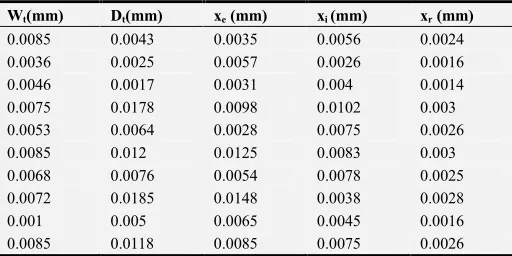
Take 100 groups bearing elements to be numbered and measured respectively and gain 100 groups data about xe, xi, xr. After this 100 groups being assembled, the radial run outs of bearings and the face run outs of bearings were measured in the measuring device and get 100 groups data about Wt, Dt. Due to limitations on space, only the first 10 groups data measured of Wt, Dt, xe , xi , xr list in table 1. Considering that the measuring equipment has error itself, the data in table 1 had been processed by error separation. The following analysis will come from 100 group data.
Table 1. The first 10 groups’ data measured.
No. Wt (mm) Dt (mm) xe(mm) xi (mm) xr (mm)
1 0.0085 0.0043 0.0035 0.0056 0.0024
2 0.0036 0.0025 0.0057 0.0026 0.0016
3 0.0046 0.0017 0.0031 0.004 0.0014
4 0.0075 0.0178 0.0098 0.0102 0.0029
5 0.0053 0.0064 0.0028 0.0075 0.0026
6 0.0085 0.012 0.0048 0.0083 0.003
7 0.0068 0.0076 0.0054 0.0078 0.0025
8 0.0072 0.0185 0.0148 0.0038 0.0034
9 0.001 0.005 0.0065 0.0045 0.0012
10 0.0112 0.0094 0.0078 0.0092 0.0022
4.2. Data Statistical Analysis
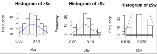
4.2.1. Estimating and Verifying of Variables Distribution For searching for the factors influencing on the radial run-out and the face run out of bearings, the dimension distribution of bearing elements need to be analyzed. The distribution histogram and kernel density estimation of the upper deviation of the raceway diameter in outer ring, the lower deviation of the raceway diameter in inner ring and largest- smallest difference absolute of rollers are shown in Figure 1. The histogram and kernel density estimation of the radial run-out and the face run out of bearings are shown in Figure 2. Form Figure 1 and Figure 2, each stochastic variable
distribution approximately followed normal distribution, but it was only the hypothesis, their normal distributions need to be tested and verified. The results were shown in table 2. In table 2, µ is mean value, σ is variance,
µ
ˆ, ˆσare the estimated value of mean value and variance respectively, P is probability of statistics. In normal condition, if P>0.05, the hypothesis is true, or else, P<=0.05, false.From the table 2, the above hypothesis about the upper deviation of the raceway diameter in outer ring, the lower deviation of the raceway diameter in inner ring, largest- smallest difference absolute of rollers, the radial run out of outer ring and the face run out can’t be refused.
Table 2. Parameters estimated value and verified result of hypothesis.
variables parameters estimated value verified result of hypothesis
µ σ µµµµˆ σσσσˆ p p >0.05
xe 8.035 3.655862 8.035 3.637 0.3896 acceptance
xi 6.813 3.266811 6.813 3.250436 0.459 acceptance
xr 2.346 0.5838604 2.346 0.5809337 0.4327 acceptance
Wt 9.286 4.647852 9.286 4.721862 0.1942 acceptance
Dt 6.394 2.962191 6.394 2.962191 0.1428 acceptance
Figure 2. The histogram and kernel density estimation of Wt(mm), Dt(mm).
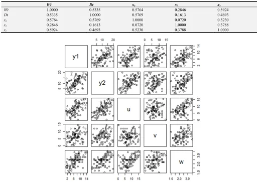
4.2.2. Analyzing Relativity Between Stochastic Variables The covariance matrix between variables in table 1 is shown in table 3. It can be seen that there are very strong relativity between the radial run out, face run out of bearing and the dimension of raceway in outer ring, the dimension of
raceway in inner ring and the dimension difference of rollers. Because of error in dimension, the bearing running must cause the run out of the outer ring. The bigger the error, the more serious the run out. In addition, from the table 3, the raceway in inner ring has stronger relativity with the radial run out than that in outer ring. Before assembly, the raceway in outer ring, the raceway in inner ring and rollers are independent of each other but after assembly , they relate with each other and influence on the whole performance of bearing. The relation chart between xe , xi , x rand Wt , Dt can also be seen in Figure 3. From Figure 3, Wt , Dt have relation to xi , xe , especially, stronger relation to xr that illustrate the running accuracy of bearing bears very stronger relation to the dimension uniformity of rollers. In the precision range, the smaller the difference, the more uniform and the less the run out.
Table 3. The covariance matrix between variables.
Wt Dt xe xi xr
Wt 1.0000 0.5335 0.5764 0.2846 0.5924
Dt 0.5335 1.0000 0.5769 0.1613 0.4693
xe 0.5764 0.5769 1.0000 0.0720 0.5230
xi 0.2846 0.1613 0.0720 1.0000 0.3788
xr 0.5924 0.4693 0.5230 0.3788 1.0000
4.3. Constructing Mathematic Modeling
4.3.1. Mathematic Modeling
After the bearing being assembled, the influence of the dimensional precision of the inner-outer raceway and roller on the bearing running accuracy is the joint effect which can be described very difficultly with ordinary mathematics method. According to Sklar theory, copula function can construct a joint multivariate distribution function with one-dimensional distribution function. So the copula function can be introduced to construct a modeling to estimate the radial run-out of the bearing with multiple one-dimensional marginal distribution function. For being easy to write , the random variables xe , xi ,
xr and Wt, Dt can be replaced by u、v、w and y1 、y2respectively. Their distribution functions are F(u), F(v), F(w), F(y1), F(y2) respectively.
From the above section 3.2.1, u、v、w satisfy the normal distribution, their distribution function can be written as:
u v
v v
w w u µ
F(u) Φ( )
σ v µ
F(v) Φ( )
σ w µ
F(w) Φ( )
σ
− =
− =
− =
(5)
Whereµu , σu , µv , σv , µw , σware mean values and variances of u、v、w, respectively, their density function can be written respectively as:
( )
v
w w µ
( )
µ
f(v) ( )
w µ
f w φ( )
σ
u v
v
u f (u)
v
ϕ σ ϕ
σ − =
− =
− =
(6)
The radial run-out of the bearing is the joint effect of inner-outer raceway and rollers. Let F(u, v, w) denote the joint distribution of u、v、w, while F(u), F(v), F(w) express marginal distribution function of u、v、w, there exist the relation between the radial run-out distribution function F(y1) and F(u,
v, w) , and the relation between the face run out distribution function F(y2) and F(u, v, w) which can be expressed as:
1 2
( )~ ( , , )
( )~ ( , , )
F y F u v w
F y F u v w (7)
The joint distribution function F (u, v, w) which has three-dimension random variables is very complicated to be analyzed. For convenience of estimating parameters, three-dimension joint distributionfunction F (u, v, w) can be simplified into two- dimensional distribution function with two-dimension random variables and then revised every item with revised parameter. The pair-wise joint distribution functions can be written as two-dimensional distribution
function F u v( , ), F v w( , ),F(w, )u . Constructing modeling as followed:
1 1 2 3
2 1 2 3
( ) ( , ) ( , ) ( , )
( ) ( , ) ( , ) ( , )
F y F u v F v w F w u F y F u v F v w F w u
λ λ λ
κ κ κ
= + +
= + +
(8)
Were,λ1 , λ2 , λ3 ,κ1 , κ2 , κ3, are revising parameters, and the density function modeling are obtained as followed:
1 1 1 1
2 3
2 2 2 1
2 3
( , , ) ( , , )
( , , ) ( , , )
( , , ) ( , , )
( , , ) ( , , )
uv
vw wu
uv
vw wu
f y f u v
f v w f w u
f y f u v
f v w f w u
µ σ λ ρ
λ ρ λ ρ
µ σ κ ρ
κ ρ κ ρ
=
+ +
=
+ +
(9)
Where theρuv is the correlation coefficient between u and v,
ρvw is the correlation coefficient between v and w, ρwu is the correlation coefficient between u and w.
4.3.2. Constructing copula Function
Copula function is referred to as dependent function or copula function which joins or couples multivariate distribution functions to their one-dimensional marginal distribution functions. The one-dimensional marginal distribution function of the two–dimensional multivariate distribution functions F u v( , )isF u( ),F v( ). Similarly, The one-dimensional marginal distribution function of Two– dimensional multivariate distribution functions F v w( , ) ,
( , )
F w u isF v( ),F w( )and F w( ),F u( )respectively. There
exists a copula function C
(
F u F v( ), ( ))
set as:(
)
( , ) C F(u) F(v)
F u v = , (10)
Similarly, there exist copula functions C
(
F v F w( ), ( ))
and(
)
C F w F u( ), ( ) respectively set as:
(
)
(
)
( , ) C F(v), ( )
( , ) C F( ) F( )
F v w F w
F w u w u
=
= ,
(11)
From the section 2.2, the radial run-out of bearing approximately satisfies the normal distribution and Gauss copula function can be applied to construct copula function. Now, for the expression (10), (11) there exists three Gaussian copula functions CG (F (u), F (v)) [22-23], CG (F (v), F (w)) ,
CG (F (w), F (u)) can be written as:
(
)
(
)
(
)
G G
G
( , ) ( ( ), ( )) C F(u), ( )
( , ) ( ( ), ( )) C F( ), ( )
( , ) ( ( ), ( )) C F( ), ( )
F u v C F u F v F v
F v w C F v F w v F w
F w u C F w F u w F u
= =
= =
= =
(
)
(
)
(
)
1 1 1 1 1 1 ( ), ( ) ( ( ), ( )) ( ), ( ) ( ( ), ( )) ( ), ( ) ( ( ), ( )) G G GC F u F v F u F v
C F v F w F v F w
C F w F u F w F u
− − − − − − = Φ = Φ = Φ (13)
Where Φ ⋅( ) is two-dimensional normal distribution function,F-1( )u ,F-1( )v ,F-1( )w are the inverse function of
( )
F u ,F v( ), F w( )respectively.
1 1
1 1
F u F v
G uv 2
u v
2 2
u u v v
uv
2 2 2
u v
uv u v
F u F v
G uv 2 u v 2 u 2 2 uv u 1 C (F(u) F(v) , ρ )
2 πσ σ 1 ρ
(r µ ) (r µ )(s µ ) (s µ )
1
exp 2 ρ drds
2 σ σ
2(1 ρ ) σ σ
1 C (F(u) F(v) , ρ )
2 πσ σ 1 ρ
(r µ ) 1
exp
2(1 ρ ) σ
− − − − −∞ −∞ −∞ −∞ = − − − − − ⋅ − − + − = − − ⋅ − − −
∫ ∫
∫ ∫
()() ()() , , 1 1 2u v v
uv 2
u v v
F u F v
G uv
2 u v
2 2
u u v v
uv
2 2 2
u v
uv u v
(r µ )(s µ ) (s µ )
2 ρ drds
2 σ σ σ
1 C (F(u) F(v) , ρ )
2 πσ σ 1 ρ
(r µ ) (r µ )(s µ ) (s µ )
1
exp 2 ρ drds
2 σ σ
2(1 ρ ) σ σ
− − −∞ −∞ − − − + = − − − − − ⋅ − − + −
∫ ∫
()() , (14)Whereρuv is the correlation coefficient between u and v.
The density function of CG(F(u),F(v)) , CG (F (v), F (w)) , CG (F (w), F (u)) is c F u F v( ( ), ( )) , c F u F v( ( ), ( )) , ( ( ), ( ))
c F u F v respectively and the density functions of marginal distribution functions F u( ),F v( ), F v( )were f u( ), f v( ),
( )
f v respectively. So, the density function ofF u v( , ) , F u v( , ), F u v( , )is written as:
( , , ) ( ( ), ( )) ( ) ( ) ( , , ) ( ( ), ( )) ( ) ( ) ( , , ) ( ( ), ( )) ( ) ( ) uv vw wu
f u v c F u F v f u f v f v w c F v F w f v f w f w u c F w F u f w f u
ρ ρ ρ = ⋅ ⋅ = ⋅ ⋅ = ⋅ ⋅ (15) Where: -1 -1 1 1 2 2
2 2 2
2
-1 -1
( ) / ( ) /
(F (u) F (v)) (F(u) F(v)) ( ) ( ) ( ) ( )( ) ( ) 1 1 exp 2 2 2(1 ) 2 1
(F (v) F (w))
(F(v) F(w))
u u v v
u u v v
uv
u v
uv u v
u v uv
u v
c
u v
F u F v
u u v v
c µ σ µ σ µ ρ µ µ µ σ σ ρ σ σ πσ σ ρ − − ∂ − ∂ − ∂Φ = ∂ ∂ ∂ ∂ − − − − = ⋅ − − + − − ∂Φ = , , , , 1 1 2 2
2 2 2
2 -1 -1 1 1 ( ) / ( ) / ( ) ( ) ( ) ( )( ) ( ) 1 1 exp 2 2 2(1 ) 2 1 ( ) /
(F (w) F (u))
(F(w) F(u))
( ) ( )
v v w w
v v w w
vw
v w
vw v w
v w vw
w w
v w
v w
F v F w
v v w w
w c
w
F w F u
µ σ µ σ µ ρ µ µ µ σ σ ρ σ σ πσ σ ρ µ σ − − − − ∂ − ∂ − ∂ ∂ ∂ ∂ − − − − = ⋅ − − + − − ∂ − ∂Φ = ∂ ∂ ∂ , , 2 2
2 2 2
2 ( ) / ( ) ( )( ) ( ) 1 1 exp 2 2 2(1 ) 2 1 u u
w w u u
wu
w u
wu w u
w u wu
u u
w w u u
µ σ µ ρ µ µ µ σ σ ρ σ σ πσ σ ρ ∂ − ∂ − − − − = ⋅ − − + − − (16)
distribution function can be expressed as:
1 1
1 1
ln ( ( , , )) ( , , ) [ ln ( ) ln ( )] ln ( ( ), ( ))
ln ( ( , , )) ( , , ) [ ln ( ) ln ( )] ln ( ( ), ( ))
ln ( ( , , )) ( , , ) [ ln ( ) ln ( )] ln ( ( ), (
N N
uv uv n n n
n n
N N
vw vw n n n
n n
wu wu n n n
L f u v f u v f u f v c F u F v
L f v w f v w f v f w c F v F w
L f w u f w u f w f u c F w F
ρ ρ ρ ρ ρ ρ = = = = = Π = + + = Π = + + = Π = + +
∑
∑
∑
∑
1 1 )) N N n n u = = ∑
∑
(17)According to the data of Table.1, the parameter ρuv is estimated as:
ρuv = 0.0364
In the same way, the parameter ρvw, ρwu are estimated as follows:
0.1912
vw
ρ
= ,ρ
wu =0.2638Substitute equation (15) into equation (9), the density modeling can be written as:
1 1 1 1
2 3
2 2 2 1
2 3
( , , ) ( ( ), ( )) ( ) ( )
( ( ), ( )) ( ) ( ) ( ( ), ( )) ( ) ( ) ( , , ) ( ( ), ( )) ( ) ( )
( ( ), ( )) ( ) ( ) ( ( ), ( )) ( ) ( )
f y c F u F v f u f v
c F v F w f v f w c F w F u f w f u f y c F u F v f u f v
c F v F w f v f w c F w F u f w f u
µ σ λ λ λ µ σ κ κ κ = ⋅ ⋅ + ⋅ ⋅ + ⋅ ⋅ = ⋅ ⋅ + ⋅ ⋅ + ⋅ ⋅ (18)
The variables y1, y2 comply with the normal distribution and its density function can be written as:
2 1 1
1 1 1 2 2
1 1
2 1 1
1 1 1 2 2
1 1
( )
1
( , , ) exp
2 2
( )
1
( , , ) exp
2 2 y f y y f y µ µ σ πσ σ µ µ σ πσ σ − = − = (19)
Similarly, the density function of the variables u , v , w. are written as:
2 2 2 2 2 2 2 2 2 ( ) 1
( , , ) exp
2 2
( )
1
( , , ) exp
2 2
( )
1
( , , ) exp
2 2 u u u u u v v v v v w w w w w u f u v f v w f w µ µ σ πσ σ µ µ σ πσ σ µ µ σ πσ σ − = − = − = (20)
Substitute expression (15), (16), (19), (20) into the first expression in equation (18) , the result was as followed as:
2 1 1 2 2 1 1 2 2 1
2 2 2
2
2 2
2 2 2
2
1 ( )
exp 2 2 ( ) ( )( ) ( ) 1 1 exp 2 2 2(1 ) 2 1 ( ) ( )( ) ( ) 1 1 exp 2 2 2(1 ) 2 1
u u v v
uv
u v
uv u v
u v uv
v v w w
vw
v w
vw v w
u v vw y
u u v v
v v w w
µ πσ σ µ ρ µ µ µ λ σ σ ρ σ σ πσ σ ρ µ ρ µ µ µ σ σ ρ σ σ πσ σ ρ − = − − − − ⋅ − − + + − − − − − − ⋅ − − + −
− 2
2 2
3
2 2 2
2 ( ) ( )( ) ( ) 1 1 exp 2 2 2(1 ) 2 1
w w u u
wu
w u
wu w u
u v wu
w w u u
Substitute the values of ρuv, ρvw, ρwu into equation (21) and taking the data from table.1, the least square method of probability density was used to compute and the value of parameters
λ
i(i=1, 2, 3) were gained as follows:1 0.2741
λ
= ;λ
2 = −0.0015;λ
3=0.0082In the same way, the value of parameters
κ
i(i=1, 2, 3) of the second expression in equation (18) were calculated as follows:1 0.0075
κ
= ;κ
2= −0.0543;κ
3 =0.0374Substitute the values of
λ
i(i=1, 2, 3),κ
i(i=1, 2, 3) into equation (8) and the radial run-out mathematic modeling of the bearing inner-outer ring is obtained as follows:1
2
( ) 0.2741 ( , )
0.0015 ( , ) 0.0082 ( , ) ( ) 0.0075 ( , )
0.0543 ( , ) 0.0374 ( , )
F y F u v
F v w F w u F y F u v
F v w F w u
=
− +
=
− +
(22)
Substitute the values of
λ
i(i=1, 2, 3),κ
i(i=1, 2, 3) intoequation (9) and the mathematic modeling of probability density is written as follows:
1 1 1
2 2 2
( , , ) 0.2741 ( , , )
0.0015 ( , , ) 0.0082 ( , , ) ( , , ) 0.0075 ( , , )
0.0543 ( , , ) 0.0374 ( , , )
uv
vw wu
uv
vw wu
f y f u v
f v w f w u
f y f u v
f v w f w u
µ σ ρ
ρ ρ
µ σ ρ
ρ ρ
=
− +
=
− +
(23)
From the above modeling, the action with each other between elements exerts different influence on radial run out and face run out of bearing. That can be seen from the coefficient in the equation (22), (23). from the first equation of (22), (23), the coefficient of f(u,v,ρuv) is 0.2741(max(0.2741, 0.0015, 0.0082)), this mean that the interaction of inner raceway and outer raceway can produce the greatest influence on the run-out of outer ring, then that of roller and outer raceway. From the second equation of (22), (23), the coefficient of f(v,w,ρvw) is 0.0543(max(0.0075, 0.0543, 0.0372)), this mean that the interaction of inner raceway and roller can produce the greatest influence on the run-out of inner ring, then that of inner raceway and outer raceway. Of course, the above modeling (22), (23) was constructed with the data from the bearing which type is 6204. For other type bearing, the corresponding modeling needs the corresponding data. So, when the bearing being processed, the upper deviation of outer raceway and the lower deviation of inner raceway need to be controlled besides holding components in standard precision range, meanwhile, the uniformity of roller must also be controlled. In addition, if the dimension distribution of the inner raceway,
outer raceway and roller can be known before assembly, from the modeling (22) and (23), the radial and face run out distribution feature can be calculated and the running accuracy can be approximately estimated before assembly.
5. Experimental Verifying
Before assembling bearings, the dimension precision of components can be obtained by measurement, but only after assembling bearing, can the run-out of bearing be obtained. In general, the high precision bearing is often considered as consisting of high precision components. But this is not the case; the bearing is a system which needn’t all high precision components to gain high precision bearing but coordination between its components. From the modeling (22), (23), as long as the dimensions precision of inner-outer raceway and roller are obtained at the statistics, the radial and face run-out range of the bearing can be estimated before assembling. Moreover, if the more precision bearing must be made, it needs to strictly control the uniformity of roller besides the dimension precision of the roller.
So, we have done experiment with the same bearing 6204 to verify the above conclusion. Took 100 groups components randomly, mark them respectively, measured them and gained 100 groups data. Because of limited space, only 10 group data was listed in table.4. The 100 group data were substituted into equation (23), computing result was list in table.5. To test and verify the result, the components were assembled according to the badge and then the radial run-out data of bearing were obtained by measurement and listed the first 10 groups in table.4. Then, the characteristic parameters of measuring data and computing result with modeling (23) were shown in table.5. From table.5, the value estimated by modeling (23) and the result of measured data is basically the same. To make sure the accuracy of this method, we took the other 100 groups components again. There was a difference from 0.0001µm to 0.0003µm between two results. So, before assembling bearing, the running accuracy of bearings can be estimated by the dimension precision of components such as inner raceway, outer raceway and roller.
Table 4. The first 10 groups of verifying data.
Wt(mm) Dt(mm) xe (mm) xi (mm) xr (mm)
Table 5. The characteristic parameters of measuring data and computing result with modeling.
Run-out the characteristic parameters of measuring data(µµµµm) computing result with modeling(µµµµm)
Mean valuueµµµµˆ root mean square value σσσσˆ Mean valueµµµµˆ root mean square valueσσσσˆ
y1 8.586 4.147852 8.586 4.147852
y2 5.364 3.162191 5.364 3.162191
6. Conclusions
(1)From the modeling (23), the coordination between inner raceway and outer raceway is very important to the radial run-out of bearing , while for the face run out, the coordination between the uniformity of rollers and inner raceway can’t be neglect. So when the radial run out of bearing must be demanded, the coordination between inner raceway and outer raceway need to be taken more attention. When the face run out of bearing must be demanded, the uniformity of rollers and inner raceway need to be taken more attention.
(2)Bearing is a system which consists of multiple components and all components jointly influence on the bearing performance and accuracy grade through interaction and coordination between them. The radial run-out and the face run out of bearing is mainly restricted by the precision of all components besides working condition and environments. In the precision range, the dimension of components show statistics distribution law which can be estimated by statistics theory. After assembling, all components of bearing act on each other and influence on the radial and face run out of bearing and then on running accuracy. The estimation of distribution algorithm based on copula function can construct the mathematic modeling of the radial and face run-out of bearing with probability density function through researching the relation between the dimension precision of inner-outer raceway and roller. So, the modeling can join the dimension precision of components to the radial and face run-out of bearing and then forecast the running accuracy of bearing before assemble.
Acknowledgements
This work is supported by the National Natural Science Foundation of China (No. 51375148) and the Natural Science Foundation of Henan Province of China (No. 162300410064). The authors gratefully acknowledge the helpful comments and suggestions of the reviewers, which have improved the presentation.
References
[1] NELSEN R B. An Introduction to Copulas(Second Edition) [M]. New York: Springer-Verlag, 2006.
[2] Lu, Wang. A high-dimensional vine copula approach to movement of China's financial markets. 2013 20th International Conference on Management Science and Engineering, 2013: 1538-1543.
[3] CUI Yu¡wei, YUAN Pengcheng, NI Anning, JUAN Zhicai. Travel time reliability estimating methodology in transportation networks based on Copula function. Application Research of Computers, 2014, 31(5):1385-1389. [4] LIN Jingli, YANGWeiming, YAN Gongjun. Cooperative
collision warning based on Copula method. Application Research ofComputers, 2012, 29(10):3761-3764.
[5] Xiaolei Ma, Sen Luan, Bowen Du, Bin Yu. Spatial Copula Model for Imputing Traffic Flow Data from Remote Microwave Sensors. Sensors 2017, 17, 2160.
[6] Selma Jayech. The contagion channels of July-August-2011 stock market crash: A DAG-copula based approach. European Journal of Operational Research 249 (2016) 631-646
[7] JOSHUA V R, TIl S. A General Approach to Integrated Risk Management with Skewed, Fat-tailed Risks [J]. Journal of Financial Economics, 2006, 79(3): 569-614.
[8] TU Zhibin, HUANG Mingfeng, LOU Wenjuan. Dynamic wind load combination of tall buildings based on Copula functions [J]. Journal of Zhejiang University (engineering science), 2014, 48(8):1370-1375.
[9] Dian-Qing Li, Lei Zhang, Xiao-Song Tang, Wei Zhou, Jin-Hui Li, Chuang-Bing Zhou. Bivariate distribution of shear strength parameters using copulas and its impact on geotechnical system reliability. Computers and Geotechnics 68 (2015) 184-195.
[10] XU A. Statistical Analysis of Competing Failure Modesin Accelerated Life Testing Based on Assumed Copulas [J]. Chinese Journal of Applied Probability and Statistics, 2012 , 28(6): 51-62.
[11] TANG Jiayin, HE Ping, LIANG Hongqin, WANG Qin. Comprehensive Reliability Assessment of Long-life Products with Correlated Multiple Failure Modes. Journal of mechanical engineering, 2013, 49(12):176-182.
[12] HE Chengming, WU Wei, MENG Qingjun. A Copula-based Mechanical System Reliability Model and Its Application. ACTA ARMAMENTARII, 2012, 33(3):379-384.
[13] WU Hong, WANG Weiping, WANG Lei, YANG Fen. Application of EDA in Path Planning of Cruise Missile. Electronics optics & control, 2010, 17(7):6-10.
[14] ZHANG Qi-xin, WANG Shixing. Application of the EDA Algorithm in the Near Range Optimal Rendezvous for Spacecrafts. COMPUTER ENGINEERING£¦SCIENCE, 2012, 34(5):89-94.
[15] Shui-Long Shen, Yong-Xia Wu, Ye-Shuang Xu, Takenori Hino. Huai-Na Wu a Evaluation of hydraulic parameters from pumping tests in multi-aquifers with vertical leakage in Tianjin. Computers and Geotechnics 68 (2015) 196-207.
[17] Alireza Ahmadabadi, Burcu HudaverdiUcer. Bivariate nonparametric estimation of the Pickands dependence function using Bernstein copula with kernel regression approach. Comput Stat (2017) 32:1515-153.
[18] Li Qiang. The Study of Financial Market Risk Measurement Based on Copula theory and GPD Model [D], Chongqing University, China, October 2012.
[19] Zhong bo, Sun yoingbo. On the effect of copula for reliability of parallel system with dependent components. Journal of applied statistics and management, 2011, 30(2): 363-369. [20] JOSHUA V R, TIl S. A General Approach to Integrated Risk
Management with Skewed, Fat-tailed Risks [J]. Journal of Financial Economics, 2006, 79(3): 569-614.
[21] Gildas M, Stéphane G, Florence F. A Class of Multivariate Copulas Based on Products of Bivariate Copulas [J]. Journal of Multivariate Analysis, 2015, 140(8):363-376.
[22] Nob Y, Choi K K, Du Liu. Reliability-Based Design Optimization of Problems with Correlated Input Variables Using a Gaussian Copula [J]. Struet Multidisc Optim, 2009, 38(6):1-16.
[23] WU Quan-you, XUE Yu-jun, LI Ji-shun, YU Yong-jian. Effect of Roller Error on Movement Accuracy of Bearing Under the Load Restriction. Machinery Design Manufacture, 2016 (1):16-19,23.
[24] HAO Daqing, LI Fulai, ZHANG wei. Measure- ment
instrument for Runout of bearing outer rings. Bearing, 2014(5):57-58.
[25] YU Yongjian1 LI Jishun2 CHEN Guoding and etc. Numerical Calculation and Experimental Research of Rotational Accuracy on Cylindrical Roller Bearing. Bearing, JOURNAL OF MECHANICAL ENGINEERING, 2016, 52(15):65-71. [26] Marcelo Brutti Righi, Paulo Sergio Ceretta. Forecasting Value
at Risk and Expected Shortfall based on serial pair-copula constructions [J]. Expert Systems with Applications 42 (2015) 6380-6390.
[27] Shouxiang Wang, Xingyou Zhang, Liyang Liu. Multiple stochastic correlations modeling for microgrid reliability and economic evaluation using pair-copula function. Electrical Power and Energy Systems 76 (2016) 44-52.
[28] Luciana Dalla Valle, Maria Elena De Giuli, Claudia Tarantola, Claudio Manelli. Default probability estimation via pair copula constructions. European Journal of Operational Research, 249 (2016) 298-311.
[29] SONG Fei, LI Jishun, LIU Yonggang. Influence of Raceway Roundness Error on Running Accuracy of Cylindrical Roller Bearings. Bearing, 2011(5):1-4.