Published online October 20, 2013 (http://www.sciencepublishinggroup.com/j/sjams) doi: 10.11648/j.sjams.20130105.11
A new method for the model selection in
B
-spline surface
approximation with an influence function
Hongmei Bao
1, Kaoru Fueda
21Graduate School of Environmental Science Okayama University, Okayama Japan 2Graduate School of Environmental and Life Science Okayama University, Okayama Japan
Email address:
[email protected](H. Bao), [email protected] (K. Fueda)
To cite this article:
Hongmei Bao, Kaoru Fueda. A New Method for the Model Selection in B-Spline Surface Approximation with an Influence Function.
Science Journal of Applied Mathematics and Statistics. Vol. 1, No. 5, 2013, pp. 38-46. doi: 10.11648/j.sjams.20130105.11
Abstract:
In model selection, the most effective method requires much time.The analysis of the bivariate B-spline model with a penalized term has many difficulties.It has many factors and parameters such the number of the knots, the locations of those knots, number of B-spline functions and the value of the smoothing parameter of the penalized term.For the determination of the model we have to compare a large amount of the combinations of those parameters. Various information criteria are considered and the cross validation (CV) criterion is excellent but it requires a large amount of computational costs. The effect of the influence function and the techniques of the generalized cross validation (CV) are considered. The influence function is related to the first term of a Taylor expansion. Some alternative methods are tested and a new method is proposed. For the verification of this method theoretical proof and the computational results are shown.Keywords:
B-Spline Surface, Generalized Information Criterion, Influence Function, Generalized Cross-Validation, Cross-Validation, Kullback-Leibler Divergence, Surface Model Selection1. Introduction
Because both parametric statistics and nonparametric statistics, in the establishment of the relationship between the response variables and the covariate variables, have a problem in the model selection, it is an important part for statistical modeling. One main purpose of model selection is to choose the true distribution.
In this paper, the refined cross-validation value GCVIF for the model selection is proposed; for the approximation of experimental data, the spline function is smooth and useful because it has less oscillation. Its dominance becomes larger according to the appropriate locations of knots. In this paper the approximation of the two dimensional surface by bivariate B-splines is described. It has some additional difficulties than univariate spline function.
In order to determine the smooth coefficients of B-splines, we use the maximum penalized likelihood estimator (MPLE; Good and Gaskins 1971; Green and Silverman 1994). Among some methods for the penalized term, we chose the method of integration as the most favorable one.
An AIC-type criterion, which is the estimation of Kullback-Leibler divergence for the MPLE, is a
2. Generalized CV Criterion GCV
IFThe Kullbak-Leibler divergence KL measures the distance between the true probability density function p(x)
and estimated probability density function q(x) as follows:
KL ; log
log log
This divergence is nonnegative and is equal to zero if and only if a.e..But this value includes the unknown function p(x) we can only estimate its value from the observed samples. The first term log is constant and we only have to estimate the sencond term
log . The negative log-likelihood is an approximation of KL divergence and it is asymptotically equivalent to KL divergence according to the law of large numbers, as follows:
1
log log .
The property of the leave-one-out cross-validation (LOOCV) is as follows
E LOOCV E log !
where ! is the probability density function of the distribution without the α-th data point.
We considered an information criterion GCVIF which is a
generalized cross-validation with the influence function.From n observations theα-th data point # , is removed and the parameter vector % &', () ' is estimated based on the remaining n-1 observations. We denote the parameter as %*! &+! ,, (-) ! '.The corresponding estimated regression function is denoted
as .-! .We use the log-likelihood for Cross
Validation(ICCV) as
/012 2 log 456 , %! 78
∑ :log62;(-) ! 7 <6=>!?+@>7A
B+A @> C
D
E . (1)
Minimizing the equation (1) is the method of selecting the optimal model.Various alternative schemes are considered for the reduction of its computational cost, and another scheme is called the generalized CV (GCV)[4], which estimate the value of .! directly, as follows :
# .-! F # .- F
1 G ,
where the G is the α, α HIcomponent of the smoother matrix H. The matrix H transforms observed data # to
predicted values #̂ where H does not depend on the data #, and it is referred to as a hat matrix, a smoother matrix. Then, in cross-validation, the estimation process performed
n times by removing observations one by one is not needed, and thus the amount of computation required can be reduced substantially. Next, the generalized cross validation with influence function GCVIF is calculated by
K0LMN ∑ Olog62;(-) ! 7 < PB+@>=>!?+ F!Q> RHSTU
)
V,(2)
Where G is replaced with 1/n trY, which is its average, and tr(H),which is called the effective number of parameters. The estimation (-) !E is approximated by the influence function Z # ; K*
as follows [4]
%* ! [ %* 1Z 6# ; K*7.
3. Method of Regularization
For the nonlinear statistical modeling, the maximum penalized likelihood methods are often used [5-7]. Suppose that we have nobservations \ # , ; ] 1, ^ , _, where
# are the response variables generated from unknown true distribution G(z|x)having a probability density of g(z|x)and are the vectors of explanatory variables.We estimate &, which is a vector consisting of the unknown parameters and determines the model # . |& .Let 5 # | ; % be a specified parametric model, where % is a vector of unknown parameters included in the model.The regression model with Gaussian noise is denoted as
# . |& < a , a ~c 0, () , ] 1, ^ ,
5 # | ; % 1
√2;()exp P
\# . ; & _)
2() U ,
where % &', σ) j.The parameter will be determined by the maximization of the penalized log-likelihood function, expressed as:
ℓl % ∑ log 5 # | ; % )mY & (3)
As the regularized term or penalized termsY & with an
m-dimensional parameter vector &, various types are used depending on the dimension of explanatory variables or the purpose of the analysis. For example, the discrete approximation of the integration of a second-order derivative, finite differences of the unknown parameters and the sum of the squares of wi are used, and those are
Y & ∑ ∑ noA? p>|q
oprA s ) t
u ,
Y) & ∑xu wy ∆w&u ),
Yz & ∑ &xu u).
Y & { n4oopA?A8
)
< 4oo|A?A8
)
s } , (4)
and it is represented in the quadratic form
Y & &'~& . (5)
Therefore the equation (3) will be
ℓl % )log 2;() )BA # •&' # •& )m&'~&,
where# # , ^ # ', . |& &'€ and B is an
n• ‚ matrix composed of the basis functions as
• € ', ^ , € ' ' .
With respect to%,differentiatingℓl % and setting the result equal to zero obtainstheir solution.As a result, the estimations of the parameters are
&+ •'• < m(-)~ ! •'# ,
(-) # •&+ ' # •&+ . (6)
At first we set the constant value of ƒ m(-)and determine &+ for a given value of ƒ.After we obtain the variance estimator (-)we can then obtain the smoothing parameterm ƒ/(-).
3.1. B-splines
We consist the B-spline function Mm,i(x)of required degree
r-1 (order r) by the algorithm of de Boor-Cox[8-11].This calculation can be begun by the first step:
…,† :6‡† ‡†! 7 !
6‡†! ˆ ‰ ‡†7
0 otherwise ,Ž
and the successive recurrence formula is below:
…•,† ‡†!• …•! ,†!‡ < ‡† …•! ,†
† ‡†!• ,
Figure 1.Spline functions ( order four )
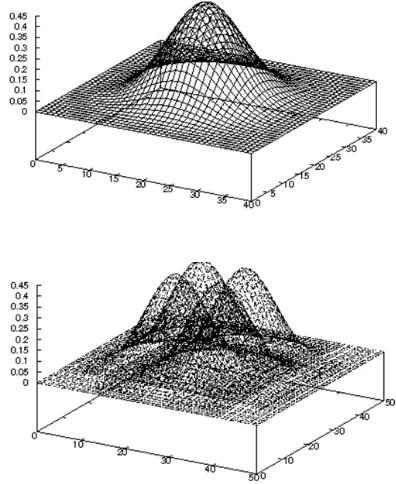
Figure 2.Three dimensional spline functions (order four)
Where {ξw},k=1-r,…,n+r are the knots and n is the total number of intervals for the approximation.The univariate
spline functions are shown in Fig. 1,
where{ξw},k=1-r,…,n+rξ 1,ξ) 2,ξz 3,ξ’ ξ“
ξ” ξ• 4. For the adequate approximation the selection of the knots is quite important.The division by equal intervals cannot always provide the best approximation.
We set the approximation for the three dimensional surface as
. , } &u†…u c† } , —A
† —Q
˜
Where p1, p2 is the total number of basis B-splines {Mi(x)},{Nj(y)} respectively, and these functions have the
support [ ξu!•, ξu ), [ η†!•, η† for the x,y direction respectively.The shape of the three dimensional B-splines are shown in Fig. 2. The upper figure shows a one function
with ‡u š 1 • 10, ›u š 1 • 10, š
1, 2, ^ 5.The lower figure shows four functions with
p1=p2=2, ξu š 1 • 10, ηu š 1 • 10 ,
i=1,2,…,6.The Schoenberg-Whitney condition [12] has to be satisfied, because if there is no sample point in the domain {(x,y)|ξu!• ˆ ‰ ‡u, ›†!•ˆ } ‰ ›†_, then the parameter &u† cannot be determined.
In the equation of integration (4)
4oopA?A8
)
4∑ ∑ &u†t
A•rp
tpA
—A
† —Q
u c† } 8
)
, (7)
4oo|A?A8
)
ž∑ ∑ &u†…u t
AŸ |
t|A
—A
† —Q
u ¡
)
. (8)
We
•¤,w, …u t
AŸ |
t|A •¤),w.Then, the equation (7) (8) can be rewritten as
4oopA?A8
)
6∑xw &¢w•¤,w7),
4oo|A?A8
)
6∑xw &¢w•¤),w7). As a result, the integrations become
{ •¤,—•¤,¥ } tA•r¦p
tpA
tA•r§ p
tpA c†¦ } c†§ } }, (9)
{ •¤),—•¤),¥ }
…u¦ …u§
tAŸ ¦ | t|A
tAŸ §|
t|A }. (10) The sum of equations (9) and (10) will be Kpq which is
the component of m•m nonnegative matrix K that is represented in the equation (5).
3.2Higher Order Empirical Influence Function
We can denote equations (6) as follows
∑ ¨u ; % 0 š 1,2, ^ , , )< 1, (11)
where % &', σ) j. When we denote ¨ 6¨ , ^ , ¨—7', the solution%*of the equation (11) is given by %* Z K* which is the vector of the functional with degree p defined with distribution G as follows:
¨ , Z K K 0.
By replacing the distribution Gwith 1 a K < a©p,we obtain
¨ #, Z 1 a K < a©p \ 1 a K # < a©p # _ 0. (12)
The first order influence function is given in [4].For the higher order influence function, we differentiate the equation (12) with respect to atwice and let a 0, then we obtain
2 ª¨ , Z Kª% ' \©p # K # _ ·ªa \Z Yª ¬ _|¬
< ª%ª%ª)¨ ªZ Yªa |¬ ¬ - K ·ªZ Yªa |¬ ¬
< o®o¯ K ·oA° T±
o¬A |¬ - 0. (13)
Therefore the influence function contains a second order as
oA
o¬A\Z Y¬ _|¬ -² Z) #, #; K .
Recall the equation
o®6=,° ³ 7,
o¯ K # 0,
and the equation (13) can be rewritten as:
2 ´ª¨ #, Z Kª% '|= p< µ ¨, K ¶ Z
< ´ ª%ª% Zª)¨ ; K K¶ Z µ ¨, K Z) 0.
Thus, we obtained
Z)6#, #; K*7
µ ¨, K* ! 42o® =,° ³ , o¯ |= p< oA®
o¯o¯Z ; K* K*8 Z < 2Z .
4. Other Information Criteria
An information criterion for the model56#· ; %*7, obtained by maximizing the penalized log-likelihood function (3)is given by
GIP— 2 log 56# · ; %*7 < 2tr »µ6¨, K*7! ¼ ¨, K* ½ ,
whereµ ¨, K* and ¼ ¨, K* are (m+1)•(m+1) matrices [4]. We adopted the next approximation for the alternative CV [4]
Z6G¾! 7 [ Z G < 1
1 Z #u; G u¿
[ T6G¾7 Z # ; G¾ .
In the equation (1) of ICCV we replaced the %*! with %* Z # ; G¾ and its scheme was called the modified GIC (mGIC) [13],
mGIC 2 log5 ´ ; %* 1Z 6 ; G¾7¶ .
5. Numerical Example
5.1. Surfaces and Samples
We assume two models of the equations of surface I and surface II as follows:
I :# sin 2; < 2cos 2; < }
II :# 1 exp ) < }exp y)
Those topographies are shown in Figure 3.For the estimation, we generated 300 sample coordinates data with the Gaussian noise according to the normal distribution
5.2. Estimation of Parameters
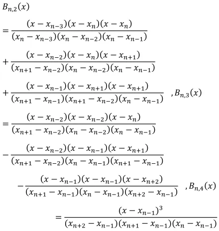
Usually B-splines with order four (degree three) are used in the calculation. Along the x direction, we set the knots x1, x2,^,xpwith four-folded knots at both ends.So the total number of basis B-splines will be p-4.At every interval [xn-1,xn),n=5,6, ^ ,p-3 there exists four basis B-splines which are below.
Figure 3.The topographies of two surfaces
• ,
z
!z !) ! ,
• ,)
!z
!z !) !
< !) y
y !) !) !
< ! y y
y ! y !) ! , • ,z
!) !)
y !) !) !
!) ! y
y !) ! y !
! ! y)
y ! ! y) ! , • ,’
! z
y) ! y ! ! ,
According to the total number of sample data we set 10 - 20 knots along the every axis. We denote the total number of knots (n1,n2) where n1and n2 are the total number of knots along x and ydirections respectively.Also, for every (n1,n2), we tested 100 sets of randomized knots generated uniformly.However, some of them didn't satisfy the Schoenberg-Whitney condition so another set of knots was generated again. Furthermore the equations of matrices made from ill-conditioned sets cannot be solved properly, so we also generated another sets of knots again, testing 100 solvable sets for every (n1,n2).The total number of the basis will be (n1-4)(n2-4) and the total number of the parameters will be (n1-4)(n2-4)+1 which consists of the coefficients of the basis and the variance.For the regularization term, we used (4) and for the numerical calculation, we used (9) and(10). We tested the estimation with various β's which are from10-1 to 10-10 in principle.
5.3. Evaluation of Models
For the evaluation of the obtained parameters we test some criteria such as GICP, mGIC, CV and GCVIF.Those results are shown in Figures and Tables below. Fig. 4 summarize the results of GICP, mGIC, CV and GCVIF over the various values of ƒ for surface I. And Fig. 5 shows the results of four criteria for surface II. The GICP values are monotone decreasing so we cannot determine the optimal parameters in this case.Table 1 and 2 summarize the results of CV in the various values of ƒ.The optimal value, which minimizes the information criterion Cross-Validation (1), determines the number of knots and the value of ƒ. We can determine the optimal parameters which minimize CV,but the repetition is 12100 and it takes about 800 minutes in our simulation for every ƒ and for every surface.
it is 1/23 of the CV.In this approximation of parameters the
Figure 4. Four criteria of Surface I
Figure 5. Four criteria of Surface II
difference between the mGIC and CV is quite small. The correlation coefficient is almost 1.0.For example, when
ƒ=10-5, n1= n2=20, the average of the correlation coefficients over 100 sets of knots is 0.99999611.However, the values of mGIC are monotone decreasing so we cannot determine the optimal parameters in this case.
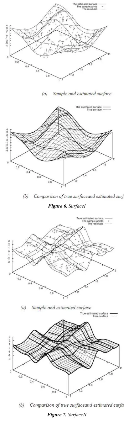
The results of an alternative method GCVIF with influence function (2) for model selection are shown in Table 3 and 4. For the estimation of variance we use the influence function.The selected models with optimal parameters determined by the GCVIF are shown in Fig. 6 and Fig. 7 for surfaces I and II respectively.In Fig. 6 the estimated surface is based on the (13,11) knots. In Fig. 7 the estimated surface is based on the (14,17) knots. In those figures the locations of knots and samples and the residuals are also shown.
5.4. Comparison between the Distributions of Criteria
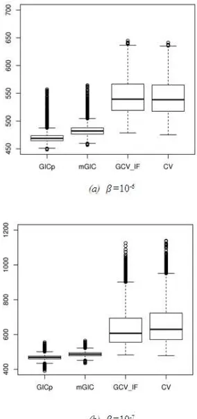
We compare the distributions of four information criteria for the two surfaces I andII.The criteria are improved versions of GICP, CV, mGIC and GCVIF.On the surface I,
we show the Boxplots of four criteria
overƒ=10-4,10-5,10-6,10-7 inFig.8and 9. Similarly on the surface II, we show the Boxplots of four criteria overƒ=10-4,10-5,10-6,10-7 inFig. 10 and 11. We can find from these figures that mGIC is larger than GICP and GCVIF is closer to the CV than others.
Figure 6. SurfaceI
Table1. CV results for Surface I
Total number of knots
x-axis y-axis ββββ σσσσ
2 2 2 2
λ λ λ
λ CV
19 13 1.000E-01 1.85E+00 5.4025E-02 1050.1
19 13 1.000E-02 1.67E+00 5.9798E-03 1021.1
20 17 1.000E-03 9.38E-01 1.0665E-03 859.3
20 17 1.000E-04 3.16E-01 3.1645E-04 560.3
13 11 1.000E-05 3.16E-01 4.4643E-05 468.1
10 11 1.000E-06 2.29E-01 4.3673E-06 475.1
10 11 1.000E-07 2.28E-01 4.3939E-07 478.0
10 11 1.000E-08 2.24E-01 4.4721E-08 478.8
10 11 1.000E-09 2.20E-01 4.5520E-09 479.8
10 10 1.000E-10 2.20E-01 4.5354E-10 486.1
Table2.CV results for Surface II
Total number of knots
x-axis y-axis ββββ σσσσ
2 2 2 2
λ λλ
λ CV
13 13 1.000E-01 3.85E-03 2.60E+01 31.0
18 18 1.000E-02 5.35E-02 1.87E-01 40.2
20 15 1.000E-03 3.22E-01 3.10E-03 537.9
17 20 1.000E-04 1.66E-01 6.03E-04 367.4
20 15 1.000E-05 4.87E-02 2.05E-04 74.3
16 14 1.000E-06 6.37E-03 1.57E-04 -346.1
16 14 1.000E-07 2.30E-03 4.34E-05 -441.1
19 13 1.000E-08 2.77E-03 3.61E-06 -244.2
13 13 1.000E-09 3.85E-03 2.60E-07 25.9
13 13 1.000E-10 3.85E-03 2.60E-08 31.0
Table3.GCVIF results for Surface I
Total number of knots
β β β
β σσσσ
2 2 2 2
λ λ λ
λ GCVIF
x-axis y-axis
19 13 1.000E-01 1.850993 5.40E-02 1050.1
19 13 1.000E-02 1.672307 5.98 E-03 1021.4
20 17 1.000E-03 0.937645 1.07 E-03 857.2
20 17 1.000E-04 0.316010 3.16 E-04 556.9
13 11 1.000E-05 0.224000 4.46 E-05 470.0
12 10 1.000E-06 0.214460 4.66 E-06 478.4
10 11 1.000E-07 0.227586 4.39 E-07 481.9
10 11 1.000E-08 0.223611 4.47 E-08 484.3
10 10 1.000E-09 0.220486 4.54 E-09 487.3
10 10 1.000E-10 0.220486 4.54 E-10 487.3
Table4.GCVIF results for Surface II
Total number of knots
β β β
β σσσσ
2 22 2
λ λλ
λ GCVIF
x-axis y-axis
18 11 1.000E-01 0.407434 2.45 E-01 596.9
20 19 1.000E-02 0.397532 2.52 E-02 591.1
20 15 1.000E-03 0.355688 2.81 E-03 536.8
17 20 1.000E-04 0.165862 6.03 E-04 363.9
10 10 1.000E-05 0.227627 4.39 E-05 60.3
14 17 1.000E-06 0.005844 1.71 E-04 -463.0
14 17 1.000E-07 0.001890 5.29 E-05 -659.3
14 17 1.000E-08 0.001712 5.84 E-06 -582.7
13 13 1.000E-09 0.003851 2.60 E-07 -549.8
Figure 8.Boxplotsfor four criteria of surface I
Figure 9. Boxplotsfor four criteria of surface I
Figure 10. Boxplotsfor four criteria of surface II
7. Conclusion
As the value of ƒ decreases, the residual variance reduces and the information criterion GICp also reduces
monotonously. As a result, the GICp cannot determine the
optimum model in both surfaces.The method for minimizing the cross-validation (CV) can determine the optimal values for two surfaces.The result of computation shows the excellence of the criterion CV, but it requires a large amount of computational costs.
For the parameter estimation the alternative method mGIC by the information function works well.However, the total number of parameters is so many (more than 36 and less than or equal to 257) that occasionally the estimated values are quite different from the sample value.Those samples make the value of mGIC worse and consequently we cannot determine the optimum model by this criterion in both surfaces.To overcome this difficulty the GCV is quite useful.To improve the property of GCV we use the influence function to estimate the variance of
n-1 samples.We can recognize the superiority of GCVIF
which can determine the optimum model and can approximate the distribution of the CV very well and it requires small computation.
We propose GCVIFas an improved GCV criterion. This conclusion is a theory obtained through a large number of simulation tests.From the results of these tests of GCVIF
criterion on surface I and surface II, we can see that the GCVIF criterion is more stable than the CV, GIC and
mGIC, and we can also see that the GCVIF criterion
includes their informations.
References
[1] Konishi, S., Kitagawa, G. (1996). "Generalised information criteria in model selection.",Biometrika, 83, 875–890.
[2] Stone,M., "Cross-validatory choice and assessment of statistical predictions (with discussion)", Journal of the Royal Statistical Society, Series B, 36 (1974), 111–147.
[3] Ueki, M. and Fueda, K. (2010)."Optimal Tuning Parameter Estimaiton In Maximum Penalized Likelihood Method",
Annals of the Institute of Statistical Mathematics, 62, 413-438.
[4] Konishi, S., Kitagawa, G. (2008). "Information Criteria and Statistical Modeling", Springer Science+Business Media, LLC.
[5] Good, I. J. and Gaskins, R.A.(1971). "Non parametric roughness penalties for probability densities", Biometrika, Vol. 58. pp. 255-277.
[6] Good, I. J. and Gaskins, R.A.(1980). "Density estimation and bump hunting by the penalized likelihood method exemplified by scattering and meteorite data", Journal of American Standard Association, Vol. 75. pp. 42-56.
[7] Green, P. J., Silverman, B. W.(1994). "Nonparametric Regression and Generalized Linear Models", Chapman and Hall, London.
[8] Umeyama, S. (1996). "Discontinuity extraction in regularization using robust statistics", Technical report of IEICE.,PRU95-217 (1996). pp. 9-16.
[9] Cox, M.G.(1972). "The numerical evaluation of B-splines",
J. Inst. Math. Appl., 10, pp.134-149.
[10] Cox, M.G.(1975). "An algorithm for spline interpolation", J. Inst. Math. Appl.,15, pp.95-108.
[11] de Boor, C.(1972). "On calculation with B-splines", J. Approx. Theory, 6, pp.50-62.
[12] Schoenberg, I. J., Whitney, A.(1953). "On Pólya frequency functions III", Trans. Amer. Math. Soc, Vol. 74. pp. 246-259, pp. 246-259.