A Packet Buffer Evaluation Method Exploiting
Queueing Theory for Wireless Sensor Networks
Tie Qiu1,2, Lin Feng2, Feng Xia1*, Guowei Wu1, and Yu Zhou1
1 School of Software, Dalian University of Technology, 116620 Dalian, China
[email protected]; [email protected]
2 School of Innovation Experiment, Dalian University of Technology, 116024 Dalian, China
Abstract. In large-scale wireless sensor networks (WSNs), when the consumption of hardware is limited, how to maximize the performance has become the research focus for improving transmission quality of service (QoS) of WSNs in recent years. This paper presents a new evaluation method for packet buffer capacity of nodes using queueing network model, whose packet buffer capacity is analyzed for each type node, when it is in the best working condition. In order to evaluate congestion situation in the queueing network, and to get real effective arrival rates and transmission rates in the model, holding nodes were added in the queueing network model, and equivalent queueing network model is expanded. We establish an M/M/1/N type queueing network model with holding nodes for WSNs and design approximate iterative algorithms. Experimental results show that the model is consistent with the real data.
Keywords: wireless sensor networks, queueing network model, blocking, packet buffer capacity, node utilization.
1.
Introduction
Wireless sensor networks (WSNs) are successfully applied in intelligent transportation, monitoring environment, location and other fields. They consist of tiny sensing devices that have limited possessing and computation capabilities, and can collaborate real-time monitoring, sensing, collecting network distribution of the various environments within the region or monitoring object information [1,2,3]. WSNs of distribution regions are composed of sink nodes [4,5,6], transmission nodes and boundary nodes [7]. The performance of each type node will affect the overall network performance in WSNs. Throughput and utilization [8,9,10] of the nodes in the lifetime [11,12] are the main evaluation performance indicators of WSNs. The
packet buffer capacity of nodes is an important factor in utilization of network nodes [13]. If a node of WSNs is blocked, and packet buffer set too small, the entire network data transmission and processing efficiency is not high. Therefore, when the consumption of hardware is limited, how to optimize the node packet buffer size and maximize the performance for WSNs has become a research focus for improving the Quality of Service (QoS) of WSNs transmission in recent years.
In this paper, we consider that packet buffer capacity corresponds to the length of the waiting queue in the established limited capacity of the queueing network model. When the length of the waiting queue reaches the maximum, the node is blocked in the queueing network model. Therefore, a typical WSN is modeled by M/M/1/N type queueing network model. The method of modeling based on topology of nodes in WSNs and performance analysis of the packets buffer capacity have been proposed. According to the topology of WSNs and operational characteristics, arrival, transferring and leaving relationships of transmission nodes, boundary nodes and sink node are analyzed, and data flow balance equations are obtained. In order to evaluate the congestion situation in the queueing network, and get real effective arrival rates and transmission rates in the model, holding nodes were added in the queueing network model and equivalent queueing network model is expanded. By analyzing the queueing model with blocking probability, to obtain the performance index of system when it is in steady state, approximate iterative algorithms are designed. The performance parameters of nodes model in the WSNs are calculated using limited iteration times. The optimal values for packets buffer sizes settings are obtained for transmission nodes, boundary nodes and sink nodes.
Networks
2.
Related Work
When the hardware has been implemented, it is difficult to adjust the node's hardware resources in accordance with specific needs. Therefore, researchers have proposed the need for large-scale WSN nodes modeling method [14]. Through performance evaluation of pre-setting nodes, optimal parameters of allocation for the hardware nodes are obtained. The current modeling method based on Petri nets [15,16,17] is suitable for macro-modeling, but it is not a specific modeling technique for large-scale WSNs. Queueing network is an effective system-level modeling method, which is widely used in the modeling and performance analysis of computing and communication systems [18,19]. It has many advantages that include a highly abstract and rich theory for modeling.
In recent years, researches have made some progress on analyzing and improving network performance in the application of finite capacity queueing networks. Bisnik et al. [20] modeled random access multi-hops wireless networks as open G/G/1 queueing networks and used diffusion approximation in order to evaluate closed form expressions for the average end-to-end delay. In [21,22], Kouvatsos and Awan described the priorities and blocking mechanisms with open-loop queueing network performance analysis, and queueing network parameters on the approximation and error estimates. Özdemira et al. [23] presented two Markov chain queueing models with M/G/1/K queues, which have been developed to obtain closed-form solutions for packets delay and packets throughput distributions in a real-time wireless communication environment using IEEE 802.11 DCF. Mann et al. [24] developed a queueing model for analyzing resource replication strategies in WSNs, which can be used to minimize either the total transmission rate of the network or to ensure that the proportion of query failures does not exceed a predetermined threshold. In [20], Liehr et al. introduced enhancements to the standard of extended queuing network models, which allow the modeling and the simulation of inter-process communication and highlight the benefits granted by their enhanced EQN approach. However, these researches don’t address the packet buffer capacity of nodes and how to set the buffer size to derive the optimal performance of the nodes in WSNs.
3.
Problem Statement
Data packets are transmitted and processed in collaboration by the sink nodes, transmission nodes and boundary nodes. For a large scale WSN, a queueing network model can be used to analyze its performance [25, 26]. But how to configure resources to find the best value hardware using trends of changing the parameters of performance is an important reference for node design. The definition of the threshold of node buffer capacity is given below:
Definition 1. When the queueing network system is stable, node’s
to be processed. Buffer size value at the moment is called the node threshold, denoted by NT.
4
1 2
3
Boundary Node
Transmission Node Sink Node
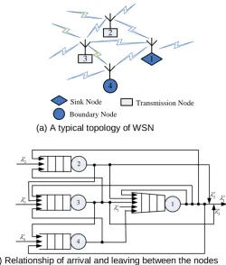
(a) A typical topology of WSN
4 2
1 3
e
2
e
3
e
4
e
1
o
2
o
3
o
1
(b) Relationship of arrival and leaving between the nodes
Fig. 1. Topology and node transfer of the WSN.
In WSNs, for any node buffer size, we make the following discussion: (i) If Ni NT, node queue length will never be processed over the buffer
capacity when a system is in a steady state. Therefore, the packets that have not been timely processing data will be placed in the packet buffer. Newly arrived packets will not cause the blocking node server.
(ii) If Ni NT, when the packet buffer of node is full, the link paths that
include the nodes are blocked, and lead to the processing efficiency of the whole WSN down. On the other hand, when the link path is blocked, all the nodes are in an active state in the link path. Therefore, energy consumption of the node is larger, and individual nodes are invalidated due to energy exhaustion.
Networks relationship between the node queues as shown in Figure 1(b), where e
i
is the independent external Poisson arrival rate of node i and o i
is the leaving rate after the completed service of node i. (Note: Boundary node does not include o
i
).
In practice, the task content of sink nodes, transmission nodes and boundary nodes is different. Therefore, its consumption of hardware resources will be different. For example, in Figure 1(b), the arrival rate of sink node 1 packets is the maximum. Therefore, finding a way to properly evaluate its performance becomes very important. That is, how to set the packet buffer capacity of wireless sensor nodes, in order that each node has the highest speed of data processing and throughput. Thus, the best parameters between the utilization of node and consumption of hardware buffer capacity will be found. In order to facilitate the analysis of queueing network model for WSNs, some symbols are defined in Table 1.
Table 1. Definition of symbols
Symbol Description
i, j, k, d Node No. in the queueing network.
M Total number of paths in the queueing network. N Size of packet buffer capacity
i
Arrival rate of node i.
i
Service rate of node i.
i
Utilization of node i.
pi Steady-state probability of arrival node i.
o i
p Leaving probability from node i.
pij Probability of from node i to node j.
S State of node.
Ti Monitoring cycle of i-th times in WSN. A Aggregate of all the holding nodes.
ij
pb Blocking probability from node i to node j.
e i
pb Independent external Poisson arrival blocking probability of node i.
a i
pb Total arrival blocking probability of node i.
4.
Open Queueing Network Analysis for WSN Model
queueing network model is obtained. Therefore, analysis of the blocking queueing network is possible.
4.1. Open Queueing Network
A typical open queueing network composed of WSN is consistent with a flow balance equation. According to the theorem for flow balance equation [25,27], we can give Corollary 1 and Corollary 2 for any WSN.
Corollary 1. For the transmission node, arrival node and leaving node in the queueing network of WSN, the number of all possible packets leaving the node i equals that of the arrival number in the state.
1
1
m d
e o
i k ki i if i i
i f j
p
p
p
(1)
Proof: Using reductio ad absurdum, suppose the number of packets
entering the node i is not equal to the number of packets leaving the node i, then according to the flow balance equation, there must be packets with probabilitypii 0 in the self-loop. This is in contradiction with the fact that transfer node, arrival node and leaving node service is the order of one-way services in WSNs. Therefore, the Corollary 1 is established. □
Corollary 2. For the sink node in the queueing network of a WSN, the sum
of the arrival packet and self-loop packet equals that of the sum of the leaving packet for node i in the state.
1
1
m d
e o
i k ki i ii i if i i
i f j
p
p
p
p
(2)Proof: For the sink node in the queueing network of a WSN, data transmission between nodes requires a very high accuracy. When the data packets validation is not correct, we should have re-transmission processed until the correct calibration data is received. Therefore, the phenomenon of self-loop appears in the node i. Increased the number of arriving packet is equivalent to ipii. Therefore, we can get the sum of arrival packet as equation (3).
1
1
m e
i i k ki i ii
i
p
p
(3)According to flow balance equation [25,27], we can deduce that the flow balance equation (2) is established. □
Networks monitoring and sleeping, as a premise in meeting the required monitoring conditions. Switching between states of nodes is shown in Figure 2.
Sleeping Monitoring Sleeping … …
Ti+1
Sleeping Monitoring
Ti
…
Fig. 2. Switching between states of nodes.
Next, we give the definition of the longest monitoring cycle of node i.
Definition 2. For all nodes in WSNs, the wake-up from a sleeping state into the monitoring state, and then entry into another sleep experienced by far the longest time is known as the longest monitoring cycle of WSN nodes.
} ..., , ..., , ,
max{ 1 2 i N
m
i T T T T
T (4)
In WSNs, each node has a packet capacity. If the packet buffer size is set too large, would be a waste of resources. Conversely, if the data packet buffer size is set too little, block of system will be increased. We give the theorems for packet queue length of sink nodes and transmission nodes.
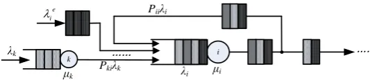
i
μi
λi
Piiλi
Pkiλk
……
k
μk
λk
e i
……
Fig. 3. Transmission relation of packet queue for sink node i.
Theorem 1.For any sink node i in WSNs, packet queue length of sink node is
m i
L , then the following relationship is obtained.
1
1
(1
)
m m
e i
i k ki m ii i
i i
L
p
p
T
(5)Transmission relation of packet queue for sink node i in WSNs is shown in Figure 3. We give the proof of Theorem 1 below.
Proof: For sink node i in WSNs, according to Corollary 2, the data packets arrival rate is obtained by equation (6).
1
1
m e
i i k ki i ii i
p
p
(6)In the time period, the arrival number is Xi given by equation (7).
i m i i T
At this time, the service rate is i. The number of the data packets is Yi given by Equation (8) after completion of the service.
i m i i T
Y (8)
Therefore, packets queue length of node i is m i
L , which is the difference between the number of effective arrival and leaving, and minus the number of packets being processed.
1
i i
m i X Y
L (9)
Putting Equations (6), (7), and (8) into Equation (9) will result in Equation (5). Therefore, Theorem 1 is proved. □
Theorem 2. For any transmission node i in WSNs, if packets queue length of
transmission node is m i
L , then the following relation is obtained.
1
1
m m
e i
i k ki m i
i i
L
p
T
(10)Proof of Theorem 2 is relatively simple, using Corollary 1, and with reference to the proof of Theorem 1.
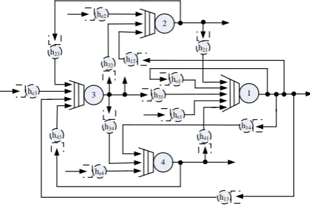
4.2. Equivalent Queueing Network Model
The packet buffer size should be consistent with the length of the queue in the queueing model of WSNs. When the queue length reaches the maximum, the packet streams are stopped, resulting in queueing network being blocked [31,32]. When a data packet transfers from one queue to another queue and if the path is full, the packet will be blocked in by the just completed service in the queue. Then the blocked node cannot handle any other data packets until the destination node services, where there is a free packet buffer before they can lift the blocking. This situation is called Transfer Blocking.
Networks Intervals between the arrival time accord with the exponential distribution. Thus, we calculate the real effective arrival rate nodes, and its performance evaluation is possible.
1 2
4 3
he3 h
31 h32
h34
h23 h21
h41 h14 h12 h43 h13 he2 he4 ho1 he1
Fig. 4. Queueing network model with holding nodes.
4.3. Queueing Model Analysis with Blocking Probability
When the holding nodes are added in queueing network, the packets that did not receive timely services are stored in the queue of holding nodes, as waiting for an empty target node. Total effective arrival rate is equal to the external arrival rate e
j
and the internal arrival rate of nodes 1 2
, ,..., A
i i i after considering blocking nodes. Then, the queueing network model with blocking probability is shown in Figure 5. Below we discuss flow balance of arrival and leaving data packets in the queueing network model.
hej i1 e j pb e j ) 1 ( e j pb e j e j 1 i j pb 1 i j ) 1 ( i1
j
pb
h i1j
1 i j iA A i j pb A i j ) 1 ( A i j pb Q i j h iAj
… j haj a j pb j j e j pb e j 1 i j pb 1 i j
… (1 )
a j pb j ) 1 ( e j pb e j A i j pb A i j ) 1 ( 1 i j pb 1 i j … ) 1 ( A i j pb A i j
(a) Queueing network model with multiple arrival nodes
(b) Equivalent queueing network model
Fig. 5. Queueing network model with blocking probability.
Therefore, the external effective arrival rate ej of node j is obtained as in
Equation (11).
(1 )
e e e
j j pbj (11)
The effective data packets stream from node i to node j as shown in Equation (12). ) 1 ( ij ij i
ij
p pb
(12)Let j be the effective internal arrival rate of node j, which is equal to the
sum of effective internal arrival rate from independent internal nodes
1 2
, ,..., A
i i i .
A i ij j (13)
Total effective arrival rate with probability pbaj of node is obtained by
Equation (14).
) 1 ( aj j j pb
(14)
According to Corollary 1 and Corollary 2, we can obtain a flow balance equation of queueing network with blocking.
j e
j
j
(15)
Equation (16) is derived from applying equations (11) (12) (13) (14) into Equation (15). ) 1 ( ) 1 ( ) 1
( ij
A i ij i e j e j a j
j pb pb
p pb
(16)
In order to obtain the effective arrival rate of node j, the calculations of blocking probability pbij ,
a j
pb and e j
pb are needed. The three blocking probabilities are calculated, the specific derivation is shown as in [37].
Networks
5.
Total Arrival Rate of Nodes and Approximate Algorithm
Blocked nodes are released by adding holding nodes of infinite capacity in the queueing network model. Processing time of blocked node is the blocked time, and thus we can describe arrival and service process of nodes in the equivalent queueing network model. In a lot of practical application and engineering experiments, we found that when WSN node communication enters into a stable state, the average arrival rate of node tends to be a constant value. We designed an iterative method, such as shown in Algorithm 1. We set initial values to the network status, and then gradually revised the last time arrival rate by our iterative method. In the end, a system was approaching to reach equilibrium. The reduction algorithm is as follows.
Algorithm 1
Begin
Step 1. According to transition probability, each node connection in the queueing network model is obtained. External arrival rate e
j
(j is the number of nodes) is determined.
Step 2. Initialize n nodes with the total arrival rate 0
j (1 j m).
Step 3. For queue j in queueing network, calculate the arrival ratej of node j:
Step 3.1. If node j is a transmission node or boundary node,
1
1
m e
j j i ij
i
p
(17)go to Step 3.3. Otherwise, it is executed orderly.
Step 3.2. node j is sink node,
1 1
1
j
m e
j k ki i ii i
p
p
(18)Step 3.3. The outputting rate of node j is calculated by Corollary 1 and Corollary 2.
Go to Step 3.1, until the difference of the internal arrival rate for two computing (before and after) is less than a certain value (error limit of our calculations is 10-4).
Step 4. After calculating the arrival rate of all nodes, if the difference of the internal arrival rate for two computing values is less than a value (10-4), go to Step 5. Otherwise, use 1
j
instead 0
j
iterative calculation.
Step 5. Return the total arrival rate n j
of each node.
End
The time complexity of Algorithm 1 is O(n*m), where m is the number of queueing network nodes and n is the number of iterative algorithms.
The total arrival rate of each node was obtained by Algorithm 1, but it is not the effective arrival rate, because the blocking probability of the nodes is not considered. Next we will have the numerical results of Algorithm 1 as the initial value of Algorithm 2, and then solve the blocking probability and system performance indicators. The reduction Algorithm 2 is as follows.
The calculation of Algorithm 2 mainly focused on the loop in Steps 3 to 6 of the cycle. The time complexity of Algorithm 2 is O(n*m*N), where N is the packet buffer size of node. When the iterative algorithm converges, the WSN performance parameters are outputted. According to that we can predict the actual operation of WSNs. Thus, the hardware design for the WSN node is guided by the performance parameters.
Algorithm 2
Begin
Step 1. The equivalent queueing network model is expanded by adding holding nodes in wireless sensor queueing networks. The total arrival rate of Algorithm 1 is the initial input value of Algorithm 2 for each node.
Step 2. Blocking probabilities of each node are initialized, and means and variances of internal arrival time are calculated.
Step 3. Calculate the utilization and steady-state probability of the nodes, where ni {1,2,..., }N , that means the number of data packet buffer of each node. When the system reaches a steady state, we assume that the probability of queue i in state ni is p ni( )i , which is obtained by:
1
(1 )
( ) 1
i
n
i i N
p n (19)
where i
i i
. Specific derivations of Equation (19) can be found in
[38,39]. According to Jackson’ theorem [30], the status of node i and the status of all other nodes are independent. Thus, we can get the steady-state probabilities of any node in the link path.
Step 4. Calculate the blocking probabilities.
Networks using blocking probabilities.
Step 6. If the difference of the internal arrival rate for two computing (before and after) is less than a certain value (error limit of our calculations is 10-4), then go to Step 7. Otherwise go to Step 3 followed by iterative calculation.
Step 7. Return to the node utilizations with a blocking when system is stable.
End
6.
Numerical Calculation and Experimental Results
According to the preceding analysis, we studied a WSN topology for temperature monitoring. The performance parameters of WSN nodes are calculated using the iterative algorithm proposed in Section 5. By setting different packet buffer capacity sizes of nodes, the relationship curves between utilization (i) and data packet buffer size (Ni) for transmission nodes, boundary nodes and sink node are obtained. In order to rationally allocate resources, the maximum utilizations of nodes are ensured within limited resources. According to the relationship curves between utilization (i) and data packet buffer size (Ni), the values of packet buffer capacity size for transmission nodes, boundary nodes and sink nodes are set.
6.1. A WSN Topology
We have designed the WSNs for temperature monitoring. Its typical topology is shown in Figure 6. It consists of many clusters, each of which comprises a mixed structure from the ring and star network topologies. Information between clusters is communicated by sink nodes.
size to obtain the optimal performance of the nodes for hardware design of WSNs is a practical application problem that needs to be solved.
2
6
3
7
5
1 4
Boundary
Cluster1 Cluster2
Fig. 6. A WSN topology for temperature monitoring.
6.2. Node Transition Probabilities and Total Arrival Rate
The node transition probabilities for the topology of Figure 6 are obtained from packet statistics in the engineering practice of WSNs for temperature monitoring. Thus the transition probability matrix is as follows.
0 0.2 0 0 0 0.2 0.5
0.2 0 0.2 0 0 0 0.5
0 0.2 0 0.2 0 0 0.5
0 0 0.2 0 0.2 0 0.5
0 0 0 0.2 0 0.2 0.6
0.2 0 0 0 0.2 0 0.6
0.1 0.1 0.1 0.1 0.1 0.1 0
P (20)
Networks
Table 2. Arrival rate for each node in the time Tim Node
number
External arrival rates e
i (p/s)
Total arrival Rates i (p/s)
1 10 29.6577
2 10 31.1161
3 10 31.1161
4 10 29.6577
5 3 22.3661
6 3 22.3661
7 2 89.6131
According to the input of the external arrival rates, the total arrival rate of node i can be calculated using Algorithm 1, as shown in Table 2.
6.3. Evaluation for Packet Buffer Capacity of Nodes
In WSNs, packet buffer capacity of nodes settings that affects the efficiency of the whole network system is an important factor. If packet buffer capacity is too small it will cause serious blocking to some link paths of the system, and lead to a low efficiency of data processing and transmission. If packet buffer capacity is too large, it will take up too much of the hardware resources, resulting in an increased cost of the hardware node. And the energy consumption will increase, causing a link failure to individual nodes due to energy depletion. Therefore, we design hardware nodes that make the data packet buffer capacity to reach the optimal settings.
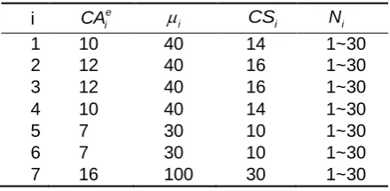
Other input parameters of queueing network model for wireless sensor are shown in Table 3, where e
i
CA is the independent external Poisson arrival Variance of node i, i is the service rate of node i, CSi is the service variance of node i and Ni is the size of packet buffer capacity which ranges from 1 to 30.
Table 3. Input parameters for model
i CAie i CSi Ni
1 10 40 14 1~30
2 12 40 16 1~30
3 12 40 16 1~30
4 10 40 14 1~30
5 7 30 10 1~30
6 7 30 10 1~30
According to of the approximate iterative Algorithm 2 in Section 5, packet buffer size (Ni) and node utilization (i) are calculated.
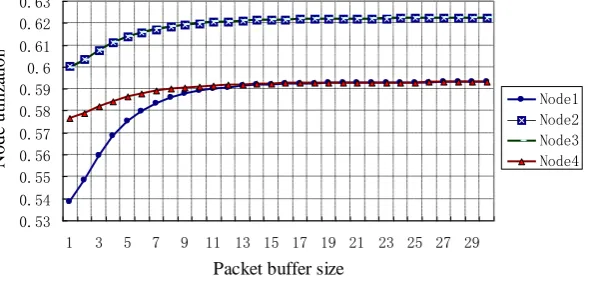
0.53 0.54 0.55 0.56 0.57 0.58 0.59 0.6 0.61 0.62 0.63
1 3 5 7 9 11 13 15 17 19 21 23 25 27 29
Packet buffer size
N
o
d
e
u
ti
li
za
ti
o
n
Node1 Node2 Node3 Node4
Fig. 7. Relationship curves between utilization and buffer size for transmission nodes. The relationship curves between utilization and packet buffer size for transmission nodes are shown in Figure 7. In WSNs for temperature monitoring, node 1, node 2, node 3 and node 4 are the transmission nodes, in which the main function of the network is to collect data and transfer it to other nodes. With the increase of packet buffer size, increased speed of node 1 is the fastest, increased speed of node 4 has slowed down compares to other three nodes. When the packet buffer sizes are increased toN1N4 14, curves for nodes 1 and 4 coincide. Next, with the increase of packet buffer size, the curves in almost horizontal axis tend to become parallel. At this time, if we increase the packet buffer sizes, utilization for nodes will not have any impact. This point can be set as the value of packet buffer size then the node utilization is optimal. From point of view for the layout of the WSNs, nodes 1 and 4 are adjacent to the boundary nodes, transmission rates of data packets are almost the same. Therefore, when the system reaches equilibrium, packet buffer sizes in use become the same.
Networks
0.38 0.39 0.4 0.41 0.42 0.43 0.44 0.45 0.46
1 3 5 7 9 11 13 15 17 19 21 23 25 27 29
Packet buffer size
N
o
d
e
u
ti
li
za
ti
o
n
Node5 Node6
Fig. 8. Relationship curves between utilization and buffer size for boundary nodes. The relationship curves between utilization and packet buffer size for boundary nodes are shown in Figure 8. With the increase of packet buffer size, beginning curves are relatively steep. The increased speed of curve for node 5 is the fastest; the increased speed of curve for node 6 has slowed down compared to curve for node 5. According to this situation, we can speculate that, when node 5 is set to a smaller packet buffer size, a more serious blocking occurred in the link paths for the node, resulting in relatively low node utilization. When the packet buffer sizes increased to N5N613, curves for nodes 5 and 6 are coincidence. And following the increase of packet buffer size, the curves in almost horizontal axis tend to become parallel. At this time, if we increase the packet buffer sizes, utilization for nodes will not have any impact. If this point can be set as the value of packet buffer size, then the node utilization is optimal. From the point of view of the layout of the WSNs, nodes 5 and 6 are located on the outside of the WSN, and they are boundary nodes. The transmission rates of data packets are almost the same. Therefore, when the system reaches equilibrium, the packet buffer sizes in use are the same.
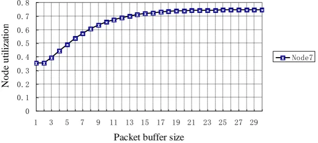
0 0.1 0.2 0.3 0.4 0.5 0.6 0.7 0.8
1 3 5 7 9 11 13 15 17 19 21 23 25 27 29
Packet buffer size
N
o
d
e
u
ti
li
za
ti
o
n
Node7
For sink node 7, on the one hand, it is responsible for collecting the date packets of adjacent transmission nodes and boundary nodes. On the other hand, information between clusters is communicated, and a partial data processing is completed by sink node. The relationship curves between utilization and packet buffer size for sink node are shown in Figure 9.
With the increase of packet buffer size, beginning curves are relatively steep. As per this situation, we can speculate that, when sink node 7 is set to a smaller packet buffer size, its utilization is relatively low. After the packet buffer sizes are increased to N719, and following this, the curves in almost horizontal axis tend towards parallel. At this time, if we increase the packet buffer sizes, utilization for nodes will not have any impact. If this point can be set as the value of packet buffer size, then the node utilization is optimal.
6.4. Comparison of Experimental Data and Model Calculation Data
According to the size of the nodes through the analysis of packet buffer size in Section 6.3, the experimental environment was designed. The packet buffer sizes for transmission nodes are set as N1N4 14 , N2 N3 11 , respectively. The packet buffer sizes for boundary nodes are set as
5 6 13
N N , respectively. The packet buffer size for sink node is set as
7 19
N . The simulation environment using NS2 software combined with random arrival derived the algorithm [39]. The experimental simulation for arrival rate of node with holding nodes was carried out. Figure 10 shows the comparison of nodes between the effective arrival rates.
0 10 20 30 40 50 60 70 80 90 100
A
rri
va
l ra
te
1 2 3 4 5 6 7
Node number
ideal calculated value of the infinite capacity
calculated values with "holding nodes" of limited capacity
measurement values of the experimental data
Networks In Figure 10, the arrival rates of the three situations are described: (i) Assuming queueing network model for wireless sensor works in an ideal state, the blocking probabilities {pbij,pbaj ,pbej} always equal 0, which is called the ideal calculated value of the infinite capacity nodes. (ii) Queueing network model for wireless sensor maintained by adding a finite number of nodes (based on the values obtained in Section 6.3), considering the given blocking probabilities {pbij,pbaj ,pbej}, the values of the effective arrival rate are calculated, these are called the calculated values with holding nodes of limited capacity. (iii) Experimental environment is created and random function for arrival rate is designed. Therefore, the actual arrival rates are obtained by statistical calculation, these are called the measurement values of the experimental data. Figure 10 clearly describes the comparison of data among the three situations. We can see that errors between the ideal calculated value of the infinite capacity nodes and the calculated values with holding nodes of limited capacity are very small, the maximum error being 6.12%. This proves that by adding finite holding nodes to a queueing network model, and obtained equivalent queueing network model can replace the infinite capacity model for performance analysis. The maximum error between the measurement values of the experimental data and the calculated values with holding nodes of limited capacity is 9.56%. As in the model calculation error is less than 10%, almost consistent indicators for equivalent queueing network model can be obtained with the actual operation of the WSN.
7.
Conclusions
model, provides a theoretical basis for design of high cost-effective hardware nodes for modeling large-scale WSNs. This work has important guiding significance for hardware design and performance evaluation of WSNs system.
This paper presents a modeling for only a single-server model in WSN and a method for calculating the packet buffer capacity size of nodes. However, the sink node requires a higher performance. Recently, there has been convergence of multiple processor nodes that can be used for M/M/m/N queues, which are also multi-server queues. In addition, for large-scale WSNs, if the clusters are set to be the priority, it will effectively improve the performance of WSNs. This will be our follow-up research.
Acknowledgment. This work was supported in part by Natural Science Foundation of China under Grant No. 61173163, 60903153 and 61173179, Program for New Century Excellent Talents in University (NCET-09-0251), the Fundamental Research Funds for the Central Universities, and the SRF for ROCS, SEM.
8.
References
1. Onur, E., Ersoy, C., Deliç, H., Akarun, L.: Surveillance with wireless sensor networks in obstruction: Breach paths as watershed contours. Computer Networks, Vol. 54, No. 3, 428-441. (2010)
2. Lasassmeh, S., M., Conrad, J., M.: Time synchronization in wireless sensor networks: A survey. Conference Proceedings-IEEE SoutheastCon 2010: Energizing Our Future, 242-245, Concord. (2010)
3. Son, J., H., Lee, J., S., Seo, S., W.: Topological key hierarchy for energy-efficient group key management in wireless sensor networks. Wireless Personal Communications, Vol. 52, No. 2, 359-382. (2010)
4. Yick, J., Mukherjee, B., Ghosal, D.: Wireless sensor network survey. Computer Networks, Vol. 52, No. 12, 2292-2330. (2008)
5. Akyildiz, I., F., Su, W., Sankarasubramaniam, Y., Cayirci, E.: A survey on sensor networks”, IEEE Communications Magazine, Vol. 40, No. 8, 102-114. (2002) 6. Alnabelsi, S., H., Almasaeid, H., M., Kamal, A., E.: Optimized sink mobility for
energy and delay efficient data collection in FWSNs. 15th IEEE Symposium on Computers and Communications, 550-555, Riccione. (2010)
7. Sheu, J., P., Sahoo, P., K., Su, C., H., Hu, W., K.: Efficient path planning and data gathering protocols for the wireless sensor network. Computer Communications, Vol. 33, No. 3, 398-408. (2010)
8. Gao, S., Zhang, H., Song, T., Wang, Y.: Network lifetime and throughput maximization in wireless sensor networks with a path-constrained mobile sink. 2010 International Conference on Communications and Mobile Computing, 298-302, Shenzhen. (2010)
9. Eun, D., Y., Wang, X.: Achieving 100% throughput in TCP/AQM under aggressive packets marking with small buffer. IEEE/ACM Transactions on Networking, Vol. 16, No. 4, 945-956. (2008)
Networks 11. Vupputuri, S, Rahuri, K., K., Murthy, C., S., R.: Using mobile data collectors to improve network lifetime of wireless sensor networks with reliability constraints. Journal of Parallel and Distributed Computing, Vol. 70, No. 7, 767-778. (2010) 12. Han, J., Choi, S., Park, T.: Maximizing lifetime of cluster-tree ZigBee networks
under end-to-end deadline constraints. IEEE Communications Letters, Vol. 14, No. 3, 214-216, (2010)
13. Subramanian, R. Fekri, F.: Unicast throughput analysis of finite-buffer sparse mobile networks using Markov chains. 46th Annual Allerton Conference on Communication, Control, and Computing, 1161-1168, Monticello. (2008)
14. Li, G., H., Zhu, C., M., Li, X.: Application of Chaos theory and Wavelet to Modeling the Traffic of Wireless Sensor Networks. 2010 International Conference on Biomedical Engineering and Computer Science, 1-4, Wuhan, (2010)
15. Escheikh, M., Barkaoui, K.: Opportunistic MAC layer design with Stochastic Petri Nets for multimedia ad hoc networks. Concurrency Computation Practice and Experience, Vol. 22, No. 10, 1308-1324. (2010)
16. Moon, C. Chung, W.: Design of navigation behaviors and the selection framework with generalized stochastic petri nets toward dependable navigation of a mobile robot. 2010 IEEE International Conference on Robotics and Automation, 2989-2994. Anchorage. (2010)
17. Shareef, A., Zhu, Y.: Energy modeling of processors in wireless sensor networks based on petri nets. 37th International Conference on Parallel Processing Workshops, 129-134, Portland. (2008)
18. Strelen, J., C., Bark, B., Becker, J., Jonas, V.: Analysis of queueing networks with blocking using a new aggregation technique. Annals of Operations Research, No. 79, 121-142. (1998)
19. Liehr, A., W., Buchenrieder, K., J.: Simulating inter-process communication with Extended Queueing Networks. Simulation Modelling Practice and Theory, Vol. 18, No. 8, 1162-1171. (2010)
20. Bisnik, N., Abouzeid, A., A.: Queuing Network Models for Delay Analysis of Multihop Wireless Ad Hoc Networks. Ad Hoc Networks, Vol. 7, No. 1, 79-97. (2009)
21. Kouvatsos, D., Awan, I.: Entropy maximisation and open queueing networks with priorities and blocking. Performance Evaluation, Vol. 51, No. 2-4, 191-227. (2003)
22. Awan, I.: Analysis of multiple-threshold queues for congestion control of heterogeneous traffic streams. Simulation Modelling Practice and Theory, Vol. 14, No. 6, 712-724. (2006)
23. Özdemira, M., McDonald, A., B.: On the performance of ad hoc wireless LANs: A practical queueing theoretic model. Performance Evaluation, Vol. 63, No. 11, 1127-1156. (2006)
24. Mann, C., R., Baldwin, R., O., Kharoufeh, J., P., Mullins, B., E.: A queueing approach to optimal resource replication in wireless sensor networks. Performance Evaluation, Vol. 65, No. 10, 689-700. (2008)
25. Qiu, T., Wang, L., Feng, L., Shu, L.: A new modeling method for vector processor pipeline using queueing network. 5th International ICST Conference on Communications and Networking, 1-6, Beijing. (2010)
26. Qiu, T., Xia, F., Lin, F., Wu, G., Jin, B.: Queueing theory-based path delay analysis of wireless sensor networks. Advances in Electrical and Computer Engineering, Vol. 11, No. 2, 3-8. (2011)
28. Chiasserini, C., F., Garetto, M.: An Analytical Model for Wireless Sensor Networks with Sleeping Nodes. IEEE Transactions on Mobile Computing, Vol. 5, No. 12, 1706-1718. (2006)
29. Paul, S., Nandi, S., Singh, I.: A dynamic balanced-energy sleep scheduling scheme in heterogeneous wireless sensor network. Proceedings of the 2008 16th International Conference on Networks, 1-6, New Delhi. (2008)
30. Raymond, D. R., Marchany, R., C., Brownfield, M., I., Midkiff, S., F.: Effects of Denial-of-Sleep Attacks on Wireless Sensor Network MAC Protocols. IEEE Transactions on Vehicular Technology, Vol. 58, No. 1, 367-380. (2009)
31. Almeida, D., D., Kellert, P.: Analytical queueing network model for flexible manufacturing systems with a discrete handling device and transfer blockings. International Journal of Flexible Manufacturing Systems, Vol. 12, No. 1, 25-57. (2000)
32. Osorio, C., Bierlaire, M.: An analytic finite capacity queueing network model capturing the propagation of congestion and blocking. European Journal of Operational Research, Vol. 196, No. 3, 996-1007. (2009)
33. Kerbache, L., Smith, J., M.: Asymptotic behavior of the expansion method for open finite queueing networks. Computers and Operations Research, Vol. 15, No. 2, 157-169. (1988)
34. Tahilramani, H., Manjunath, D., Bose, S., K.: Approximate analysis of open network of GE/GE/m/N queues with transfer blocking. Proceedings of the 1999 7th International Symposium on Modeling, Analysis and Simulation of Computer and Telecommunication Systems, 164-172, Maryland. (1999)
35. Brandwajn, A., Begin, T.: Higher-order distributional properties in closed queueing networks. Performance Evaluation, Vol. 66, No. 11, 607-620. (2009) 36. Andriansyah, R., Woensel, T., V., Cruz, F., R., B., Duczmal, L.: Performance
optimization of open zero-buffer multi-server queueing networks. Computers and Operations Research, Vol. 37, No. 8, 1472-1487. (2010)
37. Kouvatsos, D.: Maximum entropy analysis of queueing network models. Lecture Notes in Computer Science, Performance Evaluation of Computer and Communication Systems, Vol. 729, 245-290. (1993)
38. Lefebvre, M.: Queueing Theory, Applied Stochastic Processes. Universitext, Springer, 315-356. (2007)
39. Ross, S., M.: Introduction to Probability Models, 10th Edition, Academic Press. (2009)
Tie Qiu is a Lecturer and Ph. D. candidate in computer science at Dalian University of Technology, China. His research interests cover embedded high performance computing, wireless sensor networks and systems modeling.
Lin Feng is a Professor in School of Innovation Experiment, Dalian University
of Technology, China. His research interests cover date mining, wireless sensor networks and Internet of Things.
Feng Xia is an Associate Professor and Ph.D Supervisor in School of
Networks research interests include cyber-physical systems, mobile and social computing, and intelligent systems. He is a member of IEEE and ACM.
Guowei Wu received B.E. and Ph.D. degrees from Harbin Engineering
University, China, in 1996 and 2003, respectively. He was a Research Fellow at INSA of Lyon, France, from September 2008 to March 2010. He has been an Associate Professor in School of Software, Dalian University of Technology, China, since 2003. Dr. Wu has authored three books and over 20 scientific papers. His research interests include embedded real-time system, cyber-physical systems, and wireless sensor networks.
Yu Zhou received B.E. degree from Dalian University of Technology, China. Currently he is a Master student in School of Software, Dalian University of Technology. His research interest covers wireless sensor networks and Internet of Things.