SOIL CRUST CLASSIFICATION
by
Joshua Enterkine
A thesis
submitted in partial fulfillment of the requirements for the degree of
Master of Science in Geosciences Boise State University
Joshua Enterkine SOME RIGHTS RESERVED
This work is licensed under a Creative Commons Attribution 4.0 International
DEFENSE COMMITTEE AND FINAL READING APPROVALS
of the thesis submitted by
Joshua Enterkine
Thesis Title: Remote Sensing Time-Series Analysis, Machine Learning, And K-Means Clustering Improves Dryland Vegetation and Biological Soil Crust Classification
Date of Final Oral Examination: 09 November 2018
The following individuals read and discussed the thesis submitted by student Joshua Enterkine, and they evaluated his presentation and response to questions during the final oral examination. They found that the student passed the final oral examination.
Nancy Glenn, Ph.D. Chair, Supervisory Committee
Jodi Brandt, Ph.D. Member, Supervisory Committee
Jennifer Forbey, Ph.D. Member, Supervisory Committee
v
vi
observer as relatively simplistic and homogeneous, are in fact the opposite. Upon further inspection, semi-arid vegetation is highly complex and heterogeneous at almost any scale. The same holds true for biological soil crust. Growing concern about global changes in climate, nutrient cycles, and land use have required increasing scrutiny of our understanding of these communities and all of their constituents, as we seek to improve forecasting models and inform land management decisions. This thesis aims to provide insight to the paradigm of how we create and interpret vegetation classifications in a semi-arid ecosystem.
In the first chapter, I examine the potential of new remote sensing imaging platforms in combination with machine learning algorithms and cloud computing as they apply to time-series analyses for vegetation classification. The results of this indicate that sinusoidal approximations (“Harmonic Models”) of vegetation indices are able to predict vegetation cover with nearly the same accuracy as monthly composites, and that a
combination of both perform no better than either. Additionally, I examine how assigning classes to training data (e.g. species-level, plant functional type) influence the
classification accuracy, interpretability, and potential uses. Stricter class membership requirements at increasingly aggregated scales (e.g. PFT) lead to greater accuracies.
vii
this extent, k-means clustering was used to determine what community classes were present in the field data. The outcome of this approach is a class where each potential constituent cover has a known distribution. Overall accuracies were found to be lower for this approach. However, the classification outcomes quantify overlapping distributions of cover types (e.g. ‘sagebrush’ or ‘shrub’) between classes. These accuracies are assessed using ‘fuzzy’ confusion matrices. This enables more information to be preserved through the remote sensing classification process, and reserves more interpretation for the map user than a typical ‘hard’ classification. Importantly the distributions of cover types are likely most representative of field conditions and thus more useful to land managers making holistic decisions about restoration or fuel management.
For the second chapter, I delved deeper into the potentials of new remote sensing and computing platforms to predict biological soil crust cover. The growing field of research on biological soil crust points to potentially significant implications for nutrient and water cycling, in addition to positive effects on native vascular vegetation. However, spatial data are lacking due to remote sensing limitations. Using time-series of
viii
ACKNOWLEDGEMENTS ... v
ABSTRACT ... vi
LIST OF TABLES ... xi
LIST OF FIGURES ...xii
LIST OF ABBREVIATIONS ... xiv
CHAPTER ONE: TIME-SERIES, SENTINEL-2, VEGETATION MAPS IN SEMI-ARID ECOSYSTEMS... 1
Abstract ... 1
Background and Introduction ... 2
Semi-Arid Ecosystems & Remote Sensing Thereof ... 2
Phenology and Time-Series ... 3
The Mixed Pixel Problem and Hard, Soft, and Fuzzy Classifications ... 7
Sentinel-2 ... 10
Research Question ... 15
Materials and Methods ... 16
Study Area ... 16
Field and Training Data ... 18
Assigning Hierarchical Levels of Dominant Cover ... 22
ix
Accuracy Assessment ... 34
Results ... 35
Discussion... 38
Predictor Variable Importance ... 39
Selecting Categorical Levels of Response Variables Is Important ... 42
Soft and Fuzzy Classification Schemes ... 43
Issues, Improvements, and Future Steps... 46
Implications ... 48
Conclusion ... 49
CHAPTER TWO: REMOTE SENSING OF BIOLOGICAL SOIL CRUST ... 51
Abstract ... 51
Background and Introduction ... 52
Semi-Arid Ecosystems and Biocrusts ... 52
What are Biological Soil Crusts? ... 53
Remote Sensing of Biocrusts ... 55
Research Objectives and Importance ... 60
Materials and Methods ... 61
Study Area ... 61
Field Data ... 63
Imagery & Predictor Variables ... 64
x
Regression Results ... 71
Comparison with Ecotype Classification Models ... 72
Discussion... 73
Random Forest Model Assessment ... 75
Predictor Variable Importance and Inferences ... 76
Validation between Ecotype/Community Classification Model and Biocrust Regression ... 78
Issues, Improvements, and Future Studies... 79
Conclusion ... 80
REFERENCES ... 82
APPENDIX A ... 95
xi
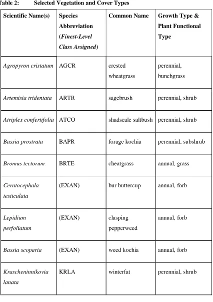
Table 2: Selected Vegetation and Cover Types ... 19
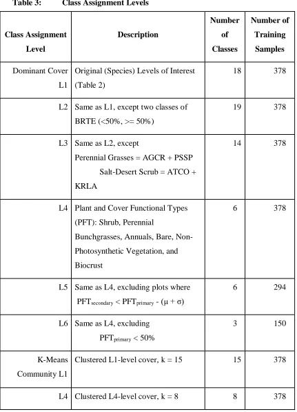
Table 3: Class Assignment Levels ... 24
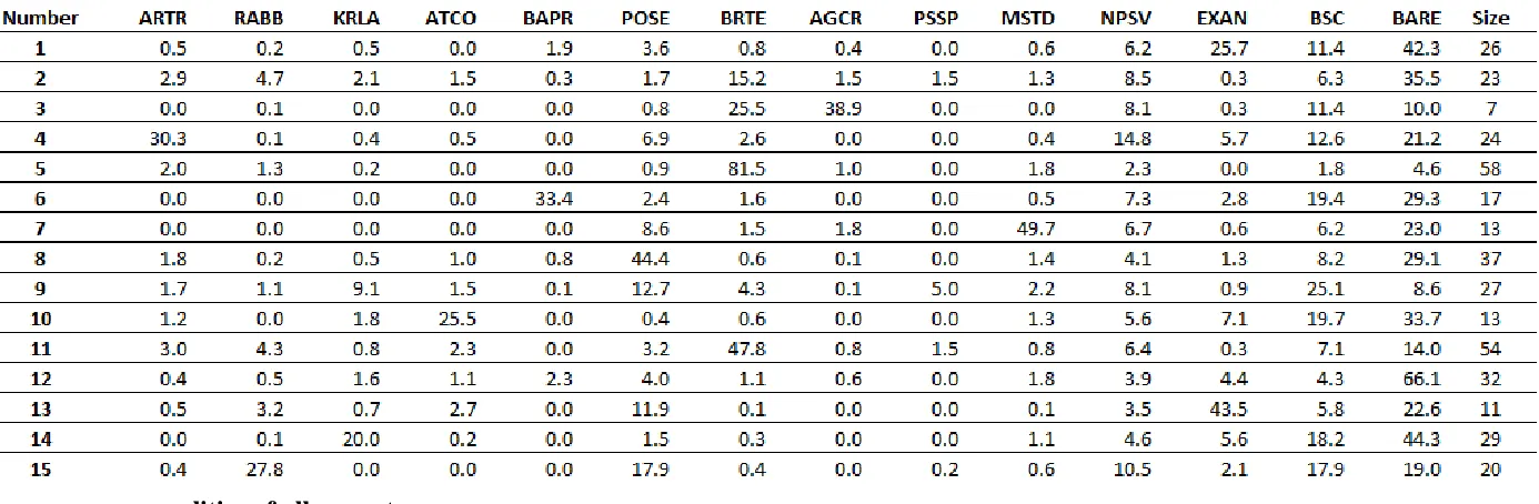
Table 4: K-Means Species-Level (L1) Cluster Mean Centers and Number of Plots per Class. Each cluster is comprised of plots sharing common proportions of one or more cover types, but are not required to have commonalities of all cover types. ... 25
Table 5: K-Means PFT-Level (L4) Cluster Mean Centers and Number of Plots per Class. Each cluster is comprised of plots sharing common proportions of one or more cover types, but are not required to have commonalities of all cover types. ... 27
Table 6: Spectral Indices and Formulas Used in this Study ... 31
Table 7: Cloud Control Dates (year, month, day) ... 32
Table 8: Predictor Variables ... 33
Table 9: Overall Accuracy and Kappa Coefficients for Predictor and Response Variables ... 36
Table 10: Deterministic Confusion Matrix: Community Classes (L1 k = 15) ... 37
Table 11: Cheatgrass Fuzzy (>25% overlap) Confusion Matrix: Community Classes (L1 k = 15) ... 37
Table 12: Sentinel-1 SAR Summary Statistics ... 66
xii
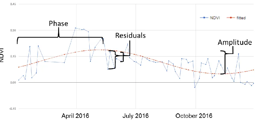
sinusoid fitted to a time series of NDVI values (blue). The phase and amplitude components relate the phenological components of start of growing season and the range of photosynthetic activity as observed from NDVI, and the residuals relate to how well the growing phenology is represented by the sinusoid. ...6 Figure 2: 2 Spectral Characteristics Compared to Landsat 7 and 8. Sentinel-2 has higher spatial resolution than Landsat in addition to several narrow bands in the Red-Edge portion of the electromagnetic spectrum (Bands 5-7, 8a). [NASA, 2015] ... 13 Figure 3: Study Area ... 17 Figure 4: Distributions of Cover Types (species-level). Distributions of each species or cover type used for the L1 and K-means L1 classification schemes, for all field plots. Widths of boxplots represent the number of field plots with the cover type. This figure illustrates that there are very few species that can be found covering more than half of a plot. BRTE (cheatgrass) and BARE (bare, non-biocrust) both have many observations and a large range of percent cover. In comparison, ARTR (sagebrush) has a much smaller percent cover range... 21 Figure 5: Schematic of Field Plot Design ... 22 Figure 6: K-Means Species-Level (L1) Cluster Community Distributions. Each
cluster (1-15) represents a group of field plots sharing similar proportions of cover types. The vertical axis of each cluster represents the density of cover type within the cluster. The horizontal axis represents percent cover of each type. ... 26 Figure 7: K-Means PFT-Level (L4) Cluster Community Distributions. Each cluster
(1-8) represents a group of field plots sharing similar proportions of cover types. The vertical axis of each cluster represents the density of cover type within the cluster. The horizontal axis represents percent cover of each type. ... 28 Figure 8: Example Illustration of Percent Overlap in BRTE Distributions. This
xiii
Figure 9: NDVI Harmonic Coefficients. Image a) illustrates the three predictor coefficients (b-d, normalized to 1) in Saturation-Hue-Value, respectively. The background of a) shows the number of Sentinel-2 scenes used for the harmonics, where overlap in delivered MGRS tiles and the data-take (diagonal) artefacts are apparent. The RMSE band b) contains the majority of calculation artefacts. ... 41 Figure 10: Precipitation and B8A (Red Edge 865 nm) for a Sagebrush Plot
(-116.3656650619256, 43.23953563635724), Vertical lines and arrows illustrate the correlated lag concept. ... 68 Figure 11: Gini-ranked Variable Importance ... 69 Figure 12: Imputed Biological Soil Crust Percent Cover in the Morley Nelson Snake
River Birds of Prey, 2016 ... 71 Figure 13: Predicted vs. Observed Biological Soil Crust Cover, R-Squared 0.74 ... 72 Figure A.1: Imputed Bare Cover in the Morley Nelson Snake River Birds of Prey,
2016 ... 97 Figure A.2: Predicted vs. Observed Bare Cover ... 97 Figure A.3: Bare Cover (red) vs. Biocrust Cover (blue) in the Morley Nelson Snake
xiv B1 Band 1 (also Bands 2-12) BOA Bottom of Atmosphere BOP Birds of Prey
BSC Biological Soil Crust BSS Between Sum-of-Squares
CHIRPS Climate Hazards Group InfraRed Precipitation with Station data
EM Endmembers
ESA European Space Agency GEE Google Earth Engine GPS Global Positioning System
GSM General Soil Map (of the United States)
HA Harmonic Analysis
HC Harmonic Coefficient IDANG Idaho Army National Guard IQR Inner-Quartile Range MAE Mean Absolute Error
MC Monthly Composite
xv MPP Mixed-Pixel Problem
NASA National Aeronautics and Space Administration NDVI Normalized Difference Vegetation Index NIR Near Infrared
OA Overall Accuracy
OCTC Orchard Combat Training Center PFT Plant Functional Type
RF Random Forest
RMSE Root-Mean-Squared Error
RTK GPS Real-Time-Kinematic Global Positioning System
S1 Sentinel-1
S2 Sentinel-2
SMAP Soil Moisture Active Passive
SP SamplePoint
SPOT Satellite Pour l’Observation de la Terre SSURGO Soil Survey Geographic Database STATSGO2 State Soil Geographic dataset TOA Top of Atmosphere
TLA Three-Letter Acronym TSS Total Sum-of-Squares
CHAPTER ONE: TIME-SERIES, SENTINEL-2, VEGETATION MAPS IN SEMI-ARID ECOSYSTEMS
Abstract
As a modification of the common phrase “garbage in, gospel out” conveys, the success of a remote sensing vegetation classification relies not on complex or seemingly magical statistical and physical models using neural networks in abstract ‘feature space’, but rather on the quality of its input data. Semi-arid ecosystems are no exception; they contain very few types of land cover that can be found in patch sizes larger than the pixel with which they are represented - even at 10-meter scale pixels. Creating a vegetation map that assigns a single species or plant functional type to each pixel has limitations and may provide as little information as “this category is here in some proportion, likely”. But how can field observations of nature be translated into a form compatible with scientific investigation? Is the output data meaningful for land managers or ecosystem modelers? Using robust field data of vegetative cover combined with a time-series of
high-resolution multispectral imaging, this paper examines the relationship between
Background and Introduction
Semi-Arid Ecosystems & Remote Sensing Thereof
Dryland environments occupy nearly 40% of Earth’s terrestrial surface
[Millennium Ecosystem Assessment, 2005] and are increasingly affected by changes in climate and land use (Li et al. 2015). While our understanding of their function and global impact is enough to know that they are important, our knowledge falls short of adequate [Millennium Ecosystem Assessment, 2005]. It would be difficult to understate the importance of dryland environments. Approximately 38% of the global population inhabits drylands, of which 250 million people in the developing world are directly impacted by degradation of such environments [Reynolds et al., 2007]. Semi-arid
ecosystems have been observed to be a driving factor in the interannual variability of the global carbon cycle [Poulter et al., 2014]. Dynamics of such ecosystems are reflective of changes in climate (interannually and as part of larger trends), vegetation communities (as a result of invasive species), land use (from many past uses and management approaches), and fire (as a result of the previous three).
Understanding the interactions between climatic changes and vegetative response is therefore important at the global scale. At regional scales, understanding the dynamics of semi-arid vegetation community composition is important for fire risk, mitigation, and restoration [Shinneman et al., 2015], and for management efforts to balance multiple uses [Knick and Rotenberry, 1997].
in relation to soil background, and high seasonal variability. These challenges are often met with high spectral and spatial resolution (as in airborne hyperspectral imaging), or high temporal resolution (as in MODIS or AVHRR time-series). Airborne hyperspectral imaging is expensive to collect and requires significant data processing, and consequently is not collected many times over the same area. While MODIS imagery is collected every one to two days in 36 spectral bands, the spatial resolution (250m-1.1km) is not
commensurate with the scale of semi-arid vegetation (classically described as ‘patchwork’, varying through the landscape on the scale of 10s of meters or less).
It would be unfair to characterize these two approaches as the only options. The Landsat, SPOT, and RapidEye satellite constellations offer good compromises between temporal, spectral, and spatial resolution. They have all been used successfully to map semi-arid vegetation by leveraging their strengths, sometimes in concert with other platforms. New platforms such as the ESA’s Sentinel-2 satellites offer advances in optical remote sensing beneficial to vegetation mapping in dryland ecosystems, such as increased spatial and temporal resolution.
Phenology and Time-Series
and when such occur in a growing season [Braget, 2017]. The second - phenology - examines temporal signals by matching observed with reference temporal signals, or comparing fitted mathematical curves (“reconstructed time-series”) to the signals [Zhou et al., 2016].
Phenometric time-series use metrics such as the beginning and end of a growing season and the date of maximal photosynthetic activity (observed from spectral indices such as NDVI) to preserve some temporal component of remote sensing data. In fact, retaining the maximum value of a spectral index can be sufficient for classification (such as in the Maximum-Value Composite procedure, Holben 1986). However, such
approaches rely on selecting the appropriate time window to capture maximal variation in vegetative responses, while being sufficiently large to reduce atmospheric and anomalous values, and small enough to minimize the likelihood that neighboring pixels are collected at increasingly different times [Vancutsem et al., 2007; Zhou et al., 2016]. Additionally, the relative and absolute thresholds used to determine the beginning and end of the growing seasons can be difficult to establish (e.g. what point of the curve is the ‘start’), and the frequency component of vegetative responses are not captured [Huesca et al., 2015]. This is problematic for many types of semi-arid vegetation, which respond strongly to precipitation events. However, this methodology can be applied with
platforms that have higher spatial resolution but generally less temporal resolution (such as Landsat).
as MODIS which trade high revisit frequency with spatial and spectral resolution [Iiames, 2010]. Other methods relate the temporal resolution of MODIS with the spatial and spectral qualities of Landsat [Gallagher, 2018]. Yet others ‘reconstruct’ time-series data by filling gaps between observations or by fitting mathematical functions to the
observations [Zhou et al., 2016]. Such temporal data can therefore leverage methods that examine vegetation’s’ ‘signal’ more directly in the frequency domain.
The Mixed Pixel Problem and Hard, Soft, and Fuzzy Classifications
The mixed-pixel problem (MPP) is well known in remote sensing classifications. For the purposes of this paper, a mixed-pixel is a pixel that represents some proportion of two or more ‘classes’. The notion of a ‘class’ that can be represented with a rectangular shape is the root of this problem; a pixel is assigned to a single class such as ‘tree’ when it is only ‘mostly tree’ or more specifically, the remotely-sensed signal is more consistent with ‘tree’ than it is other classes. This belies the issue that the observed signal from training locations called ‘tree’ are assumed to a pure signal of ‘tree’, when in fact some may be 60% tree and others 85%, and some may have a background of dark soil as the remaining portion, and others with a verdant meadow as an understory. Should a pixel containing mostly ‘tree’ have enough of a different composition to fall outside of the distribution of the training ‘tree’ pixels, the classification may decide that it would be better called ‘shrub’, or perhaps ‘building’. The classifier may not have any clear choice, since it likely has no training pixels that match the pixel in question. Or, should the pixel contain 50% tree and 50% building, the resulting signal may happen to be more closely aligned with signals of ‘shrub’ pixels than those of either the ‘tree’ or ‘building’ classes. These are the classification issues that can arise from the mixed-pixel problem
[Gebbinck, 1998].
may describe the plot as 40% soil and 60% shrub, but the observed signal may be closer to the sum of a plot of 60% soil and 40% shrub - a complete change of class. Second, the signal of one cover type of interest may not be adequately observed due to the portion in which it naturally occurs, or at the date in which the image is collected. Even if a short, delicate bunchgrass is the dominant ‘class’, it may be difficult to observe its signal apart from the soil. This does not necessarily cause confusion if the signal is representative (i.e. ‘bare’ as a proxy for the bunchgrass), but should ‘bare’ be its own class of interest then significant under classification may occur (errors of omission).
There are several remote sensing approaches designed to address the mixed-pixel problem. The first is to simply acquire imagery of higher spatial resolution. A similar scale allows the pixel to better represent the subjects of interest [Fraser et al., 2014]. However, this can introduce ‘new’ spectral classes that were not previously observable at a coarse scale [Campbell and Wynne, 2011], and can result in a similar classification outcome - this time just at a finer spatial scale.
proportional composition. This has been done by assessing confidence levels per class, but is still dependent in some fashion on a single class per pixel (i.e. 100% confidence).
Another solution uses very high spectral resolution data to ‘unmix’ pixels. More comprehensive spectral signatures, especially at a high spatial resolution (≈1m) allow subtle distinctions between pixels to be observed. Known spectral endmembers (‘pure’ pixels, either from known locations in the images, or a reference signal) can then inform unmixing of the pixel into its likely constituents. This process has been used with remarkable success, even in shrub-steppe environments [Poley, 2017].
the advantage of accounting for physical interactions with photons at the canopy scale, and seeks to relate such insight into more accurate classifications. However, it does little to address the MPP directly.
Yet other approaches leverage the changes in a pixel over time as in phenology (see above section). This additional order of dimensionality enables greater distinction between pixels, and potentially the ability to group pixels that are ‘more similar’ over time. Huesca et al. [2015] apply the “Optical Types” framework in this way. This approach effectively links Optical Types with temporal dynamics. Their concluding remark: “Thus, exploration of temporal dynamics presents a promising opportunity to further explore vegetation composition within mixed pixels.”
The majority of approaches outlined so far have sought to decompose the signal into its constituent parts (fuzzy membership, spectral unmixing), collect higher resolution imagery (spatial, spectral, or temporal) with the hopes of discerning better between classes, or to justify confusion errors after classification. Few, if any, have attempted to perform classification on pixels assumed to be mixed (soft) when they are input into the classification model.
Sentinel-2
The European Space Agency's Sentinel-2 constellation (opposing twin satellites, A and B) is directed at monitoring the land surface and coastal waters with
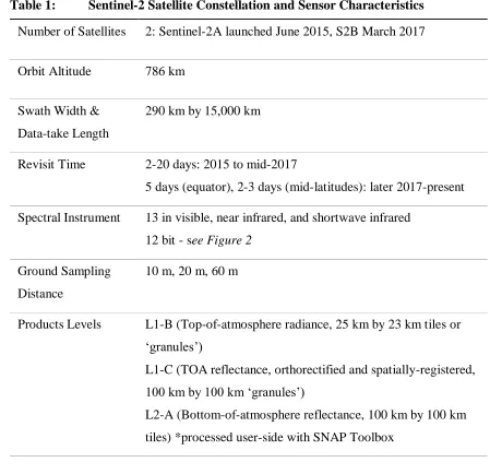
Table 1: Sentinel-2 Satellite Constellation and Sensor Characteristics
Number of Satellites 2: Sentinel-2A launched June 2015, S2B March 2017
Orbit Altitude 786 km
Swath Width & Data-take Length
290 km by 15,000 km
Revisit Time 2-20 days: 2015 to mid-2017
5 days (equator), 2-3 days (mid-latitudes): later 2017-present Spectral Instrument 13 in visible, near infrared, and shortwave infrared
12 bit - see Figure 2 Ground Sampling
Distance
10 m, 20 m, 60 m
Products Levels L1-B (Top-of-atmosphere radiance, 25 km by 23 km tiles or ‘granules’)
L1-C (TOA reflectance, orthorectified and spatially-registered, 100 km by 100 km ‘granules’)
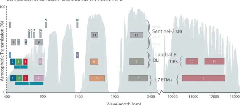
Figure 2: Sentinel-2 Spectral Characteristics Compared to Landsat 7 and 8. Sentinel-2 has higher spatial resolution than Landsat in addition to several narrow bands in the Red-Edge portion of the electromagnetic spectrum (Bands 5-7, 8a).
[NASA, 2015]
The increased spatial resolution (10-20 m, compared to 30-60 m) is markedly closer to scales important for land management and planning decisions [Cihlar, 2000; Franklin and Wulder, 2002], and closer to the scale of human influences [Wulder et al., 2012]. Higher spatial resolution means more representative pixels (i.e. less mixed pixels), especially in areas where the vegetative cover is patchy or highly variable. Monitoring the change in position of an ecotone, for example, is difficult if the footprint of the pixel straddles the entire transition. Other less immediately-recognized benefits of higher spatial resolution pixels are better cloud screening (as clouds are less-often included within a pixel), and better image coregistration and georeferencing.
way that information from these platforms are often used together. While S2’s blue, green, red, and near-infrared bands were designed to capture similar wavelengths as Landsat 7 and 8 (Figure 2), the small differences in spectral responses requires bandpass adjustment in order to be used together [Claverie and Masek, 2016]. The ESA delivers S2 scenes at Level-1C, which includes top-of-atmosphere (TOA) reflectance in cartographic geometries which are registered to be within 3, 6, or 18 m per pixel for the 10, 20, and 60 m bands, respectively (Table 1: Sentiel-2 Characteristics). While ESA’s freely-available SNAP toolbox can perform atmospheric corrections to bottom-of-atmosphere (BOA) reflectance (Level-2A), it still requires that the user download and process each scene on a personal computer [Baillarin et al., 2012]. Using TOA values for temporal comparisons can be problematic as a result of changing atmospheric conditions. Unfortunately, several of the important spectral bands are sensitive to atmospheric interferences; for example TOA NDVI is lower than BOA NDVI [Beck et al., 2006].
Imagery from 2016 is additionally challenging. Sentinel-2B was not launched until March 2017, so the full temporal resolution was not realized in 2016. While the temporal resolution of a single S2 satellite (A or B) would be ten days, it can vary from two to twelve as the orbit of Sentinel-2A was modified several times. Spatial
misalignment of delivered scenes has also been an issue, but ESA have generally
inside one MGRS tile are delivered with the label of the tile but are only a sliver of the image. The processing baseline for imagery has also been updated several times, as well as some of the metadata format. These issues complicate spatial and temporal
compositing of Sentinel-2 imagery. Figure 9 illustrates this issue. Research Question
Remote sensing of vegetation in semi-arid ecosystems and drylands is inherently challenging. Phenology in these ecosystems is highly dynamic both in response to weather and climatic changes, and through the growing season. Fractional vegetative cover is low and community composition is heterogeneous at scales from tens to hundreds of meters. These difficulties lead to two questions: 1) are a cohort of spectral predictors at regular time intervals better than a generalized phenology curve, or are a few ‘snapshots’ equivalent? and 2) what is a meaningful way to characterize vegetation on a scale commensurate with remote sensing imagery?
I investigate the first question by comparing classification accuracies using imagery from discrete time-series (monthly) composites, sinusoidal approximations of time-series data (“harmonic” models), and both in concert. I contrast these results with a control set of predictor variables consisting of all dates of cloud-free imagery covering the study area. Keeping the spatial resolution the same (10 meter pixels) and using the same spectral predictors with each approach highlights how the differences in temporal representation correspond to classification accuracies.
(irrespective of majority cover/greater than 50%) at several hierarchical levels from species-level to Plant Functional Types (PFTs). I also explore the effects of barriers to class membership (majority cover, and without strong co-dominant cover) on
classification accuracy. Next, I use a clustering algorithm to determine ecologically meaningful (‘soft’) classes. Finally, I propose a method to evaluate classification accuracies of the soft classes that reserves interpretation for the vegetation map user.
Taken together, insights from these questions inform remote sensing
classifications of semi-arid vegetation, and preserves interpretation for land management and scientific inquiry.
Materials and Methods
Study Area
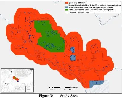
salt-desert shrubs (primarily members of the Chenopodioideae subfamily), and bunchgrasses (Poa secunda, Pseudoroegneria spicata, and Agropyron cristatum).
Figure 3: Study Area
history of changing land uses and practices, the BOP is a ‘patchwork’ of many different vegetative communities. Balancing the current uses of the study area requires managing agencies and stakeholders to be informed of yearly changes in vegetative cover, impacts of rangeland fires, and how restoration and remediation efforts are progressing. To this end, increasing the accuracy of vegetation cover data and frequency of its creation is propitious.
Field and Training Data
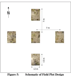
Field data plots used in this study (n = 378) were collected during March-August 2016. Field data plots were selected in the field as homogenous communities of each vegetation and land cover type (Table 2: Selected Vegetation and Cover Types), and representative of different community combinations and variations among spatial gradients. A field survey was conducted for each plot, and five nadir-pointing images were taken approximately two meters above the ground surface using a 16-megapixel all-weather camera (Nikon COOLPIX AW120). A RTK GPS recorded the imager’s location simultaneously (Figure 5: Field Plot Design). Vegetation and groundcover were
Table 2: Selected Vegetation and Cover Types
Scientific Name(s) Species
Abbreviation
(Finest-Level
Class Assigned)
Common Name Growth Type &
Plant Functional
Type
Agropyron cristatum AGCR crested wheatgrass
perennial, bunchgrass
Artemisia tridentata ARTR sagebrush perennial, shrub
Atriplex confertifolia ATCO shadscale saltbush perennial, shrub
Bassia prostrata BAPR forage kochia perennial, subshrub
Bromus tectorum BRTE cheatgrass annual, grass
Ceratocephala testiculata
(EXAN) bur buttercup annual, forb
Lepidium perfoliatum
(EXAN) clasping
pepperweed
annual, forb
Bassia scoparia (EXAN) weed kochia annual, forb
Krascheninnikovia lanata
Descurainia spp., Sisymbirum ssp.
(MSTD) mustards annual, forb
Poa secunda POSE Sandberg’s
bluegrass
annual, bunchgrass
Pseudoroegneria spicata
PSSP bluebunch
wheatgrass
annual, bunchgrass
Chrysothamnus nauseosus
(RABB) gray rabbitbrush perennial, shrub
Chrysothamnus viscidiflorus
(RABB) green rabbitbrush perennial, shrub
- (BARE) bare ground n/a, bare
- (BSC) biological soil
crusts
bacteria, moss, and lichen; groundcover
- (NPSV)
non-photosynthetic vegetation
Figure 5: Schematic of Field Plot Design
Assigning Hierarchical Levels of Dominant Cover
splitting classes with many members into smaller classes (i.e. BRTE, Level 2), up to the level of Plant Functional Types (PFTs, Level 4). The second philosophy sought to increase the distinction of each PFT class by imposing criteria for membership (Levels 4-6). Table 3 lists the differences between each dominant cover level.
Assigning Ecological Classes Using K-Means Clustering
Table 3: Class Assignment Levels Class Assignment Level Description Number of Classes Number of Training Samples Dominant Cover L1
Original (Species) Levels of Interest (Table 2)
18 378
L2 Same as L1, except two classes of BRTE (<50%, >= 50%)
19 378
L3 Same as L2, except
Perennial Grasses = AGCR + PSSP Salt-Desert Scrub = ATCO + KRLA
14 378
L4 Plant and Cover Functional Types (PFT): Shrub, Perennial
Bunchgrasses, Annuals, Bare, Non-Photosynthetic Vegetation, and Biocrust
6 378
L5 Same as L4, excluding plots where PFTsecondary < PFTprimary - (μ + σ)
6 294
L6 Same as L4, excluding PFTprimary < 50%
3 150
K-Means Community L1
Clustered L1-level cover, k = 15 15 378
25
Table 4: K-Means Species-Level (L1) Cluster Mean Centers and Number of Plots per Class. Each cluster is comprised of plots sharing common proportions of one or more cover types, but are not required to have
Table 5: K-Means PFT-Level (L4) Cluster Mean Centers and Number of Plots per Class. Each cluster is comprised of plots sharing common proportions of one or more cover types, but are not required to have commonalities of all cover types.
Imagery and Predictor Variables
Imagery Selection & Preprocessing
Level-1C Sentinel-2 imagery covering the study area from 01 January 2016 to 28 December 2016 were selected to span the growing season corresponding to the field data collection. Images were preliminarily filtered to remove small image footprints (ESA processing artefacts as discussed in Background: Sentinel-2), images that failed radiometric or general quality control, and scenes with greater than 50% cloud cover (from metadata, for speed of processing). The resulting image collection was comprised of 117 images.
Cloud & Shadow Masking
Cloud and shadow masking algorithms were applied to each image using tiered thresholds. This method is a modification of a community-developed algorithm
cloud masking algorithm. The January mosaic was visually inspected to ensure that no significant clouds or shadows were visible in the final mosaicked scene. The February mosaic was discarded due to the excessive proportion of masked pixels, which resulted in all field observations having null values for this time.
Spectral Indices & Predictor Variables
Table 6: Spectral Indices and Formulas Used in this Study
Index or Ratio Abbreviation Formula
Anthocyanin Reflectance
Index ARI (
1 𝐵3) − (
1 𝐵5)
Canopy Chlorophyll
Content Index CCCI
𝐵8𝐴 − 𝐵7 𝐵8𝐴 + 𝐵7 𝐵8𝐴 − 𝐵4 𝐵8𝐴 + 𝐵4
Enhanced Vegetation Index EVI 2.5 ∗ ( 𝐵8 − 𝐵4
𝐵8 + (6 ∗ 𝐵4) − (7.5 ∗ 𝐵2) + 1)
Inverted Red-Edge
Chlorophyll Index IRECI
𝐵7 − 𝐵4 𝐵5/𝐵6
Normalized Difference
Near Infrared Red-Edge NDMI
𝐵8𝐴 − 𝐵11 𝐵8𝐴 + 𝐵11
Normalized Difference
Vegetation Index NDVI
𝐵8 − 𝐵4 𝐵8 + 𝐵4
Sentiel-2 Red-Edge
Position S2REP 0.705 + 0.035 ∗
(𝐵7 + 𝐵4)/2 − 𝐵5 𝐵6 − 𝐵5
Soil Composition Index SCI 𝐵11 − 𝐵8
𝐵11 + 𝐵8
residuals of the harmonic calculation were used as predictors. Figure 1 illustrates the metrics derived from each harmonic model, calculated for each pixel.
As a control for issues caused by cloud and shadow masking, temporal
compositing, and harmonic coefficient calculations, S2 collections with little to no cloud cover were also evaluated for predictive ability using the same bands and spectral indices as the 30-day composites. Eight dates had imagery covering the entire study area where all but one tile had less than six percent cloud cover. Table 7 lists dates and cloud cover for these images. Table 8 summarizes predictor variables.
Table 7: Cloud Control Dates (year, month, day)
Date Used
Table 8: Predictor Variables
Predictor Data Sets Number of Variables Description
Cloud Control: Bands and Spectral Indices
184
(8 observations of 23 variables)
All low-cloud imagery with complete coverage of study area of same-day; Bands and spectral indices as predictors
Monthly (30-Day) Composites: Bands and Spectral Indices
253
(11* observations of 23 variables)
Prefiltered images, cloud and shadow masked, composited based on pixel quality every 30 days Same as Cloud Control
Harmonic Coefficients 69
(3 curve metrics of 23 variables)
Prefiltered, masked, with original temporal
component;
Phase, amplitude, and RMSE as predictors
Monthly Composites + Harmonic Coefficients
322 (253 + 69)
Classification & Random Forest Model
The random forest (RF) classifier was chosen to evaluate the different predictor and response variable combinations due to the high dimensionality and multicollinearity of the predictor variables, and its insensitivity to overfitting [Breiman, 2001; Belgiu and Dragut, 2016]. The RF classifier can handle unbalanced data [Pal, 2005], which is important for the field data in this study, as some classes of interest are relatively under-represented in comparison with others (e.g. number of shadscale plots verses cheatgrass plots). It is also able to handle missing values when imputing the classification, which is advantageous for portions of the predictor data that contain masked areas after
mosaicking. As implemented in GEE, training data must be free of missing values to grow a RF model.
Field data points were buffered using a 10 m radius, and the mean value of the intersected pixels in each band were extracted as the predictor variables for the RF model. The RF model was implemented in Google Earth Engine using 500 trees and out-of-bag internal sampling, with a random seed value of zero. Data was divided into training data (67%) and validation data (33%) using a random number. The validation data set was used to calculate a confusion matrix at each level of predictor imagery. Accuracy Assessment
Accuracy assessment was performed for each of the classification schemes (L1-L6) against each predictor set by calculating the overall accuracy of a deterministic confusion matrix generated through the internal OOB validation of RF. Kappa
Accuracy of the k-means vegetation classification schemes were assessed as above, with the addition of a matrix representing “fuzzy” confusion for select classes. Determining acceptable fuzzy confusion between ecotype classes was calculated for each of the cover types by examining the percent of overlap of the density distributions per class. If the mean value of each cover type was greater than 25%, the intersection of each distribution was summed. This overlap threshold was then applied, and the combination of clusters was flagged as an acceptable fuzzy confusion for that class if the overlapping percentage exceeded the threshold. Additional overlap thresholds were examined (75% and 50%) but are not presented here.
Results
Table 9: Overall Accuracy and Kappa Coefficients for Predictor and Response Variables
As Table 9 illustrates, results show that overall accuracy (OA) for dominant cover classes (L1-L4) increased with increasing levels of aggregation (L1-L4). Similarly, more selective criteria generally increased levels of overall accuracy (L4-L6). The mean increase from the species-level class (L1) to the PFT (L4) was 8.25%, and the mean increase from PFT (L4) to stringent-membership PFT (L6) was 25%. Kappa values followed similar patterns, and illustrate that the certainty of each classification improves with increasingly broad classes.
The results of the k-means-clustered data were similar with several notable exceptions. The control, MC, and HC+MC predictors returned roughly equivalent OA and K, while OA and K for the HC model alone using L1 k-means clusters was lower (Table 9). The k-means classes based on the coarser aggregation (L4 PFT) had slightly lower accuracies than the k-means classes determined from the finer-level cover classes (L1). Table 11 presents an example fuzzy classification with a focus on BRTE cover; Figure 8 illustrates one overlap distribution between two classes.
Overall
Accuracy Kappa OA K OA K OA K
(Species) L1 0.58 0.40 0.59 0.42 0.60 0.44 0.60 0.44
L2 0.50 0.32 0.53 0.37 0.54 0.40 0.53 0.37
L3 0.53 0.36 0.55 0.40 0.56 0.41 0.55 0.40
(PFT) L4 0.62 0.43 0.66 0.50 0.66 0.49 0.68 0.52
L5 0.65 0.45 0.71 0.54 0.72 0.57 0.72 0.56
L6 0.86 0.69 0.89 0.77 0.89 0.77 0.88 0.74 k -means
L1 k = 15 0.40 0.33 0.48 0.42 0.49 0.43 0.50 0.45
L4 k = 8 0.47 0.37 0.52 0.44 0.55 0.47 0.52 0.44 PREDICTOR VARIABLES
Table 10: Deterministic Confusion Matrix: Community Classes (L1 k = 15)
Table 11: Cheatgrass Fuzzy (>25% overlap) Confusion Matrix: Community Classes (L1 k = 15)
Consumers accuracy:
1 2 3 4 5 6 7 8 9 10 11 12 13 14 15 SUM
1 8 0 0 1 0 2 1 1 1 0 0 6 3 2 1 26 0.31
2 0 5 0 0 0 1 0 0 1 0 9 3 0 0 1 20 0.25
3 0 0 0 0 0 0 0 0 1 0 4 0 0 1 0 6 0.00
4 0 0 0 10 3 0 0 1 1 0 6 0 1 0 1 23 0.43
5 1 0 0 0 45 0 0 1 0 0 7 0 0 1 2 57 0.79
6 2 0 0 1 0 7 0 0 0 0 0 4 0 0 3 17 0.41
7 1 0 0 0 2 0 5 1 0 0 1 2 0 0 1 13 0.38
8 1 1 0 0 1 0 0 17 2 0 5 5 0 1 2 35 0.49
9 1 0 0 1 2 0 0 4 5 2 5 0 0 3 3 26 0.19
10 0 0 0 1 0 0 0 0 3 5 0 0 0 4 0 13 0.38
11 0 4 0 4 13 1 0 5 0 0 24 1 0 0 0 52 0.46
12 5 2 0 0 0 0 0 1 0 0 0 21 0 3 0 32 0.66
13 3 0 0 2 0 0 0 1 0 0 0 0 2 0 1 9 0.22
14 2 1 0 0 1 0 0 0 2 2 0 5 0 16 0 29 0.55
15 0 0 0 1 0 0 0 3 0 0 2 0 0 0 14 20 0.70
SUM 24 13 0 21 67 11 6 35 16 9 63 47 6 31 29 Correct: 184
0.33 0.38 - 0.48 0.67 0.64 0.83 0.49 0.31 0.56 0.38 0.45 0.33 0.52 0.48 Total: 378
0.49 C la ssi fi e d Pl o ts Reference Plots Overall Accuracy: Producers accuracy: CLASS Consumers accuracy:
1 2 3 4 5 6 7 8 9 10 11 12 13 14 15 SUM
1 8 0 0 1 0 2 1 1 1 0 0 6 3 2 1 26 0.31
2 0 5 0 0 0 1 0 0 1 0 9 3 0 0 1 20 0.25
3 0 0 0 0 0 0 0 0 1 0 4 0 0 1 0 6 0.00
4 0 0 0 10 3 0 0 1 1 0 6 0 1 0 1 23 0.43
5 1 0 0 0 45 0 0 1 0 0 7 0 0 1 2 57 0.79
6 2 0 0 1 0 7 0 0 0 0 0 4 0 0 3 17 0.41
7 1 0 0 0 2 0 5 1 0 0 1 2 0 0 1 13 0.38
8 1 1 0 0 1 0 0 17 2 0 5 5 0 1 2 35 0.49
9 1 0 0 1 2 0 0 4 5 2 5 0 0 3 3 26 0.19
10 0 0 0 1 0 0 0 0 3 5 0 0 0 4 0 13 0.38
11 0 4 0 4 13 1 0 5 0 0 24 1 0 0 0 52 0.46
12 5 2 0 0 0 0 0 1 0 0 0 21 0 3 0 32 0.66
13 3 0 0 2 0 0 0 1 0 0 0 0 2 0 1 9 0.22
14 2 1 0 0 1 0 0 0 2 2 0 5 0 16 0 29 0.55
15 0 0 0 1 0 0 0 3 0 0 2 0 0 0 14 20 0.70
SUM 24 13 0 21 67 11 6 35 16 9 63 47 6 31 29 Correct: 184
0.33 0.38 - 0.48 0.67 0.64 0.83 0.49 0.31 0.56 0.38 0.45 0.33 0.52 0.48 Total: 378
0.49 82
Fuzzy Accuracy: 0.70
Correct Points at Overlap >25% BRTE Note: outlined boxes denote classes with >25%
overlap in BRTE distributions
Figure 8: Example Illustration of Percent Overlap in BRTE Distributions. This figure illustrates that two different classes (2 & 3 in this example) may have similar distributions of a particular cover type. Therefore, if BRTE is the species of interest to the map user, confusion between these classes is acceptable. This commutability forms the basis for ‘fuzzy’ confusion. The level of acceptable overlap is additionally determined by the map user.
Discussion
A faithful representation of pixel-scale vegetative and land cover can be created without using advanced unmixing techniques of hyperspectral data. Vegetation
classification using ecologically-meaningful communities as classes (as discussed in Assigning Ecological Classes and in Figures 6 and 7), combined with user-specific fuzzy confusion matrices (Tables 4 and 5) is a better approach than classifications using
majority cover as classes and a single deterministic error matrix. This new method requires robust field observations and inclusion of some temporal remote sensing data, but the results are worthwhile for two reasons. First, community-classes are a more faithful representation of vegetative communities in semi-arid and dryland ecosystems, since very few species or types exist as 100% cover at the 10-meter-by-10-meter pixel scale. Second, the overlapping distributions of each species or type between clusters allows for fuzzy confusion between classes based on the question at hand. Although this approach requires more engagement from the map user, it enables greater flexibility in how the classification is used and most likely increases the probability that the
information in the map is used to inform management or planning decisions. Predictor Variable Importance
representing areas of the same cover type. The 30-day window was chosen for this study due to the inconsistent nature of Sentinel-2A’s 2016 orbit pattern (revisit period ranges from 2-20 days). Studies using 2018 data will be able to take full advantage of the consistent 5-day revisit period, and can therefore choose smaller compositing windows.
The comparable success of the control dates may also be due to a fortuitous eight particular days (Table 7) that happened to capture enough differences in phenology, and therefore this result is not transferrable to other study areas or years. Iteratively removing several of the cloud-free control dates and observing decreases in accuracy will provide further insight to the influence of particular dates, or number of temporal observations needed. Increasing the monthly compositing window to 60 days and observing the change in classification accuracies could also elucidate the effects of compositing.
Harmonic Model Performance
The harmonic models alone have roughly equivalent overall accuracies to the MC, HC+MC, and control sets. If the volume of data is an issue (e.g. outside of GEE or similar cloud computing environment), the significance of comparable accuracies is important: the HC predictors were able to classify nearly as well as using 34% of the data size of the MC predictors (15.1 GB vs 44.3 GB).
The lower kappa values of the HC models indicate a higher portion of
classification accuracy is attributable to chance. Although cursory exploration indicated that the RMSE value (‘goodness-of-fit’ of harmonic sinusoid to the data) was equivalent in predictive ability to the amplitude and phase, it could be related to some of the
Harmonic NDVI Separate Bands). The overlapping areas of the imagery are caused either by delivering the same pixel values with the two adjacent tiles, or the same area is
imaged a day apart (the diagonal stripe from NNE to SSW), or both. This mosaicking issue requires further scrutiny.
Selecting Categorical Levels of Response Variables Is Important Plant Functional Types More Reliable than Species Levels
The results exploring measures of dominant cover class distinctions demonstrate that aggregation at the PFT level are more accurately classified compared to species-level class assignments, and that the threshold of class membership significantly influences classification outcome.
phenologies such as annuals and perennial grasses. This level had the highest overall accuracies due to these broader similarities.
Stringent Requirements for Class Membership Increases Accuracy, at a Cost The largest increase in overall classification accuracy was observed in the differences between the dominant PFT plots as training data (L4) compared with only selecting plots containing more than 50% of the PFT cover (L6). Selecting training data from plots whose second/codominant PFT was significantly less than the
primary/dominant PFT (PFT2 < PFT1 - (μ + σ); L5) increased overall classification accuracy slightly between all predictor variables. This is analogous to selecting endmembers (EMs) in the process of spectral unmixing.
However, it is more likely that the increase in overall accuracies (as well as kappa coefficients) are attributable to a reduction in the number of classes, as higher standards for membership begin to diverge from the realities of semi-arid vegetative ecotypes. For example, only three classes remain after imposing thresholds for L6: shrub (n = 4), bare (n = 50), and annuals (n = 96). Such a classification could not be used for land
management purposes even if these were the only classes of interest; all of the shrub plots were classified as annuals. Should it have been accurate, errors of omission would likely be greater for shrubs since the threshold for PFT class membership (> 50% cover) is not representative of most shrub communities in the study area.
Soft and Fuzzy Classification Schemes
dimensions (i.e. greater numbers of variables) better distinguish between classes. Thus, there are more ways to distinguish between k-means clusters generated at the species-level than at the PFT-species-level. Pursuant to the overarching goal of producing a
representative vegetation map, this is a desirable corollary: k-means clusters at the species level more accurately represent higher-level descriptions of land cover that are of interest for land managers and ecosystem demography modelers.
Further examination of the clusters and their constituent data point to likely sources of this confusion. The Within-Sum-of-Squares (WSS) had a Pearson’s’
Correlation Coefficient of 0.88 compared with the commission errors, and a Pearson’s’ Correlation Coefficient of 0.65 when compared with the omission errors. This indicates that the cluster is sufficiently large to near (or intersect) the distribution of other clusters in one or more dimensions. The L1 k = 15 classes 5, 11, 2, 9, and 4 all had most of the highest WSS. This implies that reducing the number of outliers within each cluster (reducing the WSS) or of the field data would likely reduce confusion between classes. The degree to which this source of error can be reduced likely depends on the ecology of the area in question; vegetative types that exist on a broad continuum and amongst a variety of other community types may require many classes to describe them, or not be able to be separated into distinct groups at all.
Cheatgrass (BRTE) fits this description, and the classes with the highest
confusion errors have high proportions of BRTE as their constituents. This indicates that the pervasive distribution of BRTE is a significant source of confusion. Closer
examination of the distributions of BRTE in each class would better qualify which confusions are acceptable. Repeating this for each class and repeating the ‘focus’ of the confusion matrix would allow for more effective end use. Should the map user be primarily interested in ARTR, referencing the ARTR-based confusion matrix would be more informative. In this way, the imposition of important classes on the data is
Issues, Improvements, and Future Steps Remote Sensing Imagery
Computational limits due to the spatial resolution and study area extent necessitated pre-filtering S2 tiles of excessive cloud cover. Geography outside of the study area but within the same tiles (i.e. the mountains) means that much of a tile can be cloudy, but the portion covering the scene is cloud-free. Methods to calculate the relevant cloudy portion of the study area prior to cloud masking were abandoned due to time constraints, but would potentially allow the inclusion of additional dates.
The predictive ability of the harmonic models will likely improve with increased temporal resolution. Studies from mid-2017 will benefit directly from the increased temporal coverage from Sentinel-2B. Increasing temporal coverage in 2016 could be achieved several ways. Further investment in including all possible S2 scenes (as above) would be one method. Other methods that incorporate other imaging platforms such as the ‘harmonized’ S2 and Landsat data (Claverie et. al 2016), or using MODIS and STARFM to ‘hallucinate’ S2 imagery [Gallagher, 2018] could be used. More
specifically, I could have investigated the threshold for the effects of aberrant (i.e. cloud or shadow) values on the fit of the sinusoid, potentially informing the masking threshold value.
(Bottom-of-Atmosphere reflectance) would likely be a significant improvement
especially for a semi-arid ecosystem where observed reflectance’s can be reduced [Beck et al., 2006].
Including other imagery of different types may increase accuracy of these classifications, as the results of Chapter 2 (below) indicate. For example, including indices from radar (e.g. Sentinel-1) can add information about the physical ‘texture’ or soil moisture of each community type. A time-series of radar data would potentially be able to observe physical changes over a growing season, such as the rapid growth of cheatgrass in the spring or inflorescence of sagebrush later in the fall. Similarly, adding other sources of predictor information such as precipitation, soil type, or land use history (such as grazing and fire) may further improve classification accuracies. In order to preserve the clarity of the research question, such data was omitted for this study.
Training Data
Several aspects of this study can be improved regarding training data. The k-means method to determine community classes allows the data to ‘speak for itself’ but it may be beneficial to examine each member of each class to remove possible outliers. Other more complicated ecosystem demography models may create more ecologically meaningful community classes. An iterative process of determining community classes in tandem with field data collection could create more homogenous cohorts, or inform the proportion and rate of change between two community classes. For example, there may be little gradient between rabbitbrush communities compared with shadscale
communities, but a steady gradient between shadscale and winterfat communities.
percent cover (as in Chapter 2) may lead to a similar outcome with greater degrees of certainty and more easy interpretability, but may not account for the complex interactions of optical wavelengths due to plant canopy structures [Disney, 2016].
Model Development
Although the RF models are able to relate the training data and satellite imagery, a focused effort to examine the relationship between the ‘optical type’ concept proposed by Ustin and Gamon (2010) or similar measurements and the community classes would add surety to the classification model [Cingolani et al., 2008; Huesca et al., 2015]. Other data fusion techniques (such as in Chapter 2) may also improve classification. Further refining of important predictor variables and RF model tuning performed external to GEE but implemented therein has anecdotally been observed to improve model performance in prior iterations of this project, meriting further investigation. Although this study
attempts to preserve interpretability throughout the process, more advanced machine-learning algorithms or neural networks may be able to provide better classification outcomes and more robust metrics of interrelations of classes (measures of fuzziness). Implications
area by approximately 63km SSE and the elevation by an additional 400 meters. This introduced a significant amount of variability in phenology between communities of similar composition, and was therefore excluded.
The soft and fuzzy classification model presented here has the potential to better inform land management and scientific research. It preserves interpretation for the user by the use of fuzzy confusion matrices tailored to the class in question. However, it has been noted that a single map summarizing most land cover information is preferred [Cingolani et al., 2004].
Conclusion
In general terms, this chapter illustrates that the limiting factor of classification accuracy is due to the training data, not the quantity of predictors. While other
approaches using even higher spectral, spatial, or temporal resolutions may not face this same limitation, the Sentinel-2 platform offers a new freely-available compromise of resolutions. This, combined with cloud computing, raise a reminder to evaluate the paradigm of resolution and the scale of subjects.
Corollary to this and specific to semi-arid ecosystems (and those with similar scales of ‘patchiness’) is the possibility to use ecologically-meaningful classes instead of majority-cover classes. Such classes may more closely align with observed remote sensing observations over time, due to the mixed pixel effect and the interaction of light with canopy structure.
equivalent in accuracy, but are an additional level of processing and likely not warranted unless there are limitations in data storage and processing speed.
Input classes are generally better with coarser levels of aggregation (i.e. PFT) and thresholds of membership, but lose levels of ecological meaning in trade. Management needs and research can be better served with more representative classes. For example, there is a key uncertainty in land surface models with the use of PFTs [Hartley et al., 2017]. There are many classification algorithms for relating field observations with remote sensing data, but I posit that more effort should be paid to the methods by which we assign classes to the field data. These approaches should seek to balance the scale of the target subject (e.g. ‘drylands/forest/prairie’ vs. ‘sagebrush/invasive
CHAPTER TWO: REMOTE SENSING OF BIOLOGICAL SOIL CRUST
Abstract
Biological soil crusts (or ‘biocrusts’) are an important but under-studied
component of dryland and semi-arid ecosystems. These ecosystems have large influences on global carbon and nitrogen fluxes, in addition to much of the world’s population health and well-being. Biocrusts are understood to play a significant role in carbon and nitrogen fixation, preserving the health and stability of dryland ecosystems. But this understanding is informed by plant- and plot-scale studies, and refining estimates of global impact remains difficult due to a deficiency of spatial data of biocrust cover. In addition to nutrient fluxes, biocrusts play large roles in soil stability and micronutrient capture, and increase soil moisture by increasing infiltration and decreasing evaporation. Understanding the impacts of these functions on the landscape scale is also hindered by lack of spatial data.
This chapter builds on the methods of Chapter 1, adding more biocrust-specific spectral indices, structural information (from radar), and soil predictor variables. The random forest model is run in regression mode to determine the most significant
Background and Introduction
Semi-Arid Ecosystems and Biocrusts
Scientific papers with study areas in dryland environments appear to be required to point out three things about drylands by the end of their first page: 1) that they occupy nearly 40% of Earth’s terrestrial surface [Millennium Ecosystem Assessment, 2005], 2) that they are fragile and increasingly affected by changes in climate and land use [Li et al., 2015], and 3) that our understanding of their function and global impact is enough to know that they are important but that our knowledge falls short of adequate [Millennium Ecosystem Assessment, 2005; Huang et al., 2016].
Biocrusts are the quintessence of these points. Biocrusts are communities with foundations of cyanobacteria and algae, also containing bacteria, lichens, mosses, and microfauna in varying proportions that live on and within the top few centimeters of soil surfaces. Although biocrusts can be found on all continents [Elbert et al., 2009; Weber et al., 2016] and are one of the most dominant community types on Earth [Weber et al., 2016], their study as an ecosystem component is relatively young – coming of age within the last four decades [Weber et al., 2016, chap.2]. Biocrusts (also called biological soil crust, or occasionally cryptogamic-, cryptobiotic-, microphytic-, mycrobial-, or
microbiotic crust) are most commonly found in the interspaces between vascular plants and under their canopies in arid and semi-arid ecosystems. In some arid ecosystems, they are more than 60% of the land cover [Chen et al., 2005].
than 20 publications in 2000 but over 160 in 2014 (as discussed in Weber et al. 2016). There has been a growing realization that biocrusts play a notable role in global carbon and nitrogen pools and fluxes, but a dearth of spatial understanding is a constraint in quantifying biocrusts’ contribution to natural processes at all scales.
What are Biological Soil Crusts?
Biocrust as an ecological unit is a relatively recent stand-alone field [Belnap and Lange, 2003], and is growing rapidly [Lange and Belnap, 2016, chap.2; Weber et al., 2016, chap.12]. A significant portion of new research is focused on understanding the biological processes and components of these remarkably diverse and highly complex communities. There is also a growing body of scientific literature exploring the ecological functions and impacts of biocrusts from site- to global-scales.
Although demure in appearance, biocrusts play a critical role in arid and semi-arid ecosystems. Filamentous cyanobacteria and algae (along with other structural elements of lichens and bryophytes) form a matrix within the top 1-2 cm of soil [Weber et al., 2016, chap.1]. As this structure develops from several millimeters in thickness, the diversity of organisms increase and the ecological impacts of biocrusts typically increase [Weber et al., 2016, chap.1]. As a physical construction and a biologically-active community, biocrusts influence nearly all transfers of gases, nutrients, and water between the land and atmosphere [Weber et al., 2016, chap.1]. Biocrusts have additional impacts on ecosystem processes, such as carbon and nitrogen fixation in forms beneficial to vascular plant growth [Weber et al., 2016, chap.19].
Although there is a fair amount of uncertainty in recovery rates effectuated by being a young field of study, evidence of WWII-era military exercises in the Mojave Desert are still visible through differences in biological soil crust development where heavy vehicles travelled [Belnap and Warren, 2002]. Recovery from severe disturbance begins with the re-establishment of the cyanobacteria (or algal) matrix [Hilty et al., 2004]. Although slow-developing as a community, biocrusts can by spry; photosynthetic activity can begin early in the season (before vascular plants begin photosynthesis), and virtually
instantaneously with exposure to precipitation [Rodríguez-Caballero et al., 2017]. Biocrusts are also sensitive to long term changes in precipitation and temperature
[Ferrenberg et al., 2015]. Observing changes in biocrust cover and composition spatially and through time can be used to assess ecosystem health, disturbance, and changes in climate [Belnap et al., 2001; Kirol et al., 2012; Blay et al., 2017].
Biocrust can constitute nearly 70% of the groundcover in some dryland
ecosystems [Belnap and Lange, 2003], and can be found on all continents [Elbert et al., 2009; Weber et al., 2016, chap.3]. Remembering that dryland ecosystems cover
approximately 40% of terrestrial land surface [Millennium Ecosystem Assessment, 2005] contextualizes the importance of understanding biocrusts’ spatial component on
incorporating temporal variability are an essential component of future biocrust research,” [Weber et al., 2016, chap.17].
The variability and the ‘patchy’ nature of biocrusts within a landscape that make scaling up observations problematic also make traditional ground-based mapping techniques difficult [Weber et al., 2016, chap.12]. There are two remote sensing approaches that may be employed to detect biocrust directly: 1) use distinguishing spectral characteristics of biocrusts, or 2) exploit the phenological differences between biocrusts and vascular plants.
Remote Sensing of Biocrusts
Important Physiogeny of Biocrusts Regarding Remote Sensing
Phycobiliprotein and carotenoid signatures in the blue-green region (≈430-544nm) are also unique features that have been observed in cyanobacteria-dominated biocrusts [Weber et al., 2016, chap.12]. Additionally, overall reflectance of
cyanobacteria-dominated biocrusts have been observed to be lower when compared to bare soil [Weber et al., 2008]. Spectral characteristics of moss- and lichen-dominated biocrusts may not present similarly in this portion of the spectrum, but there is still insufficient research comparing spectra amongst different biocrust communities [Weber et al., 2016, chap.12].
Biocrusts' Response to Water
rainfall event, biocrusts were observed to have a reflectance profile similar to vascular plants: a local maxima around 550nm, a strong absorption feature around 680nm, and a sharp rise around 700nm (known as the “red-edge”), and a plateau from 700-1000nm [Karnieli et al., 2002]. The same study observed that by the end of the dry season the reflectance of biocrust closely matched that of bare soil [Karnieli et al., 2002]. Several general observations of note are 1) the overall spectral profile of biocrusts are lowered following a watering event (i.e. lower albedo; Karnieli & Sarafis 1996) and is also lower than vascular vegetation although similar in profile [Karnieli and Tsoar, 1995], 2) longer watering events yield more robust spectral signatures [Karnieli et al., 1999, 2002;
Rodríguez-Caballero et al., 2015], 3) disturbance leads to increased overall reflectance (i.e. higher albedo; Ustin et al. 2009; Chamizo et al. 2012), and 4) that there are spectral variations according to soil substrate, biocrust composition, the phenological state of the biocrust, and vascular plant phenological states [Rozenstein and Adamowski, 2017].
History of Remote Sensing Approaches to Detect Biocrust
Spectral indices have been used to detect and map biocrust since the early days of spaceborne multispectral imagery [Wessels and van Vuuren, 1986]. Since then, the Normalized Difference Vegetation Index (NDVI = (Near Infra Red - Red) / (NIR + R)) has been used due to the chlorophyll contained in both vascular plants and biocrust, with moderate success [Karnieli et al., 1996, 1999, Burgheimer et al., 2006c, 2006a; Zaady et al., 2007]. In 1997 Karnieli proposed the Crust Index (CI = 1 - (R - B) / (R + B)) based on the observations of biocrusts’ higher reflectance in the blue region relative to vascular chlorophyll-bearers [Karnieli, 1997]. The CI struggles with biocrusts that are not
[2005] proposed the Biological Soil Crust Index (BSCI = (1 - L * |R - G|) / (Average(G + R + NIR))) where L is an empirical adjustment parameter between 2 and 4. The BSCI and has been used successfully, but struggles when vascular plants are also conducting photosynthesis [Chen et al., 2005; Weber et al., 2008; Potter and Weigand, 2016]. Other indices have been used to discriminate between vegetation and bare ground with success in arid and semi-arid ecosystems (such as the Soil-Adjusted Vegetation Index, Enhanced Vegetation Index, Water Index, and their derivatives). The development of multispectral indices has been limited to using the spectral bands of the Landsat and SPOT satellites, which do not collect data in the red-edge portion of the spectrum. Although the difference between NIR and R is effective in discriminating between photosynthetic and
non-photosynthetic pixels, the additional information that exists in-between is important when the relative changes may be small - as in the case of biocrust. The addition of the red-edge band in spectral indices has been demonstrated to greatly increase the accuracy of biomass estimations in sparsely-vegetated and semi-arid environments [Schumacher et al., 2016]. Okin et al. review several caveats in using spectral data in semi-arid
environments: desert plants often lack a strong signal in the red-edge, and that shrubs in arid and semi-arid are often highly variable in spectral profiles possibly due to rapid phenological changes [2001]. In concluding remarks discussing remote sensing of biocrusts, Weber and Hill state that, “...further studies are needed to evaluate the overall explanatory power of spectral data,” [Weber et al., 2016, chap.12].
Exploiting the temporal variability of biocrusts is an additional method to