A novel data-driven Boolean model for genetic regulatory networks

Edited by: Xiaogang Wu, University of Nevada, Las Vegas, United States Reviewed by: Ao Zhou, Personalis, United States Channa Nilanga Rajanayaka, National Institute of Water and Atmospheric Research (NIWA), New Zealand Sejong Bae, University of Alabama at Birmingham, United States *Correspondence: Don Kulasiri don.kulasiri@lincoln.ac.nz

Specialty section: This article was submitted to Systems Biology, a section of the journal Frontiers in Physiology Received:01 November 2017 Accepted:03 September 2018 Published:25 September 2018 Citation: Chen L, Kulasiri D and Samarasinghe S (2018) A Novel Data-Driven Boolean Model for Genetic Regulatory Networks. Front. Physiol. 9:1328. doi: 10.3389/fphys.2018.01328

A Novel Data-Driven Boolean Model

for Genetic Regulatory Networks

Leshi Chen1_{, Don Kulasiri}1_{* and Sandhya Samarasinghe}2

1_{Computational Systems Biology Laboratory, Centre for Advanced Computational Solutions, Lincoln University, Lincoln,}

New Zealand,2_{Integrated Systems Modelling Group, Centre for Advanced Computational Solutions, Lincoln University,}

Lincoln, New Zealand

A Boolean model is a simple, discrete and dynamic model without the need to consider the effects at the intermediate levels. However, little effort has been made into constructing activation, inhibition, and protein decay networks, which could indicate the direct roles of a gene (or its synthesized protein) as an activator or inhibitor of a target gene. Therefore, we propose to focus on the general Boolean functions at the subfunction level taking into account the effectiveness of protein decay, and further split the subfunctions into the activation and inhibition domains. As a consequence, we developed a novel data-driven Boolean model; namely, the Fundamental Boolean Model (FBM), to draw insights into gene activation, inhibition, and protein decay. This novel Boolean model provides an intuitive definition of activation and inhibition pathways and includes mechanisms to handle protein decay issues. To prove the concept of the novel model, we implemented a platform using R language, called FBNNet. Our experimental results show that the proposed FBM could explicitly display the internal connections of the mammalian cell cycle between genes separated into the connection types of activation, inhibition and protein decay. Moreover, the method we proposed to infer the gene regulatory networks for the novel Boolean model can be run in parallel and; hence, the computation cost is affordable. Finally, the novel Boolean model and related Fundamental Boolean Networks (FBNs) could show significant trajectories in genes to reveal how genes regulated each other over a given period. This new feature could facilitate further research on drug interventions to detect the side effects of a newly-proposed drug.

Keywords: boolean modeling, boolean network, time series data, network inference, data-driven boolean modeling, fundamental boolean model, fundamental boolean networks, orchard cube

BACKGROUND

the concentration and activity of a protein through direct binding to the protein or the promoter sites of its genes. The process is called gene activation (Saboury, 2009), while an inhibitor is a repressor that decreases the concentration and activity of the protein. The process is called gene inhibition (Saboury, 2009). Inhibition has been extensively analyzed because inhibitors can be used as pharmaceutical agents in human and veterinary medicine as well as in herbicides and pesticides (Fontes et al., 2000; Saboury, 2009).

In systems biology, studying the relationships between the functional status of proteins and gene expression patterns in GRNs in a holistic manner is critical to understand the nature of cellular functions as well as their dysfunctions; for example,

in triggering diseases (Shmulevich et al., 2002a). However,

the identification of GRNs based on the current experimental methods is usually inefficient due to the lack of reproducibility for

a large number of genes usually involved in complex GRNs (Liu

et al., 2016). Powered by biotechnologies, such as AffymetrixTM

microarray technology, enormous amount of high-throughput genetic data have been generated, enabling reverse engineering of unknown regulatory networks revealing the relationships among the functional genes as in mammalian cell cycle (Fauré et al., 2006; Ruz et al., 2014) and leukemia (Saez-Rodriguez et al., 2007; Wittmann et al., 2009; Hwang and Lee, 2010; Saadatpour et al., 2011, 2013; Zañudo and Albert, 2013; Campbell and Albert, 2014). It is evident from these examples that it is a significant challenge to analyse the massive data sets to understand the coordinated interactions among genes.

Boolean modeling is the simplest model for GRNs without the need to consider any effects at the intermediate levels (Liang et al., 1998; Tušek and Kurtanjek, 2012; Abou-Jaoude et al., 2016; Barberis et al., 2017; Traynard et al., 2017). This modeling was

initially introduced by Kauffman (Kauffman, 1969; Kauffman

et al., 2003) in 1969 following the discovery of the first gene

regulatory mechanisms in bacteria (Jacob and Monod, 1961).

Since then, Boolean networks have been intensively used for modeling gene regulation.

A Boolean model is constructed using Boolean variables in either of two binary states -On(1) orOff(0) - that represent gene activation or inhibition, respectively. Each variable represents a gene included in the GRNs with its next state affected by a Boolean function. A Boolean function, denoted byf, is a logic rule that gives a Boolean value, of 0 or 1, as an output based on the logic calculation of the Boolean input, as defined in Equation (1).

f:{0, 1} → {0, 1} (1)

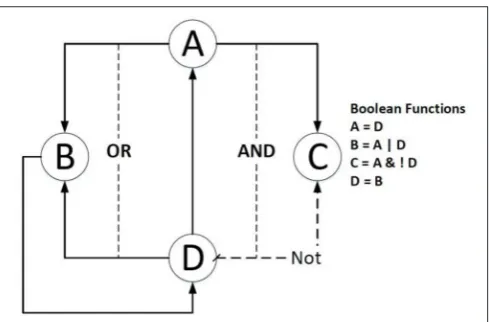
Figure 1shows an example of a Boolean network in which gene

Bis dependent on the activation of geneAor geneD, and gene

C is related to the activation of gene A and the inhibition of

geneD.

The basic premise of the Boolean network is that the genes exhibit switch-like behavior during the regulation of their functional states. The switch-like behavior ensures the movement

of a GRN from one state to another (Shmulevich et al., 2002a;

Shmulevich and Dougherty, 2005; Tušek and Kurtanjek, 2012).

FIGURE 1 |An example of a simple Boolean Network. The right side lists the Boolean functions of the example; the dashed line means the source gene is expected to be inhibited; the solid line indicates that the source gene is expected to be activated.

Boolean models can be converted into electronic circuits so that we can study the rich dynamics of Boolean networks using the signal processing theory (Xiao, 2009). Boolean models have been categorized into two main schema based on the timescales of biological events (Gershenson, 2004; Wang et al.,

2012): synchronous (also called deterministic systems) and

asynchronous schemes. In synchronous systems, all variables are assumed to have similar timescales and will be simultaneously updated, i.e., one unit will update all components simultaneously. In contrast, all variables will be updated non-simultaneously in asynchronous schemes if most of the timescales of biological events are different, i.e., each component will be updated at their own time unit (Wang et al., 2012).

Synchronous Boolean networks are based on the assumption that the state of a gene at a given time step is influenced by the state of a subset of genes in the network at the previous time step. The drawbacks of the synchronous systems are: they do not allow the temporal separation of changes in multiple regulatory events (Fauré et al., 2006), and they cannot measure differences in the speed of signal propagation as no two cells have the same properties. Hence, this results in differences in the rates of signal propagation between cells in the context of biological systems (Hwang and Lee, 2010).

The asynchronous networks only allow the update of one gene or component at a random time, resulting in a nondeterministic representation of the dynamics (Siebert, 2011). A drawback of the asynchronous scheme is that the resulting state transition graph is very complicated and encompasses many incompatible

or unrealistic pathways (Fauré et al., 2006). There are also

some modifications proposed for asynchronous Boolean models, such as non-deterministic asynchronous Boolean networks and

deterministic asynchronous Boolean networks (Gershenson,

2004).

et al. (2013) proposed an integrated hybrid model (IHM) that combines Petri nets and Boolean networks to model integrated cellular networks. The hybrid model can be applied to three main cellular biochemical processes: signal transduction, transcription regulation and metabolism (Chaouiya, 2007; Berestovsky et al., 2013).

With the facilities of the existing Boolean modeling tools, Boolean networks have been successfully applied to yeast (Kauffman et al., 2003; Li et al., 2004; Davidich and Bornholdt, 2008; Kazemzadeh et al., 2012), flower morphogenesis of wall cress: Arabidopsis thaliana (Espinosa-Soto et al., 2004),

Drosophila development (Sánchez and Thieffry, 2001; Albert

and Othmer, 2003; Ghysen and Thomas, 2003; González et al., 2008; Sánchez et al., 2008; Fauré et al., 2014), haematopoiesis (Bonzanni et al., 2013), MOMP regulation (Tokar et al., 2013),

the mammalian cell cycle or cell fate (Fauré et al., 2006;

Schlatter et al., 2009; Grieco et al., 2013; Mombach et al., 2014; Ruz et al., 2014; Cohen et al., 2015), the light- and

carbon-signaling pathways (Thum et al., 2003), apoptosis networks

(Mai and Liu, 2009; Schlatter et al., 2009; Kazemzadeh et al., 2012; Schleich and Lavrik, 2013), the hepatocyte signal networks (Schlatter et al., 2012), NF-kappaB and IL-6 mediated by miRNA (Xue et al., 2013), and leukemia (Saez-Rodriguez et al., 2007; Wittmann et al., 2009; Hwang and Lee, 2010; Saadatpour et al., 2011, 2013; Zañudo and Albert, 2013; Campbell and Albert, 2014).

In their noteworthy analysis, Davidich and Bornholdt predicted the biological cell cycle sequence of fission yeast using a Boolean model, making 47 kinetic constants that were necessary for the ODE (ordinary differential equations) approach redundant, and it was assumed that the biochemical network

was functioning in a parameter-insensitive way (Davidich and

Bornholdt, 2008). Faure et al. extended the software GINsim and studied the dynamics of a Boolean model for the control of the mammalian cell cycle, with synchronous, asynchronous

or hybrid treatment of concurrent transitions (Fauré et al.,

2006). Moreover, the signal transduction network for abscisic

acid has been proven to induce stomatal closure (Li et al.,

2006).

Currently, the most proposed biological network inference methods to identify functional modules focus either on the definition of gene regulatory networks or, more recently, on the functional networks in which an edge indicates a functional relationship and a subset of genes that describe, explain or predict a biological process or phenotype (Lazzarini et al., 2016). Far less effort has been put into the consideration of constructing activation, inhibition, and protein decay networks that could indicate the direct roles of a gene (or its synthesized protein) as an activator or an inhibitor of a target gene. The major reason for this is that the hypotheses of the current Boolean models do not provide an intuitive way to identify the individual activation or inhibition pathways of the target gene. For example, a Boolean function determines the next state of the gene expression process as eitherOn(activation) orOff (inhibition), taking into account the combined effects of the current state of its regulators (or the states of the associated regulators of the relevant gene expression processes) such as the Boolean function that describes the gene

expression status of gene CycA (Hopfensitz et al., 2013; Ruz et al., 2014), which is given by:

E2F & ! Rb & ! Cdc20 & ! (Cdh1 & UbcH10)|CycA & ! Rb &

! Cdc20 & ! (Cdh1 & UbcH10)→CycA (2)

where E2F, Rb, Cdc20, Cdh1or UbcH10 are potential genes that regulate gene CycA. As a result, a model of GRNs, including k number of genes, is constructed by the set of Boolean functions denoted asF, as given by Equation (3):

F=

fi|i=1,. . .,k , fi:{0, 1} → {0, 1} (3)

The function given by Equation (2) for CycA combines both activation and inhibition pathways that require further inferences to determine the activation and inhibition parts. The roles of the gene activator and inhibitor in this example are not intuitively defined in the compressed Boolean function even though the compressed rule can be split into multiple subfunctions. A compressed Boolean function, which is defined as a rule that contains disjunctions with various subfunctions, can be divided into a set ofAndBoolean functions by the disjunctionOr. For example, a Boolean functionP&Q|A&B&C& (D|E) can be divided as follows:

∀ = {P&Q,A&B&C&D,A&B&C&E}

where∀is a set of subfunctions. In a large GRN with many genes, this weakness becomes a significant problem in deciphering GRNs that are biologically meaningful. Furthermore, a single Boolean function determines the next status of a gene. However, this may not be true biologically because a gene may remain activated within a period of decay time when activator/activators

are not present (Albert, 2004). Also, the original Boolean

functions, as defined by Kauffman (Kauffman, 1969; Kauffman

et al., 2003), are hard-wired with the assumption of biological determinism, but genetic regulations are fundamentally

stochastic (Raj and van Oudenaarden, 2008; Xiao, 2009).

The reason for this is that the expression of a gene usually encompasses the discrete and intrinsically random biochemical reactions involved in the processes of transcription and

translation of mRNAs and proteins (Raj and van Oudenaarden,

2008). Probability Boolean networks (Shmulevich et al., 2002b; Shmulevich and Dougherty, 2005) are proposed to address the hard-wired issue by introducing stochastic components in which a gene is associated with multiple Boolean rules, and where each rule has a probability indicating the chance, and it will

impact the target gene (Raj and van Oudenaarden, 2008). The

Boolean models, in reality, may not be able to explain biological phenotypes accurately.

Therefore, to make the conventional Boolean functions clearer, we propose to focus on the general Boolean functions at the subfunction level taking into account the effectiveness of protein decay, and further split the subfunctions into the activation and inhibition domains. Because gene activation and inhibition are the two most fundamental components of complex cellular machinery, we use the term “fundamental Boolean functions” to denote these subfunctions. The biological meaning of the fundamental Boolean function is that it represents a regulatory function or regulatory complex function which can determine the activation or inhibition activity, respectively and directly. For example, Equation (2) is decomposed into six fundamental Boolean functions: CycA and E2F being TRUE trigger the activation function and Rb, Cdc20, (!E2F & !CycA) and (Cdh1 & UbcH10) being TRUE trigger the inactivation function.

In this paper, we propose a novel data-driven Boolean model, called the Fundamental Boolean Model (FBM), to draw insights into gene activation, inhibition and protein decay. This novel Boolean model provides an intuitive definition of the activation and inhibition pathways and includes mechanisms to handle protein decay as well as introducing uncertainty into Boolean functions. Furthermore, the new structure of the Boolean network allows us to propose a data mining method to extract the fundamental Boolean functions from genetic time series data. To prove the concept of the novel model, we implemented a platform using R language, called FBNNet, that is based on the proposed novel Boolean model, together with a novel data mining technique, to infer fundamental Boolean functions that visualize the dynamic trajectory of gene activation, inhibition and protein decay activities. The novel Boolean model is shown to infer GRNs with a high degree of accuracy using the time series data generated from an original cell cycle network.

The paper is prepared as follows: section Methods presents the proposed novel Boolean model and introduces a network inference method to infer networks for the model. In section Result and Discussion we present and discuss the details of the analysis results on a mammalian cell cycle network (Ruz et al.,

2014), processed with the proposed FBM. Section Conclusions

is the conclusions and discussion on the proposed FBM and experiment results.

METHODS

As discussed in the previous section, the hypotheses of the current Boolean models do not provide an intuitive way to identify the individual activation, inhibition, and protein decay of the target gene, as separate pathways. The gene activation and inhibition processes are the two primary fundamental processes of genetic regulation. Activation that increases the metabolism of drugs, for example, may result in significant drug regulatory effects, such as alterations in the metabolism ofin vivosubstances and vitamins as well as the activity of extrahepatic enzyme systems (Barry and Feely, 1990). Similarly, inhibition may result

in significant clinical drug interactions that are produced by a wide range of drugs (Barry and Feely, 1990). Inhibition is usually divided into two groups: the first group consists of reversible inhibitors that can be easily reversed by dilution or dialysis because the interactions of this group are noncovalent with

the various parts of the enzyme surface (Saboury, 2009); and

the second group contains irreversible inhibitors that usually persist even during complete protein breakdown because their

covalent bonds on the enzyme surface are strong (Saboury,

2009). Theoretically, under the assumption of an enzyme reaction exposed to the action of a reversible inhibitor, the degree of inhibition may be modeled as the reduction of the rate of reaction divided by the rate of uninhibited reaction (Saboury, 2009):

i=Vo−V

Vo

where V and Vo are the rates of inhibited and uninhibited

reactions, respectively (Saboury, 2009). The degree of inhibition (i) introduces uncertainty into the target gene. Because enzyme activation also contains the concept of the reversible type of activators, we can redefine the degree of inhibition to the degree

of enzyme reaction where V and Vo are the rates of affected

and unaffected reactions, respectively. Therefore, we can convert the equation to a conditional probability measure, which is the probability of an event that occurs given another event has happened, to represent the propensity of an enzyme reaction to reduce or raise the enzyme-catalyzed reaction rate to the target gene. If a conditional probability value of an inhibitor is 1, the inhibitor is irreversible, and if the probability is<1 and more than 0, it is reversible.

In the conventional Boolean models Equation (1) represents the processes of gene activation and inhibition which do not consider the different behaviors of enzyme reactions such as reversible and irreversible reactions. Furthermore, the disappearance of an activator does not mean the emergence of an inhibitor, i.e., a Boolean activation function with a negation sign does not mean it has to be an inhibitor. Hence, there are justifiable reasons to separate the general Boolean function into the domains of activation and inhibition. To analyse the gene activation and inhibition networks, we abstracted the characteristics of enzyme activation and inhibition, such as mutual offsetting, reversible inhibition and the long-run degradation of a specific gene product (protein). Henceforth, we propose a novel Boolean model to construct dynamic activation and inhibition networks based on this abstraction. The following section explains the proposed novel model in detail.

Definition of the Fundamental Boolean

Model

Following the same pattern as the original definition of a Boolean model, we define our novel Boolean network as a graph G (X, Ea,Ed), where the node collection, V = {v1,v2,. . .,vn}

corresponded to a group of states, X = {xi|i = 1,. . .,n}

of size n, where each variable is only in one of two states:

On (1) or Off (0), and the general edge set, E, was divided

which are categorized by their regulatory functionalities, i.e., the activation and inhibition, rather than a single function, as in all conventional Boolean models. We denote this graph as a Fundamental Boolean Network (FBN) and the two sets of fundamental Boolean functions are defined as

-Fundamental Boolean functions of activation:

F_ai = n

f_ai_j|j=1,. . .,la(i)

o

, f_ai_j:{0, 1} → {−, 1} (4.a)

Fundamental Boolean functions of inhibition:

Fi_d= n

f_di

k|k=1,. . .,ld(i) o

, f_di

k:{0, 1} → {−, 0} (4.b)

whereF_aiandF_di present a set of fundamental Boolean activiation and inhibition functions for the target genei, respectively. “–” means the output of the function has no impact on the target gene. la(i) denotes the total number of fundamental Boolean

functions activating the target gene and l_d(i)denotes the total number of fundamental Boolean functions deactivating the target gene. The output of a fundamental Boolean activation function

is TRUE means the target gene will be activated and FALSE

means the activation function has no impact on the target gene. Similarly, The output of a fundamental Boolean inhibition

function is TRUE means the target gene will be inhibited and

FALSEmeans the inhibition function has no impact on the target gene.

The proposed fundamental Boolean functions encapsulate the following biologically meaningful key ideas:

• A fundamental Boolean function is a simple transition rule that takes a minimum group of essential gene states as an input and determines the regulation effect on the target gene in the form of a Boolean value.

• In general, a fundamental Boolean function is a function that cannot be divided any further. Hence, a fundamental Boolean function can be regarded as a delegation of stereochemical reactions, such as the activity of a transcription factor formed by the binding of a few essential proteins; a combination of transcription factors formed containing multiple transcription factors; a transcription factor complex formed by binding a transcription factor with other proteins; and, conditions that constrain gene activity.

• A general assumption of the proposed fundamental Boolean functions is that the production of the coded protein for each gene at each time step is either completely activated or inhibited. A further assumption is that gene regulation can be entirely or partially affected by the recipe defined by a fundamental Boolean function that states how proteins bind to their target genes.

• The gene regulation time is embedded into Boolean updating schema based on the treatment of time. Under the synchronous scheme, all states have a unique successor, i.e., all nodes are updated at the same time, and all gene regulation processes are assumed to have completed upon the next time step. This scheme is simple but induces well-known artifacts (Fauré et al., 2006). With the asynchronous scheme, the result may be closer to biological reality but could be

more computationally challenging to evaluate because every transition is updated at a different time step.

The output of the proposed functions reflects only the potential effectiveness of gene regulation on the target gene. Therefore, we need to make sure how confident we are to trust the regulatory functions that can impact on the target gene. As discussed previously, the degree of enzyme reaction can be replaced by the conditional probability of the event that an enzyme reaction can affect the target gene. Hence, the concept of conditional probability is then applied to measure the general confidence of the proposed functions. The following formulae, denoted as confidence measures, calculated the conditional probability of each fundamental Boolean function separated by the activation and inhibition of genes.

Confidence measure of activation:

C_ai_jjf_ai_jAj_i(t) k

= pσ_it+1=1|Aj_i(t)=1

=

pAj_i(t)=1∩ σ_it+1=1

pAj_i(t)=1 (5.a)

Confidence measure of inhibition:

Ci_d

k j

f_di

k

Dk_i(t) k

= pσ_it+1=0|Dk_i(t)=1

=

pDk

i(t)=1∩ σit+1=0

pDk_i (t)=1

(5.b)

Whereσ_it represents the Boolean state of geneiat time t, and σ_it+1 represents the Boolean state of geneiat time t+1. ∩ is a logical And connector. Ci_aj and Ci_d

kdelegate the confidence function with the input of the fundamental Boolean functions

fi aj andf

i

dk, respectively.A j

iandDki represent the set of required

inputs for the gene state functions, f_ai_j and f_di

k, respectively.

Aj_i(t) = 1 or Dk_i(t) = 1 mean the required gene input of f_ai_j or f_di

classic example of the lac operon discussed in (Edwards and Bestor, 2007).

There are debates on the decay time of mRNA/proteins

in Boolean models that allow the gene to remain in the On

state when no activators or inhibitors are present. Réka Albert proposed that this decay may happen in two time steps because the decay time of a protein in an inactive state is usually longer than the time taken for its synthesis (Albert, 2004). To encapsulate the factor of protein decay, we denote a function

fdecay (given below) to summarize the requirements of protein

degradation with input from the target geneiat timet:

f_decay σ_it,ϑ

= ¬(τ ≤ϑ )×σ_it (6)

where τ represents an incremental variable presenting the

number of time steps that have been processed. The τ will be

reset to 0 whenever there is any fundamental Boolean function having an effect on the target geneiat timet +1.ϑ delegates the decay time period to reflect the fact that the attenuation

or enhancement of the expression of mRNA requires time. ¬

represents a negation operator that changes a Boolean function fromTRUEtoFALSEor vice versa.×is a logicalAndoperator.

The output of the decay function f_decay is a Boolean value of

On(1) at time t +1 if the gene state ofσi at timet isOn(1)

within the tolerated time period orOff(0) at timet+1 when the tolerated time period is expired regardless of the gene state ofσ_i at timet. We assume that the tolerated time period for protein decay has only one time step for short time series data. Short time series data contain an enormous number of genes but only a few observations; hence, knowledge of the mechanistic details and kinetic parameters cannot be extracted consistently from the data (Ernst et al., 2005; Wang et al., 2008; Chaiboonchoe, 2010). About 80% of published experimental data are short time series because the expenses involved in acquiring genetic data are not economic and the time taken to examine the patients is usually too short due to health issues (Ernst et al., 2005; Wang et al., 2008; Chaiboonchoe, 2010). With regard to long time series data, which contain more observations than short time series data, we assume the tolerated time period is in two time steps to match the decay assumptions of Réka Albert (Albert, 2004).

By combining Equations (4.a, 4.b), (5.a, 5.b), and (6) we propose the novel Boolean model (FBM) as:

σ_it+1 = f_decay(σ_it,ϑ)+ ∨la(i) j=1

n

P

Ci_aj

f_ai_j(Aj_i(t))o

׬ ∨ld(i) k=1

n

P

Ci_d

k

f_di

k(D k i(t))

o

(7)

The role offdecay(σit,ϑ) in Equation (6) is to ensure that if no

activators are present, the gene state σ_i at time t +1 depends on the state of itself at timetif it is tolerated by the parameter ϑ, a decay time period.P

x

is a Boolean function that takes a

uniform distributed random number,µ, and an output of 1 ifµ

<x and 0 otherwise. V{x} denotes the logical connective function ofOr, i.e.,Vla(i)

j=1{Fai}=fai1+f i

a2+. . .+f i

a_la(i)if all activation rules

of geneihave the confidence measure value of 1.+is a logical

Oroperator. The output of the proposed model is the activation or inhibition status of the target geneiat timet +1. A general

assumption of the proposed model is that all gene regulations are controlled by the proposed fundamental Boolean functions in the activation, inhibition and protein decay domains.

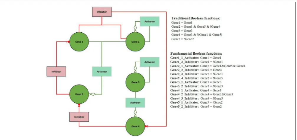
Figure 2illustrates an example of FBN. The terms activator and activation function, and inhibitor and inhibition function are interchangeable throughout this paper. The left hand side presents a wiring diagram of FBNs; the top right hand side is a list of Boolean functions in the form of traditional Boolean models; the bottom right hand side has a list of fundamental Boolean functions. Both sets of functions have identical functionalities but the second set displays the rules separated by the types of

activators and inhibitors (seeSupplementary Information for

an example of the calculation of fundamental Boolean function). The proposed model can simulate the dynamic equilibrium

of gene regulation. Figure 3illustrates an example of how the

proposed model (FBM) can handle the dynamic equilibrium of gene regulation. In this example, gene A is an activator for gene B, but gene B is an inhibitor of gene A. The result is an equilibrium of both A and B. The FBM parameters are: the time step for protein decay is 1; the time step for a gene to complete its regulation process is 1; the confidence measure for each rule is 1 (100%). The Boolean updating schema is the synchronous scheme. In case 1, Gene B was activated by Gene

A at the time step 2. Gene A was turnedOff due to the protein

decay at the time step 2. Gene B was turned Off at the time

step 3, which is also due to the protein decay. In case 2, Gene A was inhibited by Gene B at the time step 2, and Gene B was continually boosted up by Gene A at the time step 2 but inhibited due to the protein decay at the time step 3. In case 3, Gene A was inhibited by Gene B and Gene B was turned

Off due to the protein decay at the time step 2. In case 4, both genes were entrapped into a simple loop, namely, attractor due to the lack of activators to turn any of themOn. All of the cases will be entrapped into the same attractor, i.e., the gene state of {0,0}.

FIGURE 2 |Example of a Fundamental Boolean Network. The icon box is denoted as a fundamental Boolean function. The red box is denoted as an inhibition function, and the light green box is denoted as an activation function. The green circle icon is denoted as a gene or a variable.

FIGURE 3 |Simulation of the dynamic equilibrium of gene regulation.

methodology to extract the fundamental Boolean model related networks.

Inference Network With an Analytical Cube

There are two main steps to inferring fundamental Boolean networks from time series data. The initial phase is to construct a

cube type database to store all important precomputed measures. The precomputed measures are listed as follows (see SI for the example of each measure):

• Confidence Measures:

a conditional probability on the causality of regulation between a conditional gene, at timet, and the target gene, at timet+1.

• Confidence Counter Measures:

Confidence counter measures are similar to the confidence measures introduced in Equations (5.a) and (5.b) but are used to indicate the conditional probability on the causality of the target gene, at timet, which regulates the conditional gene

at timet + 1. We denote the confidence counter measures

asC∀i_aj and C∀i_d

k for activation and inhibition, respectively, then we applied the following formula to calculate the value of the confidence counter. The outputs,C∀i_aj and C∀i_d

k are conditional probabilities and, hence, the range of the value is between 0 and 1.

Confidence counter measures of activation:

C∀i_aj j

f_ai_jAj_i(t+1) k

= pAj_i(t+1)=1|σ_it=1

=

pAj_i(t+1)=1∩ σ_it =1

p σ_it=1 (8.a)

Confidence counter measures of inhibition:

C∀i_d k

j

f_di

k

Dk_i(t+1) k

= pDk_i(t+1)=1|σ_it=0

=

pDk_i(t+1)=1∩σ_it =0

p σ_it =0 (8.b)

• Support Measures:

Support measures are the percentage of transactions contain marched rules (Aj_i(t) = 1∩σ_it+1 = 1 andDk_i(t) = 1∩σ_it+1=0) over all time steps in all samples. Let us denote the total number of time steps involved asℵ

ℵ =

s

X

i=1 (ti−1)

whereti is the number of time steps of sample i and s is

the total number of samples. The first time step of samplei

is not included because the calculation of support measure

involves two time steps (t and t + 1). We denote the

support measures asSi aj andS

i

dkfor activation and inhibition respectively. Therefore, the activation and inhibition of the support measurements for geneiare definded as:

Support measure of activation:

Si_aj =

countAj_i(t)=1∩σ_it+1=1

ℵ (9.a)

Support measure of inhibition:

Si_d

k=

countDk_i (t)=1∩ σ_it+1=0

ℵ (9.b)

• Conditional Causality Test:

Some researchers claimed that causality is not a concept statistic and is not statistically ‘identifiable’ because a secluded causal hypothesis cannot be verified by using only observational data (Simcha et al., 2013). However, we believe that the direction between the conditional gene and the target gene is still able to be calculated based on the conditional probabilities between the conditional gene and the target gene using the following formulae:

Conditional causality test= Confidence measure

Confidence counter measure

(10) The formulae for calculating the confidence measures and the confidence counter measures have been discussed in Equations (5.a, 5.b) and (8.a, 8.b). The ratios and interpretations are based on plausibility reasoning theory: if geneBat timetcauses geneA, at timet+1, to be expressed, then the confidence ofp(At+1 = 1|Bt = 1) is equal to 1; in

contrast, the reasoning that geneBat timet+1 is caused by geneAat timetmay not be as strong as geneAat timet+1 caused by geneBat timetdue to lack of information to support this reasoning. Hence, confidence p(Bt+1 = 1|At = 1) is

≤p(At+1 =1|Bt =1). The ratiop(At+1=1|Bt =1) divided

byp(Bt+1 = 1|At = 1), can then be used as a test for the

causality direction between genesAandB. We named this test a conditional causality test. This test can differentiate indirect regulators from direct ones because the indirect regulators will usually have weaker reasoning than the direct ones.

Therefore, by giving confidence for a potential fundamental Boolean function and a confidence counter for the potential fundamental Boolean function, we can calculate the value of the conditional causality test and interpret it as follows:

• If the value of the conditional causality test for target gene

Aand the conditional geneBis greater than 1, geneA, then, is regulated by geneB.

• If the value is equal to 1, genesAandBare then regulated from each other.

• If the value is lower than 1, there is no causal relationship, so the hypothesis that geneBregulates geneAcan be rejected.

• Entropy and Mutual Information:

The Shannon entropy theory provides a quantitative information measure about the probability of observing a particular symbol, or event,Pi, within a given sequence

H= −XPilogPi

where log is a logarithm with base 2. The sequence is the

sum of the probabilities of an event being eitherOnorOff

(Shannon, 1948; Shannon and Weaver, 1963; Liang et al., 1998). Moreover, mutual information is defined as:

M(X,Y)=H(Y)−H(Y|X)=H(X)−H(X|Y)

FIGURE 4 |Illustration of an orchard cube.

Y (Liang et al., 1998). M(X,Y) presents the remaining information between sequence X and the information shared between X and Y. The output state of X is determined by Y if

M(X,Y) =H(X) (Liang et al., 1998). Hence, we can use this measure to find the causality relationship between genes.

The mutual information and Shannon entropy measures are assumption-free methods measuring unknown and complex associations; however, they have the limitation of overestimating the regulation relationships leading to possible failures, such as the inability to differentiate indirect regulators from direct

ones, as cited by Liu et al. (Liu et al., 2016). To overcome

this limitation, we combined the mutual information measures with the conditional causality test we proposed as an important mechanism to extract the regulatory rules. As mentioned previously, the conditional causality test can differentiate indirect regulators from direct ones and is complementary to the mutual information measures.

Orchard Cube

A data cube is used to store precomputed measures for data mining. Many familiar genetic time series data are multidimensional, containing genes, time steps, and samples. Analysing multidimensional data could run into performance bottlenecks but precomputing a data cube can release performance bottlenecks by providing scalable mechanisms for fast access to the summarized data (Han et al., 2012). To

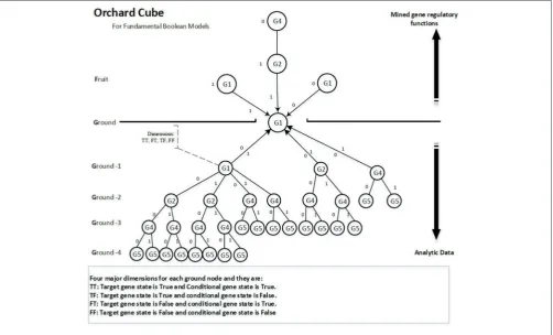
infer the activators and inhibitors, we extend the data mining technique of bottom-up computation (BUC), which is an algorithm for the computation of sparse cubes from the Apex cuboid downward (Han et al., 2012) to a prefix tree type of cube, as shown inFigure 4. We call this cube the orchard cube because it looks like an orchard containing many fruit trees.

Each branch or link above ground on the tree is a regulatory function. Every node on a branch is a component of the regulatory function. Because regulatory functions are the

knowledge we are looking for, we call them fruit. The gene

nodes on the ground are called seeds. The training data are

called fertilizers as they help the trees to grow larger (more

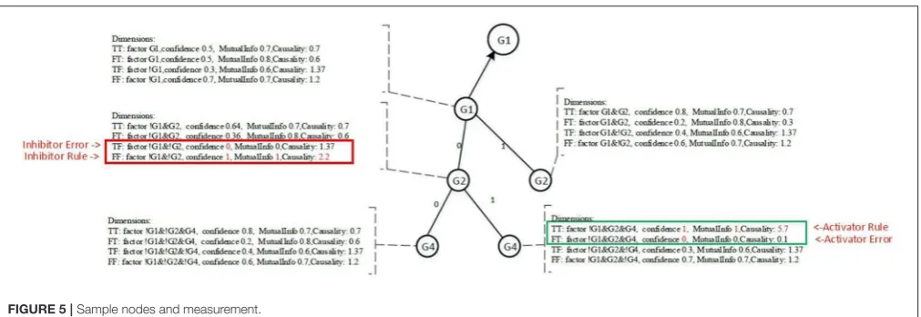
FIGURE 5 |Sample nodes and measurement.

The nodes underground are analytical data that contain all possible regulatory functions for the target gene unless the NULL hypothesis rejects them. The nodes above ground comprise the extracted regulatory functions that have been mined from the nodes underground. Hence, if we define the collection of regulatory functions of a target gene as U`` and the analytic data part as

˘

U, then U``∈

˘

U.

Pairwise Dimensions

Each node contains four dimensions, i.e., four major groups of measures. Each dimension represents a potential regulatory function of the target gene. The four dimensions are denoted as TT, TF, FT, and FF, as shown inFigure 5, and are defined as follows:

• TT is when the target gene’s state is TRUE, the current conditional gene state is TRUE, and all upstream conditional gene states are fixed;

• TF is when the target gene’s state is TRUE, the current conditional gene state is FALSE, and all upstream conditional gene states are fixed;

• FT is when the target gene’s state is FALSE, the current conditional gene state is TRUE, and all upstream conditional gene states are fixed;

• FF is when the target gene’s state is FALSE, the current conditional gene state is FALSE, and all upstream conditional gene states are fixed;

All nodes under Ground-2 will have prefix gene states.

For example, conditional gene, G4, of target gene G1 at

Ground-3 has its two upstream gene states fixed, i.e., G1(0)

and G2(0), therefore, the four dimensions of the node

G4 are TT (G1|!G1&!G2&G4), TF (G1|!G1&!G2&!G4), FT (!G1|!G1&!G2&G4) and FF (!G1|!G1&!G2&!G4). Each dimension has a factor, also called a function statement, which represents the potential gene regulatory function. Dimensions TT and FT, FT and FF are two pairwise dimensions. The minimum confidence measures between TT and FT, FT and FF are error measures. The pairwise dimensions have the following characteristics:

P(TT)=1−P(FT)and P(TF)=1−P(FF)

For the pair dimensions, if we define one dimension to be the confidence measure that will have an impact on the target gene, the other dimension is then regarded as an error measure. This definition is equivalent to the definition of the essential Boolean statexithat must match the requirements of

f x1,. . .xi−1, 0,xi+1,. . .,xn 6= f x1,. . .xi−1, 1,xi+1,. . .,xn

for allx1,. . .xi−1,xi,xi+1,. . .,xn, wheref is a Boolean function

andxiis a Boolean state (Fauré et al., 2006). The output off is a

Boolean value.

Orchard Cube Pruning

Constructing the cube requires building an optimal tree-type data structure from all possible combinations of all related genes up to a maximum depth. The computational cost grows exponentially. However, it is endurable because all precomputed genes will not go to next level to avoid redundant computations. For example, we have three genes,A, B, C, and the conditional probability of geneAand gene Bregulating the expression ofC isp(C|A,

B). Because p(C|A, B) is equal to p(C|B, A), the branch for precomputing p(C|B, A) is not processed from the main tree. Hence, the computational cost of constructing the entire cube is affordable.

Before the initial pruning, we use Pearson’s Chi-square test (Plackett, 1983) to test the NULL hypothesis that a target gene is independent of the gene selected as the conditional gene. All genes in GRNs apart from the target gene will be tested using this criterion to remove unrelated genes from Ground-2 when thep-value is over 0.05. This procedure reduces unnecessary root branches.

cost of processing each target gene can be reduced dramatically; however, this process is uneven.

The Algorithm to Construct the Orchard Cube

To build the orchard cube, we use the step-by-step algorithm below:

1. All genes are potential target genes; hence, we put all the genes asseedson the ground level and partition them intoN

trees.Nis the total number of genes. Because the construction of all trees is partitioned and parallel we explain the further steps for one tree only. The result is an orchard cube type of data structure that contains all precomputed measures, as discussed previously.

2. With target genei, we first use the Chi-square test to test the NULL hypothesis of the target gene, against all other genes, for no relationship between them, as discussed previously. 3. We look through all potential regulatory genes and calculate

all measures for the four dimensions, i.e., the TT, TF, FT, and FF, as discussed previously.

4. If the current underground level is lower than a value named

maxK denoting the maximum underground level the tree

can penetrate into, all potential regulatory genes, exclude the current gene and the genes that are already in the higher levels, will go to the next level.

5. In the next level, we repeat steps 3 and 4 until the current level is equal tomaxKor all related genes are processed.

6. If the current level is equal to maxK or all relevant genes

are processed, the construction of the current tree is then completed.

7. If all target genes have been processed, we then output the cube.

Inferences of Fundamental Boolean Networks

The second phase is to mine fundamental Boolean functions

from a cube type database structure. Figure 6 presents a

schematic diagram of fundamental Boolean network inference. As outlined inFigure 6, to infer FBNs we need to extract all essential measures, as explained previously, from a set of training data. The precomputed measures are then stored in a cube type database structure so the end users can generate different strategies to mine fundamental Boolean functions from the cube. The mined FBNs are then used to reconstruct time series to either trace the Boolean attractors or to verify the network generated by comparing the reconstructed time series data with the original training data.

Using the proposed orchard cube, we can infer interactions between the genes in the GRNs by filtering each tree’s underground part based on the criteria listed below:

1. The conditional causality test value should be>1 or equal to 1. 2. The mutual information test should be equal to 1 or between

a threshold and 1 when the time series data contain noise. 3. Discard the functions if they are matched with the following

patterns because they are not essential states.

f_ai_j(A&B&C) = f_ai_j(A&B&!C) or

f_di

j(A&B&C) = f i

dj(A&B&!C)

4. The confidence measure value should be greater than a threshold, e.g., 0.7, to include some functions that contain noise. However, this criterion should be varied according to the noise level of the data.

5. Sort all functions remaining after step 4 by the mutual information measure, error measure, support measure and the number of genes input. Ideally, we want to keep the rules that have a more substantial support value with minimum errors. 6. The total number of fundamental Boolean functions for each

type (activation or inhibition) of a gene is a limited to Fn based on different experimental requirements. However, in this study, we take Fnto be 5.

Reconstruction of Time Steps

The model, formulae and orchard cube we introduced in the previous section provide a complete mechanism to calculate the next gene state at timet+1 by giving the gene state at timet. Therefore, we can reconstruct the time steps to any length by giving the initial gene state at timet=0. The following list gives the primary usages of applying the model to reconstruct time steps:

Verify the reconstructed time series data against the original time series. The regulatory functions are a subset of the analytic data. If the functions are correct, we should be able to reconstruct time steps with the same initial states as the original time series. Because the asynchronous Boolean model produces an undetermined result, the reconstructed time series data might be different from the training time series data. Hence, we focus on demonstrating the FBM using synchronous Boolean schema only in this paper.

Reconstruct the hidden layers between the observed time steps. In short time series data, the gaps between observed time steps are very sparse. We can use the reconstructed time series to reveal the hidden layers by giving the initial Boolean state and keeping on generating the next time step based on the previous time step until the latest generated time step is identical to the next observed time step. By giving the two observed states

Sobserved1 andSobserved2, we reconstructed the time series data, as

follows:

Sreconstructed=S1,S2. . .Sk, Sobserved1=S1 and Sobserved2=Sk

The states betweenS1andSkare then denoted as missing time

steps or hidden layers.

RESULT AND DISCUSSION

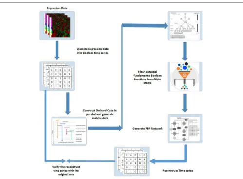
FIGURE 6 |Schematic diagram of FBN modeling and network inferences: (1) discrete expression data into Boolean time series; (2) construct orchard cubes in parallel to generate analytical data and store all precomputed measures; (3) mine potential regulatory rules for all target genes through the constructed orchard cube based on some criteria; (4) generate the fundamental Boolean network; (5) use the generated network to reconstruct the input time series by giving the initial states of all original inputs and; (6) verify the reconstruction time series with the original series, if necessary, to gain confidence in the results.

subfunction is extracted using the methodology we proposed. To extract the fundamental Boolean network, we implemented

an R package, namelyFBNNet(Fundamental Boolean Network

toolset, a prototype version is available at https://github.com/ clsdavid/FBNNet_Lincoln), which can build an Orchard type of

cube and mine FBNs from the cube. TheFBNNettool can find

attractors under the two main Boolean updating schema and plot a static regulatory graph as well as a dynamic regulatory graph. The following paragraphs describe the main experiment we conducted.

Experimental Design and Dataset

The experiments conducted and described here intend to prove

the concept of the new Boolean Model, i.e., the FBM.Figure 7

outlines the experiment design as a benchmark to compare

the results generated via BoolNet (Müssel et al., 2010) with

those consequently reconstructed from the new R package,

FBNNet. TheBoolNetpackage was demonstrated in the tutorial

of (Hopfensitz et al., 2013) and the study ofRuz et al. (2014). The advantage of theBoolNetpackage over other existing tools, such as GINsim (Gonzalez et al., 2006), BooleanNet (Albert et al.,

2008) and BN/PBN toolbox in Matlab, is the support of all

three network types.FBNNetis a new R package that we have

implemented for testing the concept of the FBM, and it has been fully integrated with the algorithms and concepts we introduced in section Methods.

FIGURE 7 |Experiment design of evaluating the Fundamental Boolean network inference. The blue arrows represent the processes using BoolNet and brown arrows represent the processes using our FBNNet tools. The green arrows represent the evaluation process.(A)We use the BoolNet script loadNetwork.R to load pre-defined networks from files and then generate the time series and networks.(B)We use the time series generated from BoolNet and the new R package, FBNNet, to generate FBNs.(C)We reconstruct the time series via the FBM.(D)To evaluate the FBM, we rebuild the BoolNet type network based on the reconstructed time series; and(E)we evaluate the FBN inference methods by comparing the generated time series and the generated BoolNet type of network with the original time series and network that were generated in step A.

itself contains four different sub-phases (prophase, metaphase, anaphase, and telophase) (Fauré et al., 2006). The S and M phases involve two gap phases, namely G1 and G2 (Fauré et al., 2006).

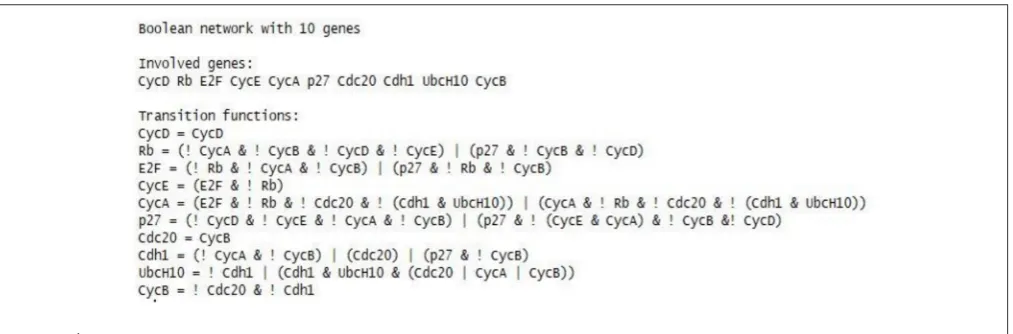
To generate the experimental data, firstly, we used the

command loadNetwork from BoolNet to load the cell cycle

network specified in the text files: cellcycle.txt, as shown in Figure 8. Secondly, we use the method generateTimeSeries of

BoolNet to generate 1024 noiseless sample data with 43 time steps for the cell cycle network, with all default settings, i.e., the parametertypeis synchronous, the parameternoiseLevelis 0, and the parameter perturbations is 0. Each sample contains the same 10 mammalian cell cycle genes, i.e., CycD, Rb, E2F, CycE, CycA, p27, Cdc20, Cdh1, UbcH10, and CycB, as the study conducted by Hopfensitz et al.(2013). The generated 1024 sample data are the dataset used for this experiment. Each sample contains 43 time steps in sequence. All the initial states of the 1024 samples are unique containing the complete combination of 210_changes. Hence, the number of genes that are expressed in each sample is variant.

Because the proposed Boolean rule definition is very different from the traditional Boolean rules, i.e., intuitive rules vs compressed rules (not intuitive) as discussed in section Background, we cannot compare it with other networks generated by other tools directly as it would not be a fair

comparison. Hence, the best way to evaluate the generated FBNs is to use them to reconstruct time series data with the same initial states and then compare with the training time series data. The reason is that under the synchronous model if the generated network is correct, the network should be able to produce the same time series data as the training time series data with the same initial states.

The evaluation matrix for the time series comparison we have adopted is ER (Error rate), AR (Accurate rate), MMR (Mismatched rate) and PMR (Perfect matched rate). The matrix is defined as follows:

ER = Pn

i=1num of unmatched state per sample(i)

n

AR = Pn

i=1num of matched state per sample(i)

n =1−ER

PMR = Num of 100% matched sample matrixes

n

MMR = Num of unmatched sample matrixes

n =1−PMR

FIGURE 8 |Known mammalian cell cycle networks provided byBoolNet.

contains gene states (Boolean value). Hence, a sample data means a sample matrix in this paper.

FBN of Cell Cycle and Its Validation

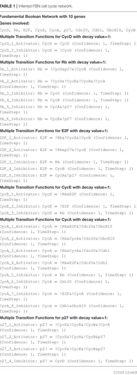
The FBN for the sample genes and the FBN for the cell cycle genes were inferred via the R packageFBNNet, as shown inTable 1.

As shown in Table 1, three primary parameters are bound

with this novel FBN, and they are confidence (Equation 5), protein decay (Equation 6) and time step. The two parameters, time step and protein decay, were configured to 1 to match the way of generating the experimental data via the method

generateTimeSeries ofBoolNet. The method generateTimeSeries

ofBoolNetdoes not provide a configurable parameter for protein decay but has a default value of 1 (time step), embedded inside its logic.

A significant difference from other existing Boolean models is that the inferred FBN splits the Boolean functions of the mammalian cell cycle into the domain of activation and

inhibition intuitively as shown inTable 1. Each gene could be

regulated by multiple activation rules or inhibition rules at the same time. The result inTable 1shows that the uncertainty of the process can be incorporated into the model. All FBM functions have the parameter confidence of 1, means the result is extremely accurate. To verify the result, we used the initial states from the training time series dataset to regenerate the same size data set using the novel concept of FBM (Equation 7) under the synchronous updating schema (same as the schema when the training dataset is generated). The regenerated dataset, then, is compared with the training time series dataset.

As shown inTable 2, all reconstructed time series data from the mammalian cell cycle network are identical to the pre-generated time series data with 100% in both AR and PMR. 100% of AR and PMR means all regenerated time series data are matched with the training time series dataset. Hence, we believe the inferred FBN cell cycle network with the proposed FBM is an alternative way to represent the mammalian cell cycle network but provides more information to draw insights into the activation and inhibition pathway of the mammalian cell cycle network.

Regarding FBNs, Figure 9 present the regulatory graph of

the cell cycle network. The graph is generated by integrating the mined FBNs with the R package visNetwork (see online documentation http://datastorm-open.github.io/visNetwork/).

As shown in Figure 9, the internal relationships between

genes are displayed. Hence, we can explore how these genes activated and inhibited other genes by tracing the input genes and the target genes via activators and inhibitors. The FBN of cell cycle contains three type of connections in the domains of gene activation, gene inhibition and protein decay.

Attractors

Attractors are defined as recurrent cycles of states (Hopfensitz et al., 2013), which are of particular interest in Boolean modeling. When a network reaches an attractor, it entraps a cycle most of the time until external perturbations happen to alter some essential genes’ production to let the network get out of the entrapment. With the simplest synchronous assumption, we yield 2 attractors as shown inFigure 10. One is a stable attractor, and the other is cycle attractor. The attractors are equivalent to the findings that have been reported in (Fauré et al., 2006; Hopfensitz et al., 2013). Hence, the FBN of the cell cycle can produce the same attractors as other Boolean models did.

The first attractor is a simple attractor with only Rb, p27 and Cdh1 active, and is associated with the phase G0 or cell quiescence (Fauré et al., 2006). The CycD represents the whole cdk4/6-Cyclin D complex, and cdk4/6 is a cyclin-dependent kinase (cdk) partners.

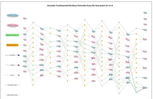
The richness of the proposed model was its dynamic networks that provided a complete trajectory of gene activation, inhibition

and protein decay.Figure 11presents the dynamic trajectories

TABLE 1 |Inferred FBN cell cycle network.

Fundamental Boolean Network with 10 genes

Genes involved:

CycD, Rb, E2F, CycE, CycA, p27, Cdc20, Cdh1, UbcH10, CycB

Multiple Transition Functions for CycD with decay value₌1:

CycD_1_Activator: CycD = CycD (Confidence: 1, TimeStep: 1)

CycD_2_Inhibitor: CycD = !CycD (Confidence: 1,

TimeStep: 1)

Multiple Transition Functions for Rb with decay value₌1:

Rb_1_Activator: Rb = !CycD&p27&!CycB (Confidence: 1,

TimeStep: 1)

Rb_2_Activator: Rb = !CycD&!CycE&!CycB&!CycA

(Confidence: 1, TimeStep: 1)

Rb_3_Inhibitor: Rb = CycD (Confidence: 1, TimeStep: 1)

Rb_4_Inhibitor: Rb = CycB (Confidence: 1, TimeStep: 1)

Rb_5_Inhibitor: Rb = CycA&!p27 (Confidence: 1,

TimeStep: 1)

Rb_6_Inhibitor: Rb = CycE&!p27 (Confidence: 1,

TimeStep: 1)

Multiple Transition Functions for E2F with decay value₌1:

E2F_1_Activator: E2F = !Rb&!CycA&!CycB (Confidence: 1,

TimeStep: 1)

E2F_2_Activator: E2F = !Rb&p27&!CycB (Confidence: 1,

TimeStep: 1)

E2F_3_Inhibitor: E2F = Rb (Confidence: 1, TimeStep: 1)

E2F_4_Inhibitor: E2F = CycB (Confidence: 1, TimeStep: 1)

E2F_5_Inhibitor: E2F = CycA&!p27 (Confidence: 1,

TimeStep: 1)

Multiple Transition Functions for CycE with decay value=1:

CycE_1_Activator: CycE = !Rb&E2F (Confidence: 1,

TimeStep: 1)

CycE_2_Inhibitor: CycE = !E2F (Confidence: 1, TimeStep: 1)

CycE_3_Inhibitor: CycE = Rb (Confidence: 1, TimeStep: 1)

Multiple Transition Functions for CycA with decay value=1:

CycA_1_Activator: CycA = !Rb&E2F&!Cdc20&!UbcH10

(Confidence: 1, TimeStep: 1)

CycA_2_Activator: CycA = !Rb&CycA&!Cdc20&!UbcH10

(Confidence: 1, TimeStep: 1)

CycA_3_Activator: CycA = !Rb&CycA&!Cdc20&!Cdh1

(Confidence: 1, TimeStep: 1)

CycA_4_Activator: CycA = !Rb&E2F&!Cdc20&!Cdh1

(Confidence: 1, TimeStep: 1)

CycA_5_Inhibitor: CycA = Rb (Confidence: 1, TimeStep: 1)

CycA_6_Inhibitor: CycA = Cdc20 (Confidence: 1,

TimeStep: 1)

CycA_7_Inhibitor: CycA = !E2F&!CycA (Confidence: 1,

TimeStep: 1)

CycA_8_Inhibitor: CycA = Cdh1&UbcH10 (Confidence: 1,

TimeStep: 1)

Multiple Transition Functions for p27 with decay value=1:

p27_1_Activator: p27 = !CycD&!CycE&!CycB&!CycA

(Confidence: 1, TimeStep: 1)

p27_2_Activator: p27 = !CycD&!CycA&!CycB&p27

(Confidence: 1, TimeStep: 1)

p27_3_Activator: p27 = !CycD&!CycE&!CycB&p27

(Confidence: 1, TimeStep: 1)

p27_4_Inhibitor: p27 = CycD (Confidence: 1, TimeStep: 1)

(Continued)

TABLE 1 |Continued

p27_5_Inhibitor: p27= CycB (Confidence: 1, TimeStep: 1)

p27_6_Inhibitor: p27= CycA&!p27 (Confidence: 1,

TimeStep: 1)

p27_7_Inhibitor: p27= CycE&!p27 (Confidence: 1,

TimeStep: 1)

p27_8_Inhibitor: p27= CycE&CycA (Confidence: 1,

TimeStep: 1)

Multiple Transition Functions for Cdc20 with decay value=1:

Cdc20_1_Activator: Cdc20 = CycB (Confidence: 1,

TimeStep: 1)

Cdc20_2_Inhibitor: Cdc20 = !CycB (Confidence: 1,

TimeStep: 1)

Multiple Transition Functions for Cdh1 with decay value=1:

Cdh1_1_Activator: Cdh1 = Cdc20 (Confidence: 1,

TimeStep: 1)

Cdh1_2_Activator: Cdh1 = !CycA&!CycB (Confidence: 1,

TimeStep: 1)

Cdh1_3_Activator: Cdh1 = p27&!CycB (Confidence: 1,

TimeStep: 1)

Cdh1_4_Inhibitor: Cdh1 = !Cdc20&CycB (Confidence: 1,

TimeStep: 1)

Multiple Transition Functions for UbcH10 with decay value=1:

UbcH10_1_Activator: UbcH10 = !Cdh1 (Confidence: 1,

TimeStep: 1)

UbcH10_2_Activator: UbcH10 = Cdc20&UbcH10 (Confidence: 1,

TimeStep: 1)

UbcH10_3_Activator: UbcH10 = UbcH10&CycB (Confidence: 1,

TimeStep: 1)

UbcH10_4_Activator: UbcH10 = CycA&UbcH10 (Confidence: 1,

TimeStep: 1)

UbcH10_5_Inhibitor: UbcH10 = Cdh1&!UbcH10 (Confidence: 1,

TimeStep: 1)

Multiple Transition Functions for CycB with decay value=1:

CycB_1_Activator: CycB = !Cdc20&!Cdh1 (Confidence: 1,

TimeStep: 1)

CycB_2_Inhibitor: CycB = Cdh1 (Confidence: 1, TimeStep: 1)

CycB_3_Inhibitor: CycB = Cdc20 (Confidence: 1,

TimeStep: 1)

TABLE 2 |Experimental results for reconstructed time series data.

Network Number

of samples

Number of time

steps

ER AR PMR MMR

Cell cycle 1,024 43 0 100% 100% 0

displayed. For example, inFigure 11, the CycD deactivates Rb

FIGURE 9 |Cell Cycle FBN. The light blue elliptical icons represent genes; the orange box icons represent inhibition functions, and the light green box icons represent activation functions. The dark blue arrows represent activation, dark red arrows represent inhibition, and gray arrows represent protein decay.

phosphorylates E2F, CycA, and CycE, and the promotion of p27 enhances Cdh1. Rb continues to be activated without the interruption of CycB, CycA, CycE, and CycD. The UbcH10 at the time step of 3 is inhibited as the consequence of protein decay (see the gray dash arrow line) because none of its activation and inhibition functions has an impact on it.

As shown through the demonstration of the proposed model with the mammalian cell cycle, we demonstrate that we could use the proposed orchard cube to infer the GRNs of the mammalian cell cycle. The outcome shows that if the network inferred was 100% correct, the reconstructed time series should match 100% with the original training dataset. However, this assumption was based on the degree of completeness of the initial training dataset when used with the synchronous Boolean schema.

The cell cycle FBN reveals the internal gene activation, inhibition and protein decay mechanism. Although the generated new Boolean cell cycle network is very different from any other Boolean network, it still can generate the same attractors

as others such as in the study of Fauré et al. (2006), which

means our proposed Boolean model is a new extension of the conventional Boolean models. Compared with the traditional

Boolean cell cycle network as in the study of Hopfensitz

et al. (2013), our network splits a complex rule into multiple rules under the domain of activation and inhibition and provides more insights into the dynamics of the pathways than those given by others. With FBN, a node is associated with multiple rules under two types (activation and inhibition type). The protein decay is also considered as a link of gene transition; and hence, the FBN contains three type of

FIGURE 10 |Synchronous attractors of the cell cycle fundamental Boolean model.

FIGURE 11 |The dynamic trajectory of attractor 2. The underscore mark “_” indicates the time step that the gene was located.

Boolean network and simulating the perturbation due to drugs.

We also show the dynamic trajectories for the attractor 2. The main advantage was that it illustrated the relationships in the domains of activation, inhibition, and protein decay to facilitate scientists in understanding the intrinsic genetic regulations. The downside was that the FBN might contain too many links.

Comparing the rules shown inTable 1and the original rules in

Figure 8, our network might contain too many rules, but all of these rules are extracted from our data-driven model with an outstanding confidence value. Hence, the FBN of the cell cycle is fine-grained, and the original Boolean network as shown in Figure 8is coarse-grained. Besides, we could limit the number of rules per type (activator and inhibitor). However, reducing the number of rules per type might reduce the correctness of the inferred network.

The current version of FBNNet was implemented as a

prototype for the proposed FBM using pure R language without any performance optimization enhanced. Hence, to generate the experimental results, it requires approximately 200 s with parallel computing and 530 s without parallel computing. The machine we used to experiment is a laptop, which is made by AcerTM_{, a}

model of Aspire V 17 Nitro. The R does not provide the facility of parallelisation directly, and we have to use other packages, namely, “parallel,” “foreach,” and “doParallel” to do the parallel

computing. The performance of these packages are unknown, and they may not provide the real power of parallel computing as good as C or C++. However, they are good enough to prove

the concept of the proposed novel Boolean model.BoolNetuses

C to speed up its performance in constructing the cell cycle network, and hence, is faster than the current version ofFBNNet. In contrast, our method is used to derive the intuitive activation and inhibition pathways and hence requires more computational times. In addition, the proposed orchard cube is used to store all precomputed measures for all potential fundamental Boolean functions in case we need to mine FBN from short time series data. Hence, it requires more time to process and keep as many potential rules as possible.

Finally, we proposed a way to reconstruct any missing time

steps by estimating all fundamental Boolean functions’TRUEor

the missing time steps using either a synchronous scheme or an asynchronous scheme. However, because the results from the asynchronous Boolean model are nondeterministic, we cannot use the reconstructed time series to verify the generated output correctly under the asynchronous Boolean model.

CONCLUSIONS

In this paper, we studied the characteristics of enzyme activation, enzyme inhibition and protein decay as well as the advantages and disadvantages of the conventional Boolean models and then proposed a novel data-driven Boolean model, namely the Fundamental Boolean Model (FBM), to draw insights into gene activation, inhibition, and protein decay. The FBM separated the activation and inhibition functions from conventional Boolean functions, and this separation will facilitate scientists in finding answers to some fundamental questions, such as how a modification of one gene affects other genes at the expression level. We introduced a new data-driven method to infer FBNs. The new method contains two different parts: the first part was to construct an orchard cube to store all precomputed measures for all potential fundamental Boolean functions; the second part was to infer FBNs from the constructed orchard cube by filtering each tree’s underground part, based on the criteria discussed previously. Dynamic FBNs could show the significant trajectories of genes to reveal how genes regulate each other over a given period. This new feature could facilitate further research on drug interactions to detect the side effects of the use of a newly proposed drug. The protein decay issue is also a function of the proposed model (Equation 6), and hence, there is three type of links for the FBNs; and this feature makes the networks unique over other Boolean models.

The proposed FBM is a data-driven model, and the FBM functions are extracted from a particular type of data cube. Hence, the knowledge about the connectivity among genes are not needed but can be used to verify the generated result. To prove the concepts of the FBM and FBNs, we implemented an

R package calledFBNNet, which has successfully demonstrated

that FBNs can be inferred from time series data. The R package provides a tool to draw FBNs, either in the static mode, as shown inFigure 9, or in the dynamic mode, as illustrated inFigure 11.

The dynamic trajectory of gene activation, gene inhibition and protein decay activities of the attractor 2 is deciphered in Figure 11 confirmed that the proposed FBM could explicitly display the internal connections between genes separated by the connection types of activation, inhibition, and protein decay. We demonstrated the novel concepts of the FBM and the proposed method to infer the proposed FBNs with the mammalian cell cycle networks. The demonstration shows that the method could

be used to infer GRNs, with a high degree of accuracy, from the time series data generated from the pre-known Boolean networks via the existing R package,BoolNet.

There was a need to search all related genes and to calculate all relevant measures for all associated gene combinations up to some depth, to infer FBNs. This requirement could end with the NP-hard problem (Non-deterministic Polynomial acceptable problems), i.e., there is no known polynomial algorithm so that the time to find a solution grows exponentially with predefined problem size, as mentioned inLiu et al. (2016). However, with the design of the orchard cube, the cost was endurable because the design of the orchard cube was embedded within parallel computations. With the power of computational clouds, even large GRNs can be derived from the method we proposed. Moreover, the construction of the orchard cube was separated from the inference of FBNs; hence, we can use a different strategy to mine the regulatory network without the need to rebuild the cube. Therefore, the computational cost can be split into the construction of an orchard cube and network inference. During the experiments we conducted, we found the construction of an orchard cube consumed the most computational cost. In other words, if we had the orchard cube constructed already, the computational cost for inferring FBNs from the orchard cube is minor and affordable.

AVAILABILITY OF DATA AND MATERIALS

The experimental data and materials are discussed in Appendix BofSI.

AUTHOR CONTRIBUTIONS

LC, DK, and SS developed the research project, formulated the research questions and designed the paper. LC did all the computing with intellectual inputs from DK in consultation with SS. DK directed the project. LC wrote the first draft with DK and SS critiqued it, and all authors approved the final submitted version.

ACKNOWLEDGMENTS

We thank Dr. Yao He who helped to improve the quality of the manuscript.

SUPPLEMENTARY MATERIAL

The Supplementary Material for this article can be found online at: https://www.frontiersin.org/articles/10.3389/fphys. 2018.01328/full#supplementary-material

REFERENCES

Abou-Jaoude, W., Traynard, P., Monteiro, P. T., Saez-Rodriguez, J., Helikar, T., Thieffry, D., et al. (2016). Logical modeling and dynamical analysis of cellular networks.Front. Genet.7:94. doi: 10.3389/fgene.2016.00094

Albert, I., Thakar, J., Li, S., Zhang, R., and Albert, R. (2008). Boolean network simulations for life scientists. Source Code Biol. Med. 3:16. doi: 10.1186/1751-0473-3-16