University of Pennsylvania
ScholarlyCommons
Publicly Accessible Penn Dissertations
1-1-2012
Efficient Human Pose Estimation with
Image-dependent Interactions
Benjamin John Sapp
University of Pennsylvania, [email protected]
Follow this and additional works at:http://repository.upenn.edu/edissertations
Part of theApplied Mathematics Commons,Computer Sciences Commons, and theStatistics and Probability Commons
This paper is posted at ScholarlyCommons.http://repository.upenn.edu/edissertations/691
For more information, please [email protected]. Recommended Citation
Sapp, Benjamin John, "Efficient Human Pose Estimation with Image-dependent Interactions" (2012).Publicly Accessible Penn Dissertations. 691.
Efficient Human Pose Estimation with Image-dependent Interactions
Abstract
Human pose estimation from 2D images is one of the most challenging and computationally-demanding problems in computer vision. Standard models such as Pictorial Structures consider interactions between kinematically connected joints or limbs, leading to inference cost that is quadratic in the number of pixels. As a result, researchers and practitioners have restricted themselves to simple models which only measure the quality of limb-pair possibilities by their 2D geometric plausibility.
In this talk, we propose novel methods which allow for efficient inference in richer models with data-dependent interactions. First, we introduce structured prediction cascades, a structured analog of binary cascaded classifiers, which learn to focus computational effort where it is needed, filtering out many states cheaply while ensuring the correct output is unfiltered. Second, we propose a way to decompose models of human pose with cyclic dependencies into a collection of tree models, and provide novel methods to impose model agreement. Finally, we develop a local linear approach that learns bases centered around modes in the training data, giving us image-dependent local models which are fast and accurate.
Degree Type
Dissertation
Degree Name
Doctor of Philosophy (PhD)
Graduate Group
Computer and Information Science
First Advisor
Ben Taskar
Keywords
computer vision, convex optimization, graphical models, machine learning, statistical inference
Subject Categories
EFFICIENT HUMAN POSE ESTIMATION WITH
IMAGE-DEPENDENT INTERACTIONS
Benjamin John Sapp
A DISSERTATION
in
Computer and Information Science
Presented to the Faculties of the University of Pennsylvania in
Partial Fulfillment of the Requirements for the Degree of Doctor of Philosophy
2012
Ben Taskar, Associate Professor Computer and Information Science
Supervisor of Dissertation
Val Tannen, Professor Computer and Information Science
Graduate Group Chairperson
Dissertation Committee
Kostas Daniilidis, Professor Computer and Information Science
University of Pennsylvania
Jianbo Shi, Associate Professor Computer and Information Science
University of Pennsylvania
Camillo J. Taylor, Associate Professor Computer and Information Science
University of Pennsylvania
EFFICIENT HUMAN POSE ESTIMATION WITH
IMAGE-DEPENDENT INTERACTIONS
c
2012
To my family:
Mom and Dad, for giving me a lifelong place to call home;
Acknowledgements
I have been more successful and satisfied with my Ph.D. career than I had dared to hope when I started, and I can’t imagine it happening anywhere but Penn. This has not so much to do with The City of Brotherly Love, the “greene Country Towne”, the so-called American Paris, despite its prideworthy grit and soul, its food trucks, diners, and BYOBs, its parks and squares filled with dogs and children, its brick and rainbow row houses, its Chinatown and Italian Market, Schuykill River Trail and Wissahickon. Philadelphia has made a lasting impression on me, but it is the revolving cast of characters around me these last five years that have made all the difference:
I’d like to thank Kostas Daniilidis for convincing me to come to Penn with his gen-erous hospitality while introducing me to the GRASP lab. I have continued to enjoy his hospitality and skillful diplomacy throughout my career, including while heading my the-sis committee. I’d also like to thank Jianbo Shi for further persuading me to come to Penn, and more importantly for lighting the computer vision fire inside of me; something I will keep for the rest of my life. I am also indebted to the rest of my thesis committee: C.J. Taylor for his tenacious and thorough following of both my Written Preliminary Exami-nation II and this thesis, which produced thoughtful comments and corrections. Thanks also to David Forsyth for his warmth, enthusiasm for my research, and inspiring high-level vision.
now an indelible part of my own approach to research. I also cherish our friendship: cracking jokes, playing soccer, enjoying conferences, and knowing that he has my best interests at heart in work and life.
Instrumental in my formative Ph.D. years was Timothee Cour, with whom I cut my teeth on my first serious vision projects, who showed me the way of MATLAB hacking, and how to cut quick to the heart of a problem. Timothee, Alex Toshev and Katerina Fragkiadaki are all equal parts colleagues, confidants and comrades, at equal ease propos-ing and critiqupropos-ing research ideas, enjoypropos-ing drinks, and explorpropos-ing new cities and countries to the fullest. Thanks to David Weiss for his enthusiasm, deep discussions about life and work, and easy access to cats; best of luck in the future.
I can’t thank Mike Felker and Charity Payne enough—Mike has always made me feel that someone is personally looking out for me in the Ph.D. program; Charity makes all administrative tasks seem effortless.
ABSTRACT
EFFICIENT HUMAN POSE ESTIMATION WITH IMAGE-DEPENDENT INTERACTIONS
Benjamin John Sapp Ben Taskar
Human pose estimation from 2D images is one of the most challenging and computation-ally demanding problems in computer vision. Standard models such as Pictorial Struc-tures consider interactions between kinematically connected joints or limbs, leading to inference cost that is quadratic in the number of pixels. As a result, researchers and prac-titioners have restricted themselves to simple models which only measure the quality of limb-pair possibilities by their 2D geometric plausibility.
In this talk, we propose novel methods which allow for efficient inference in richer models with data-dependent interactions. First, we introduce structured prediction cas-cades, a structured analog of binary cascaded classifiers, which learn to focus computa-tional effort where it is needed, filtering out many states cheaply while ensuring the correct output is unfiltered. Second, we propose a way to decompose models of human pose with cyclic dependencies into a collection of tree models, and provide novel methods to impose model agreement. Finally, we propose a local linear approach that learns bases centered around modes in the training data, giving us image-dependent local models which are simple and accurate.
Contents
Acknowledgements vi
1 Introduction 1
1.1 Problem Statement . . . 3
1.2 Intrinsic difficulties . . . 5
1.2.1 Perceptual issues . . . 5
1.2.2 Computational issues . . . 8
1.3 Contributions of this thesis . . . 9
1.3.1 Image-dependent interactions in a tree structured model,§5 . . . 12
1.3.2 Image-dependent interactions in a general graph,§6. . . 12
1.3.3 Multimodal interactions,§7 . . . 13
1.3.4 Technical summary of models . . . 14
1.3.5 Summary of contributions . . . 16
1.3.6 Published work supporting this thesis . . . 16
I
Preliminaries
17
2 Structured Prediction 18 2.1 Generalized linear classifiers . . . 192.1.1 Binary and multi-class classifiers. . . 19
2.2.1 Probabilistic interpretation . . . 25
2.3 Inference . . . 27
2.4 Max-marginals . . . 28
2.5 Supervised learning . . . 31
2.5.1 Learning algorithms . . . 33
3 Pictorial structures: Pose estimation meets structured prediction 34 3.1 Sub-quadratic inference . . . 36
3.2 Limitations . . . 38
3.2.1 2D representation for a 3D object . . . 38
3.2.2 Cardboard people . . . 39
3.2.3 Unimodal potentials . . . 40
3.2.4 Image-independent interactions . . . 41
4 Related work 42 4.1 Single-frame parts-based models . . . 42
4.1.1 Dealing with cyclic models. . . 44
4.1.2 A family of trees . . . 44
4.1.3 Multimodal compositional tree models . . . 45
4.2 Bottom-up methods . . . 46
4.3 Temporal Models . . . 47
4.3.1 Approximate inference in cyclic networks . . . 47
4.3.2 Tracking-by-detection . . . 48
4.4 Holistic approaches . . . 49
II
Models and methods
51
5.1 Introduction . . . 52
5.2 Related work . . . 55
5.3 Structured Prediction Cascades . . . 55
5.3.1 Inference . . . 57
5.3.2 Filtering threshold . . . 57
5.3.3 Learning . . . 58
5.3.4 Why not just detector-based pruning? . . . 60
5.4 System summary . . . 61
6 Ensembles of Stretchable Models 64 6.1 Introduction . . . 64
6.2 Modeling . . . 68
6.2.1 Stretchable models of human pose . . . 68
6.2.2 Ensembles of stretchable models (ESM) . . . 69
6.2.3 Inference . . . 71
6.2.4 Learning . . . 74
6.3 System summary . . . 74
7 Locally-linear pictorial structures 76 7.1 Introduction . . . 76
7.2 Related work . . . 78
7.2.1 Multimodal modeling . . . 78
7.2.2 Other models . . . 81
7.3 LLPS . . . 82
7.3.1 Cascaded mode filtering . . . 83
7.3.2 Image-adaptive pose priors and a non-parametric perspective . . . 85
7.4 Learning . . . 85
7.5 Modeling human pose with LLPS . . . 88
7.5.2 Features . . . 88
III
Representations of 2D human pose
90
8 Feature Sources 91 8.1 Edges . . . 918.2 Color . . . 93
8.3 Shape . . . 94
8.4 Geometry . . . 96
8.5 Motion. . . 96
9 Features 97 9.1 Discretization . . . 97
9.2 Limb-pair features . . . 98
9.3 Joint-pair features . . . 100
9.4 Single joint features . . . 102
IV
Experiments
105
10 Methodology 106 10.1 Datasets . . . 10610.1.1 Buffy Stickmen . . . 106
10.1.2 PASCAL Stickmen . . . 107
10.1.3 MoviePose . . . 108
10.1.4 VideoPose . . . 108
10.1.5 Discussion . . . 109
10.2 Evaluation Measures . . . 110
10.2.1 Root-Mean-Square Error (RMSE) . . . 110
10.2.3 Percentage of Correct Parts (PCP) . . . 112
10.3 Competitor Methods . . . 112
10.4 Implementation Details . . . 113
10.4.1 CPS . . . 114
10.4.2 Stretchable Ensembles . . . 115
10.4.3 LLPS . . . 115
11 Results 116 11.1 Coarse-to-fine cascade evaluation. . . 116
11.2 Feature analysis . . . 118
11.3 System results . . . 120
11.3.1 Single frame pose estimation . . . 121
11.3.2 Video pose estimation . . . 122
V
Discussion and Conclusions
124
12 Discussion 125 12.1 The case for image-dependent interactions . . . 12512.2 More features or more modes? . . . 126
12.3 Joints or limbs? . . . 128
12.4 Detection, localization, or both? . . . 128
12.5 Everything and the kitchen sink: a bug or a feature? . . . 129
12.6 Accuracy, speed, simplicity . . . 130
13 Future directions 132 13.1 Solving pose estimation . . . 132
13.1.1 Pushing current models to their limits: more data, more modes, more submodes and supermodes . . . 133
13.2 Pose models on other problems . . . 137
13.2.1 Bringing cascades to the masses . . . 137
13.2.2 Solving graph problems with tree agreement . . . 139
14 Conclusion 142
A Qualitative results 145
A.1 CPS results . . . 145
A.2 ESM results . . . 146
A.3 LLPS results. . . 146
List of Tables
7.1 Family of multimodal pose models. . . 79
11.1 Coarse-to-fine cascade progression analysis. . . 117
List of Figures
1.1 Statement of problem.. . . 4
1.2 Perceptual difficulties in pose estimation . . . 6
1.3 Variations in appearance . . . 7
1.4 Puzzle analogy of pose estimation. . . 10
1.5 Spring model of pose. . . 11
2.1 Binary and multi-class linear classification. . . 20
2.2 MRF examples . . . 22
2.3 Convex surrogate supervised loss functions. . . 31
3.1 Spring model of pose. . . 36
5.1 Overview of Cascaded Pictorial Structures (CPS) . . . 54
5.2 Intermediate cascade filtering/refinement step. . . 56
5.3 Cascade filtering example . . . 60
5.4 Cascade filtering in practice. . . 62
5.5 Beneficial CPS features. . . 63
6.1 Stretchable Ensembles overview . . . 65
6.2 VideoPose2.0 statistics . . . 67
6.3 Single Frame Agreement construction . . . 73
6.4 Stretchable Models system overview. . . 75
7.1 LLPS overview. . . 77
7.2 LLPS inference. . . 84
8.2 Foreground color estimation. . . 93
9.1 Shape features. . . 99
9.2 Joint and joint-pair features. . . 103
10.1 Dataset joint scatterplots and pixel averages. . . 107
10.2 List of MoviePose movies . . . 109
10.3 Joint error matching limits. . . 111
11.1 Cascade versus heuristic pruning.. . . 118
11.2 Feature analysis. . . 119
11.3 Single frame pose estimation results. . . 121
11.4 Video pose estimation results. . . 122
12.1 LLPS learning curve. . . 127
12.2 Speed versus accuracy. . . 130
13.1 LLPS modes and counts. . . 134
13.2 Joint pose and scene reasoning. . . 136
13.3 Constellation finder app. . . 141
A.1 CPS results on Buffy #1. . . 147
A.2 CPS results on Buffy #2. . . 148
A.3 CPS results on Buffy #3. . . 149
A.4 CPS results on Buffy #4. . . 150
A.5 CPS results on Pascal #1 . . . 151
A.6 CPS results on Pascal #2 . . . 152
A.7 CPS results on Pascal #3 . . . 153
A.8 CPS results on Pascal #4 . . . 154
A.9 CPS results on Pascal #5 . . . 155
A.10 LLPS results on MoviePose #1 . . . 156
A.11 LLPS results on MoviePose #2 . . . 157
Chapter 1
Introduction
Because it’s there.
— George Mallory, on why he wanted to climb Mount Everest.
Why human pose estimation?
The idea of an intelligent robot performing a variety of tasks, extraordinary and mun-dane, up to and exceeding human performance, has captured the hearts and minds of people since at least the European Renaissance. A key feature of much of this roman-tic vision is that robots can interact withus—working with, around and for humans. An understanding of human pose is a crucial component to making this compelling dream become a reality.
The problem of human pose understanding is also interesting in its own right. It de-fines part of the boundary of what can and cannot be accomplished by artificially intel-ligent systems. Infants and even other species can understand human pose—why can’t a computer?
Pose estimation subsumes one of the holy grails of computer vision: general object recognition. It serves as useful vehicle to demonstrate computer vision techniques that can be used in other subfields. Humans can be considered a collection of related ob-jects (body parts), or a single, highly deformable object. The parts themselves are some of the most difficult to detect in the literature. Typical objects that researchers work on recognizing—faces, bicycles or even potted plants (Everingham et al., 2009)—have dis-tinguishing features, reliable patterns and limited intra-class variability. A body part such as a lower arm, on the other hand, is far more generic. It has a generic shape— at best it can be described as a projection of a cylinder or frustum—and is subject to much higher intra-class variability due to clothing, articulated pose, body type, and severe foreshort-ening. Features developed must be invariant to pose, lighting, texture and color and still discriminate parts from clutter, or efficient search procedures over these variations need to be developed. These types of techniques are valuable for computer vision in general.
Human pose estimation is also one of the most computationally demanding problems in computer vision, as the set of possible outputs is combinatorial in the number of parts. It can be posed as a graph assignment or graphical model inference problem with an enormous set of possible labels (for each part, determine which pixel it is associated with). This makes it an interesting testbed for advancements in graphical model and matching algorithms for and beyond computer vision—in language understanding, computational biology, statistics and physics.
pose estimation is already strong in the entertainment and defense industries.
For all these reasons—practical applications, the dream of artificial intelligence, the general applicability to vision and machine learning, the convergence of technology to make it all possible—human pose estimation is an excellent problem upon which to focus.
1.1
Problem Statement
Here we formalize our problem definition in terms of input, output and computational requirements as follows:
Problem 1(2D human upper-body pose estimation).
Input: A single RGB image or RGB video sequence containing the rough location and
scale of a person in every frame, with no additional information.
Output: Line segments describing the major anatomical parts{left and right upper arms,
left and right lower arms, torso, head}in pixel coordinates.
Requirements: Computation time and space polynomial in the number of input pixels
and number of output parts.
Importantly, we concern ourselves only with 2D (two dimensional) pixel array input. This makes the task much more challenging than when using additional sensors, such as in Microsoft’s Kinect capture system (Shotton et al., 2011) where depth information and hence reliable knowledge of the background can be used. However, our limited-sensor problem also means it can be applied in more general settings: we can apply such pose estimation methods outdoors and on the wealth of archival images and footages already stored on personal computers, libraries, and photo and video sharing web sites.
!"#$!%&' $%(!)!%#!'
!"#$%&
'$%#$%&
*!&!#&!*'' +,,!)'-.*/'
Figure 1.1: An example illustrating the pose estimation problem, formalized inProblem 1.
general setting as pose estimationin the wild, to stress the fact that the datasets we consider are from unconstrained foreground and backgrounds settings (or nearly unconstrained, when dealing with TV shows).
Also of note, we only consider the upper body, although all methods and models dis-cussed in this work can be extended to full body processing (i.e. including hips and upper and lower legs). In fact, most of the models and tools developed in this work can be ap-plied to other articulated objects, and in general, other domains in which estimating the instantiation of interacting parts (e.g., handwriting recognition, or gene sequencing). We focus on upper body human pose in this work because (1) most interesting pose variation occurs in the upper body, (2) there is a vast amount of data of people’s upper bodies from TV shows, movies and images where lower halves are not visible, and (3) there is little extra knowledge to be learned about pose estimation by including the lower body parts, while increasing the computation time of all models at least linearly.
make conditional independence assumptions between certain parts to achieve tractability. In practice, we wish to estimate pose on the order of a few minutes or seconds per frame.
1.2
Intrinsic difficulties
Human pose estimation in the wild is an extremely challenging problem. It shares all of the difficulties of object detection, such as confounding background clutter, lighting, viewpoint, and scale. In addition, there are significant difficulties unique to human poses. We are forced to reason over an enormous number of plausible poses for each image, making this a very computationally demanding problem. In this section we go over the intrinsic difficulties of this problem, both from perceptual and computational standpoints.
1.2.1
Perceptual issues
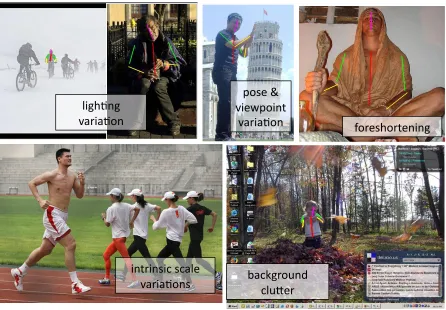
One of the primary difficulties in human pose estimation is that appearance of pose is largely unconstrained, making it highly variable with multiple appearance modes. The following issues are illustrated inFigure 1.2.
Lighting: Images of pose can be taken indoor or outdoor, making not only the mean
intensity of the image variable (signal bias), but also contrast (signal gain). This issue is well studied in computer vision, and to an extent, features have been developed to be invariant to lighting,e.g., HoG (Dalal and Triggs,2005b), but require harsh quantization and local normalization of edge energy information.
Viewpoint and pose: Humans can look very different depending on where they are with
!"#$%&#' ()*")%+&'
,)-.#*+/&0' -!/12*' 3+42'5' ("263+"&7''
()*")%+&' 8+*24$+*72&"&#'
"&7*"&4"-'4-)!2' ()*")%+&4'
Figure 1.2: Some of the perceptual challenges in human pose estimation. Large variations in lighting, pose, viewpoint, foreshortening, relative scale and clutter all work to confound pose estimation. See§1.2.1
Relative scale:We assume our input is a detected person at a rough global scale. However,
we still have a large variation in the scale of parts in two different ways: In any particular person, the ratio of limb lengths may not be consistent; e.g. a baby’s proportions are very different than an adult’s. Across people, there are also a large differences in the geometries of parts, based on gender, body type (fat, skinny, muscular), and age. These further contribute to the variability in appearance.
2D projection: The fact that we are working with images that are projections of the real
!"#$ !%#$ !&#$ !'#$
Figure 1.3: Some illustrations of variation in appearance in the PASCAL Stickmen dataset. (a) An average of the dataset in grayscale. (b) Average of Sobel edges over dataset. (c) Polar histogram of the inner angle made between upper and lower arm, with examples for
0◦,45◦,90◦,135◦,180◦,225◦,270◦ and315◦. (d) A random sampling of 100 left elbows from the Buffy Stickmen pose dataset, removing color and intensity bias, to illustrate the huge variety of appearance due to clutter, motion blur, clothing, body type, and pose.
foreground occlusions make a part invisible and are very hard to determine without further scene or depth knowledge. Finally, it is inherently ambiguous to map from 2D pose to 3D real world coordinates (even up to an unknown global scale factor), discussed further in§3.2. This makes it difficult to model priors on arm length, as we are forced to measure and reason about lengths on the 2D pixel grid.
Clothing: Clothing contributes a near-infinite space of foreground variation. Not only is
clothing responsible for foreground clutter, it also can be considered an occluder which hides parts (e.g. baggy clothing, skirts, ponchos) and can break assumptions about left-right appearance symmetry (e.g. an asymmetric shirt).
Background clutter: Background clutter accounts for roughly half the errors in pose
1.2.2
Computational issues
To operationalize Problem 1, let x be the input image pixels, and y be a representation of the output predicted pose. Then a general solution toProblem 1 would take the form of a scoring function s(x, y) which evaluates the quality of any estimated posey in the image x. We can define the “best” pose as the highest scoring: y? = arg max
ys(x, y)
(ory? = arg sup
ys(x, y)ify is infinite dimensional,i.e. continuous). ThenProblem 1is
satisfied if this determination of the maximizer can be done in polynomial time. There are two sources of intrinsic computational complexity within this framework.
Complexity of the input: For the reasons outlined in §1.2.1, there are an astronomical
number of different inputsxthat can map to the same true posey—the same layout of body parts can look very different from image to image. The problem is inherently multimodal, in the sense that radically different appearances are equally valid input representations of any particular pose. For a few different illustrations of the variability of a dataset,
seeFigure 1.3.
To deal with this complex problem, we are forced to either design features that are invariant to the multimodality (e.g., a generic patch-based arm detector based on coarse edges, or geometric features based on relative part coordinate systems), or to partition the space and model multiple modes separately. In the case of the latter approach, we are faced with other difficult decisions regarding model complexity: how to define modes and a notion of locality, and what the right trade-off is between the richness of the model and the error in fitting the model at different modes with a finite amount of training data.
Complexity of the output:The enormous combinatorial space of possible output poses is
a second source of computational complexity. A typical discretization of the state space of human poses is an80×80spatial grid of part locations at24possible angles (Felzenszwalb and Huttenlocher, 2005), resulting in an output space that is roughly150000possibilities for each part, and thus 1500006 ≈ 1030 for the joint output space of all 6 upper body
parts1.
Enumerating all possibilities for a joint configuration of all parts is clearly not feasible. At the other extreme, we could ignore part interactions, and estimate the pose of each part separately—a task which instead has 6×150000possibilities, which is computationally very cheap with modern computers. However, individual part detection is extremely diffi-cult for body parts (Andriluka et al.,2009) due to the wide range of appearances and lack of discriminating features.
Between the two extremes of (1) estimating parts in isolation and (2) enumerating all possible joint pose configurations, there lies a family of modelss(x, y)that considersome
part interactions, but not all. The simplest of these is a first-order, or pairwise model, which looks at pairs of part interactions at a time, and the graph of part interactions forms a tree structure. This compromise between a full model of every part and a decoupled model of independent parts will be the basic model building block throughout this work.
In such a pairwise model, the basic bottleneck operation is to evaluate the quality of a pair of parts at a time. The model combines all such pairwise scores together to determine the optimal global pose. This scoring requires1500002 ≈1billion possibilities to consider for a pair of parts in our example80×80×24state space, which is large but just small enough for modern machines to handle with some additional model restrictions, detailed in§3.
1.3
Contributions of this thesis
Due to the computational issues discussed above, previous work in pose estimation has resorted to a model of pose that considers, at most, pairwise interactions between parts, in a specially restricted form: the network of part-pair interactions is described by a tree structured graph, and the interactions are described by simple kinematic consistency. This is known as the basicpictorial structure(PS) model, also referred to as aspring model— see§3, andFigure 1.5.
!"#$%&!"#$%$"#$"&'
'#!()!*%+*,-(%*+
!"#$%&#$%$"#$"&'
'#!()!*%+*,-(%*+
Figure 1.4: Puzzle analogy of pose estimation. Classical approaches only use individual part detectors and geometric plausibility to determine the pose of a person. This is anal-ogous to attempting to put together a puzzle without looking at appearance of the pieces —only the plausibility of them fitting together. On the other hand, models with data-dependent interactions are analogous to using the appearance of the puzzle piece faces as well as their fit when constructing the puzzle. Even for humans, it is easier to spot the correct pair of upper/lower arms when they are examined jointly.
Figure 1.5: Spring model of pose. At left, the original spring pictorial structure model that appeared in Fischler and Elschlager(1973). At right, the standard PS model for 2D human pose. The states are shown as unit vectors indicating the position of joints and their direction. The mean displacement between joints are shown as solid black circles, connected by solid black lines to show the kinematic tree structure. The displacement from mean positions are shown as springs stretching. This figure is repeated again for convenience in§3.
beliefs and respecting the prior notion of what a pose should look like.
An important property of PS models is that the pairwise, spring stretch, termsareblind to the image content. The problem with this is that individual part detector scores are extremely weak (§1.2.1): they must work in isolation and generalize to limbs in all settings of backgrounds, foregrounds, articulation, and environment.
one can only see how well they fit together, andnot the image content on their faces; see
Figure 1.4-top row.
1.3.1
Image-dependent interactions in a tree structured model,
§
5
As an improvement over the basic PS model, we wish to actuallyexploit image content when modeling pairwise interactions. In the puzzle analogy, this would allow us to fit pieces together based on their color similarity and continuous contours across the connec-tion boundary; seeFigure 1.4-bottom row. We exploit these same cues for determining whether limbs go together in an image, as well as additional cues such as region support and multimodal descriptions of geometry.
Unfortunately, this turns out to be computationally infeasible using standard tools and techniques. In light of this, we propose a cascade of models to focus computation on pose possibilities that are more promising. There are many pose possibilities that are easy to reject as incorrect with a simple model (like a basic PS model, or even simpler), and we are then able to freely apply a richer model on the possibilities that remain. This is illustrated inFigure 5.4.
To employ a cascade approach, we develop and analyze structured prediction cas-cades, and apply them to the problem of 2D pose estimation. Importantly, we provide a novel training objective for the cascade so that parameters of the models are learned to specifically to filter out a significant proportion of possibilities at every cascade level.
1.3.2
Image-dependent interactions in a general graph,
§
6
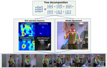
over a general cyclic graph of part relationships is known to be #P-hard (Koller and Friedman,2009)—exponential in the number of frames of video. We provide an
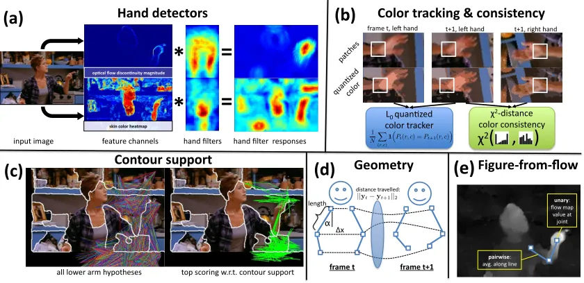
approx-imate approach which decomposes a cyclic model of pose into a collection of subgraph trees, whose union of edges covers all the relationships we care to model. This allows us to exploit all the interesting interaction terms in the original model with efficient inference in each subtree, thanks to the structure and the use of our cascade approach. Then, we can exploit all cues used in the tree-based model, and in addition, cues based on color sym-metry across the body, and temporal appearance and location persistence information. We propose and investigate empirically different methods of reaching a consensus between the subtrees.
We evaluate our approach on a new video dataset, the first of its kind in tracking human pose in the wild without any assumed extra knowledge. We show our proposed model and approximation scheme is beneficial, beating the state-of-the-art in pose estimation systems.
1.3.3
Multimodal interactions,
§
7
The aforementioned models focus attention on increasing the quality of features and in-creasing the number of modeled part interactions. The hope is that these more expressive models do a better job at capturing the inherently multimodal appearance space of poses, by better separating the true pose configurations from false alarms. This somewhat ad-dresses the issue of non-linearity in lower-dimensional feature spaces, e.g., using only edge information.
for,e.g., an arms crossed mode, an arms raised mode, etcetera.
1.3.4
Technical summary of models
This section is intended for readers who already have an understanding of pairwise struc-tured models and the parts-based pose estimation literature. It provides a quick overview of the model formulations discussed in depth in the rest of this thesis. It does not give a self-contained explanation, and the unfamiliar reader is encouraged to skip this section.
The basic pictorial structure model takes the form
s(x, y) = X i∈VΥ
φi(x, yi) +
X
i,j∈EΥ
φij(yi−yj)
where the network of part pairwise interactions is described by a tree structured graph
Υ = (VΥ,EΥ). The first termsφi(x, yi)score how likely a part is to be placed at
loca-tionyi, independent of other parts. The pairwise termsφij(yi −yj) score the geometric
compatibility between pairs of parts. Importantly, this pairwise term isblind to the image content.
Instead, we wish to actually exploit image content when modeling pairwise interac-tions. To this effect, in§5we propose a more general model of human pose, of the form
s(x, y) = X i∈VΥ
φi(x, yi) +
X
i,j∈EΥ
φij(x, yi, yj) (1.1)
The model we propose Equation 1.1works for any tree-structured model, but cannot be applied to cyclic models. We address this with a generalization ofEquation 1.1:
s(x, y) = X i∈VG
φi(x, yi) +
X
i,j∈EG
φij(x, yi, yj) (1.2)
where G = (VG,EG) is a general graph, not just a tree. Determining the best possible
answer arg maxys(x, y) over a general graph G is known to be #P-hard (Koller and Friedman,2009)—exponential in the number of frames of video. To deal with this, we
ex-plore state-of-the-art approximation techniques, such as dual decomposition, and propose a simpler approximation technique the performs at least as well with orders of magnitude less computation. See§6.
The aforementioned models focus attention on increasing the quality of features and increasing the number of modeled part interactions. The hope is that these more expres-sive models do a better job at capturing the inherently multimodal appearance space of poses, by better separating the true pose configurations from false alarms. This somewhat addresses the issue of non-linearity in lower-dimensional feature spaces, e.g., using only edge information.
Complementary to the models described by Equation 1.1and Equation 1.2, in§7we propose to capture this nonlinearity directly as follows:
s(x, y, z) = X i∈VG
φi(x, yi, z) +
X
i,j∈EG
φij(x, yi, yj, z) (1.3)
where now the goal is to determine not only the best pose layouty, but also whichmodez
the pose belongs to:y?, z? = arg max
y,zs(x, y, z). Each mode need only model a portion
1.3.5
Summary of contributions
In summary, the work detailed in this thesis contributes the following to the fields of machine learning and computer vision, and especially their intersection for human pose estimation:
• New models of human pose that capture image-dependent interactions.
• Computational innovations that enable learning and inference in these models, which are na¨ıvely intractable: structured cascades and tree ensemble methods.
• A variety of new features and feature types not typically applied to pose estimation. Some of these are bottom-up type features complementary to the traditional edge-based cues.
• State-of-the-art results on the public Buffy and Pascal Stickmen single frame datasets,
and our introduced MoviePose single frame and VideoPose video sequence datasets.
1.3.6
Published work supporting this thesis
Part I
Chapter 2
Structured Prediction
In this section we lay out the basic definitions and tools necessary for data-driven modeling ofclassification problems. In the most general setting, the goal is to learn a mapping, or
classifier, h in a hypothesis class H from a set of input examples x to a set of discrete output variables y. We concern ourselves in this work with a specific setting: xlies in a (possibly high-dimensional) vector space (most commonly in this work, the input image pixels) and the target lies in a discreten-dimensional space:
y∈ {0,1, . . . , k}n,Y.
We will refer to the setY ={0,1, . . . , k}nas the set of labels,label set, orstate space
for a dimension ofy. Theithdimension ofywill be indexedyi, and referred to asvariable i. We refer to the state space of partiasYi, and the size of the state space as|Yi|. The size
of the full state space is|Y|=|Y1×. . .× Yn|, where here×denotes a Cartesian product.
For example, in a simple image classification task to determine whether an image has a dog in it, x could be an image’s pixels, and y ∈ {dog, not dog} ∼= {0,1}; an instance of binary classification. In this case,k = 2 and n = 1. In multiclass classifi-cation, k > 2andn = 1, e.g., predicting the handwritten digits0, . . . ,9or the weather
We will discuss four major components necessary for learning and applying machine learning classifiers in this chapter:
• Aninference procedureto determine the most likely label for a fixed test example
x:
h(x),arg max
y∈Y
h(x, y). (2.1)
• Thehypothesis classHfrom which to obtain our classifierh.
• Alearning loss functionL(·)which assesses the quality of any particular classifier
h∈ H.
• Alearning algorithmto find the minimizer ofL:
h= arg min
h0∈H L
(h0). (2.2)
2.1
Generalized linear classifiers
There are many possible parametric and non-parametric choices of hypothesis classesH to consider. One of the easiest to represent, learn, visualize and analyze is the hypothesis class ofgeneralized linear models, of the form
h(x, y) = d
X
i=1
wifi(x, y) =w·f(x, y) (2.3)
wherew∈ Rdis a vector of linear parameters of our model andf(x, y)∈
Rdis a vector
of features that depend on the input and output variables. Thus the model is simply a weighted sum of features to obtain a real-valued score, andH =Rd.
2.1.1
Binary and multi-class classifiers
f1(x) f2(x)
w
f1(x)
f2(x)
w1
w2
y
= 0
y
= 1
w· f(x)
>0
w·f
(x) <0
w0
y
= 0
y
= 1
y
= 2
!"#$%&'()$**"+($,-#' ./),0()$**'()$**"+($,-#'
Figure 2.1: Binary and multi-class classification. On the left is shown a binary labeling problem in 2 dimensions, with a linear classifier which perfectly classifies the data. On the right is shown a 3 class classification problem, with a linear classifier for each class, each of which perfectly separates the correct label from the two incorrect labels.
classifiers describe a line, in three dimensions, they describe a plane, and in general, they describe a hyperplanewhich partitions the feature space (for a particular label) into two halfspaces.
Observe that for binary classification, we need only look at which side of a hyperplane a point lies on in a particular feature space to determine the label:
h(x) =1(h(x,1)> h(x,0)) (2.4)
=1(w·f(x,1)>w·f(x,0)) (2.5)
=w·(f(x,1)−f(x,0))>0 (2.6)
=w·f(x)˜ >0 (2.7)
The vector w describes a hyperplane via its surface normal. The test w·f(x)˜ > 0
spaces and interpret the linear classifier askseparating hyperplanes inddimensions, one hyperplane to separate each label from the rest. Figure 2.1-right illustrates an example withk = 3andd= 2.
2.2
Pairwise structured models
In structured prediction, the output space |Y| = |{0, . . . , k}n| is exponential in n and typically enormous. Due to computational and modeling considerations to be discussed, we assume that the full modelw·f(x, y)decomposesintofactors, orcliqueswhich involve overlapping sets of variables:
w·f(x, y) = X
c∈C
wc·fc(x, yc) =
X
c∈C
φc(x, yc), (2.8)
where we use the shorthand for factors φc(·) , wc·f(·). The index c represents a set
of components of y and f, e.g., yc = {y1, y2, y3}. The set C is the set of all factors c
in our model. We can encode the sets of factors and their overlap relations in general using a factor graph(Koller and Friedman, 2009). The number of different settings and representations for structured models is vast and varied and most are outside the scope of this work.
For our purposes, we focus on structured problems with at most pairwise structure, where |c| ≤ 2 ∀c ∈ C1. We can represent a pairwise structured model as a graph G= (VG,EG)where each variableyicorresponds to a vertex in the graph’s vertex setVG,
and each edge inEGcorresponds to two variablesyi, yjbeing involved in a pairwise factor
1This simplification does not result in loss of generality, as factors involving 3 or more variables can
always be converted into pairwise or unary factors with an expanded label set consisting of the Cartesian product of each variable’s state space. For example, a factor involving the variables y1, y2 andy3 with
state space{1, . . . , k}3can be converted into a single variabley
123 ∈ {1, . . . , k3}. This transformation is,
! " # $ %&'()* )&+,(* '(+'-)* xt ./0/1* ./20/21* al ec el er ce le re !b ca la le ra bc bl br b h u c f l r a e k r u z c l r a e f g n o p !"#$ !%#$ x y !"#$ !%#$ 345*(6*&%7*89:;//* !&#$ <(&=* 6-)'-* %5&)>* )5&)>* %%&)>* )%&)>* !'#$ !(#$
Figure 2.2: MRF examples. (a) A robot localization problem on a 10 ×10 grid. (b) Handwriting recognition. (c) Scene labeling. (d) Human pose estimation. (e) Image denoising. See text for details.
φij. We can then decompose our classifier into the special form
w·f(x, y) = X
i∈VG
wi·f(x, yi) +
X
i,j∈EG
wij ·f(x, yi, yj) (2.9)
= X
i∈VG φi+
X
i,j∈EG
φij. (2.10)
There is a huge amount of research dedicated to models of this form originally stemming from statistical mechanics, where it was first used to determine the spin of particles ar-ranged in a grid. From this perspective,Equation 2.10 describes the log of the energy of the particle system. When given a probabilistic interpretation (as we will see in§2.2.1) this type of model is known as apairwise Markov Random Field(MRF). Because of such historical intuitions as a model for energy, we refer to the different terms aspotentials, and
Equation 2.10as the negative of an energy functionwhich we seek to minimize. Terms
Pairwise MRF examples
Our primary application of interest in this work is human pose estimation, whose modeling as an MRF will be discussed in detail in§3. However, to first give motivation and intuition about how and why to model problems via a pairwise MRF, we present a few vision- and robotics-related examples here.
Wandering robot Imagine we are tracking the location of a robot on a map with 100
locations over 100 time steps as inFigure 2.2-a. We have no idea what the robot’s intent is or where he starts out in the world (the “kidnapped robot” scenario), only that he is restricted to moving adjacent grid positions at each time step (i.e., cannot teleport). We have noisy sensor readings x = [x1, . . . , x100] for every time step. The output y is a
sequence of locations the robot visited in all 100 time steps, one out of Y = 100100 = 101000possibilities. By comparison, the estimated number of atoms in the universe is only
1080. A na¨ıve approach would be to model this as a multi-class problem with101000labels,
and try to directly learn a mappingh(x, y) = w·f(x, y)for all possible y. Importantly, there is a lot ofstructureto this problem, the most obvious being that many outputsyare just not valid, due to the fact that the robot can only move to an adjacent location at each step.
The key insight to be made is the following: knowing where the robot is at time tis tremendously useful for determining the robot’s next location at t + 1—the robot must be somewhere in the vicinity. In addition, knowing where the robot is att−1also helps localize it at t + 1, but with diminishing returns—we now know its previous velocity. Going further into the past, there is increasingly less information to help localize where the robot is at timet+ 1. In general, we can make the simplifying assumption thatgiven the recent past, the future is independent of the distant past. Using this intuition, we can model the problem as achainMRF:
w·f(x, y) =
100 X
t=1
φt(x, yt) +
99 X
t=1
φt,t+1(yt, yt+1) (2.11)
only consider pairwise factors over adjacent time stepsφt,t+1, creating a chain of variable
interactions. The unary potentialsφtcan model the likelihood of being in each grid
loca-tion at timet based on sensor readings, and the pairwise potentials can model how likely it is to transition from any locationytto any locationyt+1.
The pairwise term in such tracking problems is typically represented as a transition matrix. In this robot localization problem the transition matrix would be very sparse, since any location can only transition to adjacent grid locations. It might be comprised of the values{−∞,0}indicating which transitions are or aren’t possible, or more generally, log-probabilities of how likely different transitions are: φt,t+1(yt, yt+1)∝logp(yt+1|yt).
In other structured problems, it also makes sense to make independence assumptions
about which dimensions ofyare assumed dependent on each other and their interactions should be directly modeled. For example:
Handwriting recognition In this problem, the output at each position is which letter of
the alphabet is written given handdrawn letter imagesx(in this problem,k = 26if only considering ‘a’,. . . ,‘z’, or roughly70if considering all alphanumerics plus punctuation). Clearly adjacent letters in a document are highly correlated (e.g., adjacent outputs such as ‘ab’ and ‘he’ are likely, but ‘hb’ is not), but depend very little on letters far away in the word, sentence or even document. Practitioners again typically model this as a chain, seen
Figure 2.2-b.
Scene labeling In scene labeling, the goal is to label coarse segments of an image with
scene types (“sky”,“grass”,“building”,“cow”, etcetera;k is on the order of tens of labels) given the image asx. The typical assumption made is that adjacent regions’ labels directly depend on each other, whereas the label of spatially distant segments have weak or no interactions and are not modeled (Cour et al., 2005). The MRF model thus connects adjacent segments in the image, giving us a cyclic planar graph as inFigure 2.2-c.
Human pose estimation Knowing the location of the left shoulder is a strong cue for
describe the human layout as a tree graph corresponding to the kinematic skeleton, see
Figure 2.2-dand§3.
Image denoisingHere the inputxis an image with a small set of labels that are corrupted
by noise; the goal is to determine the uncorrupted original imageythe same size asx. In this settingk is typically 2 or a small set of indexed colors. Practitioners typically model this problem with a grid graph, where variable y(r,c) corresponds to pixel label at rowr,
columnc, and is in pairwise factors withy(r+1,c), y(r−1,c), y(r,c+1), andy(r,c−1). Pairwise
terms model the assumption that adjacent pixels are likely to have the same label, e.g.,
φ(r,c),(r+1,c) ∝1
y(r,c)=y(r+1,c)
. SeeFigure 2.2-e.
You may object that some of the decomposition assumptions made in the above exam-ples are somewhat extreme. However, they are typically seen as forgivable thanks to the greater simplicity of modeling only local interactions. Even more enticing is the reduction in computation they allow, discussed in§2.3.
2.2.1
Probabilistic interpretation
Much of the development of machine learning models and methods originally came from the probabilistic modeling and statistics literature (Bishop, 2006; Friedman et al., 2001; Koller and Friedman, 2009). From this perspective, our model describes a log-linear
probabilistic form of the posterior probabilityp(y|x):
p(y|x) = P exp [w·f(x, y)]
y∈Yexp [w·f(x, y)]
= 1
Z(x)exp [w·f(x, y)] (2.12)
It can be shown that this particular form of p(y|x)is the distribution with maximum en-tropy, subject to the constraints that feature expectations with respect to p(y|x) match empirical feature expectations in a training set (Jaynes,1963). This principle is based on the desire to have our model make as few assumptions as possible (be most entropic) about the observed data.
and not worry about normalization byZ(x):
arg max y
p(y|x) (2.13)
= arg max y
logp(y|x) (2.14)
= arg max y
w·f(x, y)−logZ(x) (2.15)
= arg maxw·f(x, y) (2.16)
A distributionp(y|x)modeling a structuredythat decomposes over factors as in§2.2
takes the form:
p(y|x)∝exp
" X
i∈VG φi+
X
i,j∈EG φij
#
= Y
i∈VG
expφi
Y
i,j∈EG
expφij (2.17)
Historically and in other settings, terms expφc were assumed to be themselves proper
jointp(yc, x)or posteriorp(yc|x)distributions over subsets of random variablesc, but we
assume no such restriction in our case.
Sometimes people make distinctions between fitting parameters for agenerative model
of the formp(x, y)versus a discriminative modelof the form by referring to the former as a Markov Random Field, and the latter as aConditional Random Field(CRF) (Lafferty et al.,2001) orDiscriminative Random Field(Kumar and Hebert,2003). The differences between MRFs and CRFs lie in the way in which models of the formEquation 2.17are trained, and restrictions on the form of the potentials allowed.
In all our work, we assume no restrictions on the form of potentials, always assume
x is given and y is to be estimated, and learn a discriminative model, like a CRF (see
2.3
Inference
The inference problem is to determine the highest scoring possibility out of all possible outputs inY:
y? =h(x) = arg max y∈Y
h(x, y). (2.18)
We use the convention h to mean hypothesis or hypothesis class, originating from the machine learning community. In the spirit of optimization, we also view this as ascoring functionand use the synonymous notationsto denote the score:
s(x, y),h(x, y) (2.19)
When Y is low-dimensional, brute-force search is easy enough: evaluate s(x, y)for all possibley, and return the highest scoring. This is possible for both binary and multi-class classification, where we evaluate up tok possible labels to determine the highest scoring. However, in the most general setting, the size ofY is exponential ink: |Y| =kn, and
we can’t hope to enumerate all possible outputs inY to find the highest-scoring. Thank-fully, the decomposable structure we impose on our models, discussed in§2.2, allows us to find a solution time polynomial inkand linear inn.
As a simple example of this, consider our wandering robot problem (§2.2) where we make the common assumption that we only model temporally adjacent pairs of output variables together, making a chain of variable dependencies:
w·f(x, y) =
100 X
t=1
φt(x, yt) +
99 X
t=1
φt,t+1(x, yt, yt+1)
Observe now how computing the maximum score of the classifier also decomposesfor this simple problem:
max
y∈Y w·f(x, y) = maxy1,...,y100
100 X
t=1
φt(x, yt) +
99 X
t=1
φt,t+1(x, yt, yt+1) (2.20)
= max y100
φ99,100+φ100+. . .max y3
φ3,4+φ3+ max
y2
φ2,3+φ2+ max
y1
φ1,2+φ1
. . .
InEquation 2.21, we see that the max over each dimension ofycan be nested and needs only reason over at largest a pairwise factor at a time. In our robot problem, each pairwise factor is only 1002 numbers to consider and each unary factor is of size 100. Thus the
total amount of numbers that need to be examined in this problem is roughly 106, an
astronomical improvement over the complete space of 101000. In general the bottleneck
of inference is the max over the pairwise factors having size k2, and thus inference is O(n·k2).
When an MRF model forms a tree, we can always exploit the structure in a similar way for exact efficient inference (Koller and Friedman,2009). Using the same trick we used in the specific example of the robot localization problemEquation 2.21, we can perform inference by nesting themaxoperator over pairs of variables at a time, as well as storing
the arg max maximizer of each max operation. For completeness, the algorithm is in
Algorithm 1, commonly referred to as max-summessage passing, belief propagation, or
viterbi decoding. The algorithm results in inference that isO(n·k2)computation rather thankn.
When the MRF interactions do not form a tree, inference becomes #P-hard. For example, if we could determine the maximizer in a loopy MRF, we could in polynomial time transform it to determine how many variable assignments satisfy a given 3-SAT for-mula (Koller and Friedman, 2009; Valiant, 1979). Thus, no known algorithm exists in general for inference that is polynomial in the number of variables. As a sanity check,
Al-gorithm 1breaks down for loopy graphs: we have no topological ordering of the network
for which we can pass belief messages up to a root, and then backtrack in reverse to obtain the best solution.
2.4
Max-marginals
Often we are only interested in the best scoring complete assignmenty? = arg max
ys(x, y)
and its corresponding score s?(x) = max
Algorithm 1: Max-sum message passing to solve
arg max y∈Y
s(x, y) = arg max y∈Y
X
i∈V
φi+
X
ij∈E
φij
Input: Factors{φi},{φij}, tree graphG= (V,E)with (arbitrary) root node indexr
and topological orderingπ, whereπn =r.
Output: y? = arg maxys(x, y)
fori=π1, π2, . . . , πndo mi =φi+Pj∈kids(i)mj→i
ifi==rthen
break
p=parentπ(i)
mi→p = maxyiφip+mi
ai = arg maxyiφip+mi
y?
r = arg maxmr
fori=πn−1, πn−2, . . . ,1do y?i =ai
h
y?parent
π(i)
However, another extremely useful quantity which we rely on often in this work is the no-tion of amarginalscore. When treating our model as a log-linear conditional distribution
p(y|x)(see§2.2.1), we can consider the marginal distribution of a particular variable
p(yi|x) =
X
yjs.t.j6=i
p(y|x) (2.22)
as a measure of the model’s belief over the value of variablei.
Similarly, we explore the notion of amax-marginal, an analogous quantity for themax
operator:
s?x(yi),max y0 s(x, y
0
), subject to: yi0 =yi (2.23)
In words, the max-marginal score foryi is the score of the best full assignment restricted
to fixing variableito beyi.
A na¨ıve way to compute s?x(yi) for all states in our model is as follows: for each i and each yi (in total nk possibilities), set φij(x, yi0, yj) ← −∞ for all yi0 6= yi, and
all j attached to i, then run Algorithm 1. This ensures that yi is the “chosen” state for
variable i, and we get its max-marginal score s?
x(yi). This strategy would cost in total O(nk·nk2) = O(n2k3), which is not very satisfying.
It turns out we can compute max-marginal quantities for allnkvariable-state possibil-ities inO(nk2)time using a forwardand backward pass of message passing and careful
bookkeeping, similar to Algorithm 1. In addition, we can also collect witness statistics, which keep track of the number of times different states have been used in any max-marginal satisfying assignment (and thus are a “witness” to the assignment). Thewitness
fors? x(yi)is
y?(yi),arg max
y0
s(x, y0), subject to: y0i =yi, (2.24)
which is the maximizer which corresponds to maximums?x(yi).
u
�
(
u
)
−
0
3
−
2
−
1
0
1
2
3
5
10
15
20
25
data1
data2
data3
data4
data5
data6
max{0,1−u}
(1−u)2
(max{0,1−u})2
exp(−u)
1(u <0)
log(1 + exp(−u))/log(2)
(0-1 loss)
(log loss)
(exp loss)
(square loss)
(hinge loss)
(square hinge loss)
−3 −2 −1 0 1 2 3
0 0.5 1 1.5 2 2.5 3 3.5 4
Figure 2.3: Convex surrogate supervised loss functions.
2.5
Supervised learning
In the supervised learning setting, we have access to a training setS ={(x(j), y(j))}mj=1of examples assumed to be sampled independently, identically distributed (i.i.d.) from some true joint distribution(x, y)∼P(X, Y). The standard supervised learning task is to learn a hypothesish:X × Y 7→ Ythat minimizes the average misclassification error (0/1 error) on the training set:
L0/1(h, S) =
1 m
m
X
j=1
1 h(x(j))6=y(j) (2.25)
The linear hypothesis class we consider is of the form h(x) = arg maxyh(x, y), where the scoring functionh(x, y),w·f(x, y)is the inner product of a vector of parametersw
and a feature functionf :X×Y 7→Rdmapping(x, y)pairs todreal-valued features, as
discussed in§2.1.
model from training data:
minimize
w L0/1(h, S) = (2.26)
minimize w 1 m m X j=1 1 arg max y
[w·f(x(j), y)]6=y(j)
(2.27)
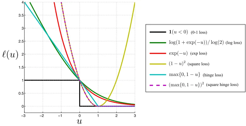
The above optimization is extremely difficult to solve in high dimensions because it is non-convex and discontinuous, leading to many poor local minima. In light of this, we introduce a convex surrogate to the indicator loss function `(·) to replace 1(·) with an upper-bound (Bishop,2006):
minimize
w L`(h, S) = (2.28)
minimize w 1 m m X j=1 ` max
y w·f(x
(j), y), y(j)
(2.29)
There are many common choices for`(·), shown inFigure 2.3, leading to many different structured and non-structured machine learning algorithms. We choose to use the hinge loss for most of this work, which leads to a simple and intuitive stochastic optimization algorithm. The hinge loss is of the form`(u) = max(0,1−u), [1−u]+, giving us the
following optimization problem:
minimize w 1 m m X j=1 max
y w·f(x
(j), y)−w·f(x, y(j)) + 1
+
(2.30)
Depending on the training set, this form of learning function may have issues. Particularly, if the training set isseparable, there are many possiblew’s that will achieve an optimum value of0in Equation 2.30. For example, if awis a minimizer, so is 10·w. Thus, we add an additional regularization term that seeks to find a low errorw, as well as a simple
w—one whose weights are small. To this effect, a regularized form is
minimize
w
λ
2||w||
2 2+ 1 m m X j=1 max
y w·f(x (j), y)
−w·f(x, y(j)) + 1
+
(2.31)
which encourageswto be small in anL2-norm sense. The meta-parameterλbalances how
Model simplicity implies a better chance of generalizing to new data, at the risk of being too restrained to learn an effective classifier. Such concerns about model underfitting or overfitting and the tradeoff between model bias and model variance are well-studied in the machine learning literature, especially for linear classifiers. SeeBishop(2006);Friedman et al.(2001) for rigorous treatments.
2.5.1
Learning algorithms
Any convex learning function of the form of Equation 2.29 lends itself to a variety of optimization algorithms. Because we are guaranteed to reach a global optimum (modulo numerical precision and computational limitations), we focus on choosing a method that is quick and simple. Stochastic first-order descent methods estimate the gradient of the function one data point at a time, and are attractive due to their low memory requirements and fast convergence rates per example examined (Shalev-Shwartz et al.,2007).
UsingEquation 2.31, the second term is piecewise-linear, and we take stochastic sub-gradient steps to optimize it, also known as structured perceptron (Collins,2002). Given a single supervised example(x, y), we make the following update if the second, hinge loss term ofEquation 2.31(i.e., the subgradient) is non-zero:
w0 ←(1−ηλ)w+η(f(x, y)−f(x, y?)). (2.32)
Chapter 3
Pictorial structures:
Pose estimation meets structured
prediction
Classical pictorial structure models (PS models) are a class of structured models specifi-cally proposed to represent 2D objects with parts which can articulate in a kinematispecifi-cally plausible way. The model was first proposed byFischler and Elschlager(1973), and has been hugely popular in computer vision since computational innovations byFelzenszwalb and Huttenlocher(2005).
Pictorial structures take the form of a pairwise structured model as described in§2.2:
s(x, y) = X i∈VG
φi(x, yi) +
X
ij∈EG
φij(yi−yj) (3.1)
with the important exception thatthe pairwise termsφij(yi−yj)are image-independent—
they are not a function ofx.
one way to think about the representation for each part is a unit vector describing position and orientation of each limb, and the state space as a 3D cuboid.
Edge structure: In order to support tractable inference, the part interaction structure
G must be a tree (§2.3). The most common tree is formed by considering kinematic connections only: the lower-arm is connected to the upper-arm, the upper-arm to the torso, etcetera.
Unary potentials: The unary potentials φi(x, yi) encode how likely a limb is at
loca-tion/orientationyi in the image. This can be thought of as a part detector applied to an
image patch located at yi. In practice these detectors are patch-based sliding window
object detectors, applied at every location and orientation. The typical representation is based on edge information in order to be invariant to lighting and color. Edge orientation and magnitude are often locally quantized and histogrammed to be more numerically and spatially stable, and invariant to local signal gain. Feature representations are discussed in detail in§8.
Pairwise potentials: Pictorial structures assumes a restricted form of pairwise potential
the depends only on the deformation between kinematially attached parts. In general, this is a quadratic stretching cost of the form
φij(yi−yj) = −||Tijyi−Tjiyj −δij||22 (3.2)
whereTij are rigid transformations (rotation, translation and scale) to place neighboring
parts in a local coordinate frame, andδij is the expected displacement between the parts.
For example, φij(yluarm − yllarm) measures the squared Euclidean distance between the
elbow locations according to the left upper arm and left lower arm variables.
Spring model interpretation: The reasons for restricting the pairwise potential to be
only a function of spatial deformation are primarily computational, as discussed in§3.1. In addition, this type of model is simple and intuitive to interpret as a “spring model” of object layout: the PS model can be interpreted as a set of springs at rest in default positions
δij stretched by displacementTijyi −Tjiyj. The spring tightness is encoded by warping
Figure 3.1: Spring model of pose. At left, the original spring pictorial structure model that appeared in Fischler and Elschlager(1973). At right, the standard PS model for 2D human pose. The states are shown as unit vectors indicating the position of joints and their direction. The mean displacement between joints are shown as solid black circles, connected by solid black lines to show the kinematic tree structure. The displacement from mean positions are shown as springs stretching.
space. The unary terms pull the spring ends towards locations yi with higher scores φi
which are more likely to be a location for parti. Thus the spring model seeks a balance between confidence in individual part detectors, and the amount of deformation from a default, 2D geometric prior of the human layout. Figure 3.1provides an illustration.
3.1
Sub-quadratic inference
As discussed in§2.2, the computation required to obtain the highest-scoring pose out of the exponentially-many possibilities according toEquation 3.1isO(kn2), usingAlgorithm 1.
checking all such possibilities. Doing this for all left or right upper arms yields an exact
n2 local search.
In practice, there is no need to checkallpossibilities of lower arms for each upper arm location; it is sufficient to check only in a reasonable spatial window around the mean dis-placement locationδij, because it is impossible for kinematically-connected object parts
to be stretched too far. Even so, we must search over a fixed fraction of neighbor states for each part, which still scales quadratically with the resolution of the state space. Typically a state space window of80/5×80/5×24possibilities need to be evaluated for each loca-tion, yielding on the order of(80×80×24)2/25 = 943,718,400computations—nearly a billion—for a pair of parts.
The search operation described here is exactly that performed in the following lines of
Algorithm 1, whereiindexes a part, andj its parent in a topological ordering of the tree
graph1:
mi→j = max
yi
φij +mi (3.3)
ai = arg max
yi
φij +mi (3.4)
The quantity ai(yj) is the best placement of part i when placing part j at location yj,
using all the information from predecessor parts in the topological ordering. The quantity
mi→j(yj)is the corresponding score for that placement.
It turns out that when the pairwise termφij takes the form it does for classical PS, then
we can apply a generalized distance transform procedure to compute ai and mi→j over
all possibilities for yi andyj in time linear in the number of states. This makes the total
cost of inference O(kn) instead of O(kn2). This was introduced by Felzenszwalb and Huttenlocher(2005).
The generalized distance transform solves the problem
Dq(p;f) = min
q ||p−q|| 2
2+f(q) (3.5)