University of Pennsylvania
ScholarlyCommons
Publicly Accessible Penn Dissertations
1-1-2016
Sequential Learning and Variable Length Markov
Chains
Joshua Magarick
University of Pennsylvania, [email protected]
Follow this and additional works at:
http://repository.upenn.edu/edissertations
Part of the
Statistics and Probability Commons
This paper is posted at ScholarlyCommons.http://repository.upenn.edu/edissertations/1870
For more information, please [email protected].
Recommended Citation
Magarick, Joshua, "Sequential Learning and Variable Length Markov Chains" (2016).Publicly Accessible Penn Dissertations. 1870.
Sequential Learning and Variable Length Markov Chains
Abstract
Sequential Learning is a framework that was created for statistical learning problems where $(Y_t)$, the sequence of states is dependent. More specifically, when it has a dependence structure that can be represented as a first order Markov chain. It works by first taking nonsequential probability estimates $P(Y_t | X_t)$ and then modifying these with the sequential part to produce $P(Y_t | X_{1:T})$. However, not all sequential models on a discrete space admit such a representation, at least not easily. As such, our first task is to extend Variable Length Markov Chains (VLMCs), which belie their name and are not Markovian, to be used in the sequential learning framework. This extension greatly broadens the scope of sequential learning as using VLMCs permits sequential learning with far fewer assumptions about the underlying dependence of states. After developing the VLMC extension we provide an overview of sequential learning in general and
investigate the probability estimates it produces both theoretically and with a simulation study to assess model performance as a function of the complexity of the underlying sequential model and the quality of the initial probability estimates. Next, we apply VLMC sequential learning to the original dataset and problem that inspired sequential learning --- that of scoring sleep in mice using video data. We find that VLMCs perform at the same level, tying and sometimes beating the previous best sequential method which required many assumptions about the sequence of sleep states and a much more rigid model of sequential dependence. Finally, we turn our attention to the problem of modifying predictors when marginal class probabilities are known. This is inspired by the fact that in sequential learning problems, the marginal class distribution can vary substantially from sample to sample in contrast to i.i.d. problems. We provide a general method of marginal probability reweighting, show it to be equivalent to several extant methods used on similar problems, and provide a proof that our method improves probability estimates under log loss. We conclude with
simulations assessing our method as a function of loss type and classifier used.
Degree Type
Dissertation
Degree Name
Doctor of Philosophy (PhD)
Graduate Group
Statistics
First Advisor
Abraham J. Wyner
Subject Categories
SEQUENTIAL LEARNING AND VARIABLE LENGTH MARKOV CHAINS
Joshua M. Magarick
A DISSERTATION
in
Statistics
For the Graduate Group in Managerial Science and Applied Economics
Presented to the Faculties of the University of Pennsylvania
in
Partial Fulfillment of the Requirements for the
Degree of Doctor of Philosophy
2016
Supervisor of Dissertation
Abraham J. Wyner, Professor of Statistics
Graduate Group Chairperson
Catherine M. Schrand, Professor of Accounting
Dissertation Committee
Abraham J. Wyner, Professor of Statistics
Dean P. Foster, Professor of Statistics
SEQUENTIAL LEARNING AND VARIABLE LENGTH MARKOV CHAINS
c
COPYRIGHT
2016
Joshua Mark Magarick
This work is licensed under the
Creative Commons Attribution
NonCommercial-ShareAlike 3.0
License
ACKNOWLEDGEMENT
It is easy to thank people in words, but much harder to do so with actions. Many people
have helped me so far and I’m sure many more will. If I tried to enumerate them all here,
I would likely forget some. And if I could list them all here, what a long, long, list it would
be. To me, it is far more meaningful to make sure they all know personally, and to show
through my actions the magnitude of my gratitude. I hope I can do at least as much for
ABSTRACT
SEQUENTIAL LEARNING AND VARIABLE LENGTH MARKOV CHAINS
Joshua M. Magarick
Abraham J. Wyner
Sequential Learning is a framework that was created for statistical learning problems where
(Yt), the sequence of states is dependent. More specifically, when it has a dependence
structure that can be represented as a first order Markov chain. It works by first taking
nonsequential probability estimatesP(Yt|Xt) and then modifying these with the sequential
part to produceP(Yt|X1:T). However, not all sequential models on a discrete space admit
such a representation, at least not easily. As such, our first task is to extend Variable Length
Markov Chains (VLMCs), which belie their name and are not Markovian, to be used in
the sequential learning framework. This extension greatly broadens the scope of sequential
learning as using VLMCs permits sequential learning with far fewer assumptions about
the underlying dependence of states. After developing the VLMC extension we provide
an overview of sequential learning in general and investigate the probability estimates it
produces both theoretically and with a simulation study to assess model performance as a
function of the complexity of the underlying sequential model and the quality of the initial
probability estimates. Next, we apply VLMC sequential learning to the original dataset and
problem that inspired sequential learning — that of scoring sleep in mice using video data.
We find that VLMCs perform at the same level, tying and sometimes beating the previous
best sequential method which required many assumptions about the sequence of sleep states
and a much more rigid model of sequential dependence. Finally, we turn our attention to
the problem of modifying predictors when marginal class probabilities are known. This is
inspired by the fact that in sequential learning problems, the marginal class distribution
can vary substantially from sample to sample in contrast to i.i.d. problems. We provide
extant methods used on similar problems, and provide a proof that our method improves
probability estimates under log loss. We conclude with simulations assessing our method
TABLE OF CONTENTS
ACKNOWLEDGEMENT . . . iii
ABSTRACT . . . iv
LIST OF TABLES . . . viii
LIST OF ILLUSTRATIONS . . . x
LIST OF ALGORITHMS . . . xi
CHAPTER 1 : Introduction . . . 1
CHAPTER 2 : Markov Chains to Variable Length Markov Chains . . . 5
2.1 Fixed Order Markov Chains . . . 5
2.2 Semi-Markov Models . . . 6
2.3 Variable Length Markov Chains . . . 10
2.A Appendix: Detailed Context Tree Fitting . . . 19
CHAPTER 3 : Sequential Learning . . . 21
3.1 Hidden Markov Models . . . 21
3.2 Discriminative HMMs . . . 30
3.3 Results on Probability Estimation . . . 32
3.4 VLMC simulations . . . 34
CHAPTER 4 : Application: Mouse Sleep Data . . . 51
4.1 The Data . . . 51
4.2 Analysis . . . 57
CHAPTER 5 : Sequential Learning and Probability Estimation . . . 78
5.1 Original Simulations . . . 78
5.2 Using the Marginal Distribution . . . 87
5.3 Results with Modified Classifiers . . . 90
5.4 Classification with Known Marginals . . . 93
CHAPTER 6 : Conclusion and Future Work . . . 110
6.1 Future Work . . . 111
LIST OF TABLES
TABLE 1 : Sleep State by Time of Day . . . 57
TABLE 2 : Table of Bout Statistics . . . 59
TABLE 3 : Holdout Misclassification Rates . . . 61
TABLE 4 : Per-Mouse Misclassification Rates . . . 62
TABLE 5 : Holdout REM Performance by Method . . . 73
TABLE 6 : Per-Mouse REM Performance by Method . . . 74
TABLE 7 : Two State Holdout Misclassification . . . 75
TABLE 8 : Two State Per-Mouse Misclassification . . . 75
TABLE 9 : Fit Bout Statistics . . . 76
TABLE 10 : Length 1 Wake Bout Error Rates . . . 77
LIST OF ILLUSTRATIONS
FIGURE 1 : Sequentially dependent data. . . 1
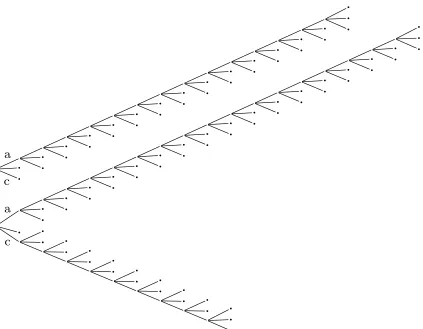
FIGURE 2 : Example Context Tree . . . 15
FIGURE 3 : VLMC Expansion . . . 17
FIGURE 4 : Simulation tree transition probabilities . . . 35
FIGURE 5 : Simulation Trees . . . 36
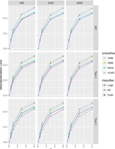
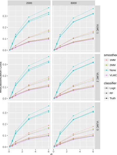
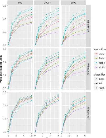
FIGURE 6 : First Simulation Group Misclassification . . . 39
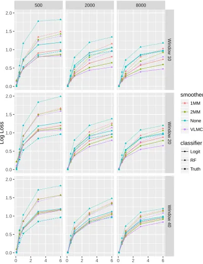
FIGURE 7 : First Simulation Group Log Loss . . . 40
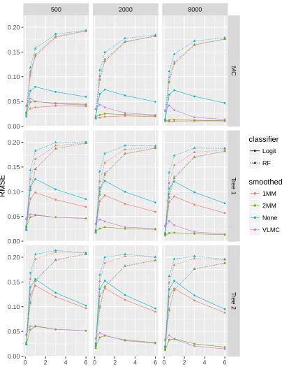
FIGURE 8 : First Simulation Group RMSE . . . 41
FIGURE 9 : Second Simulation Group Misclassification . . . 44
FIGURE 10 : Second Simulation Group Log Loss . . . 45
FIGURE 11 : Second Simulation Group RMSE . . . 46
FIGURE 12 : Third Simulation Group Misclassification . . . 48
FIGURE 13 : Third Simulation Group Log Loss . . . 49
FIGURE 14 : Mouse Video Covariates by State . . . 54
FIGURE 15 : Mouse Video Covariates by State and Time . . . 55
FIGURE 16 : Bout Duration by Mouse Violin Plot . . . 58
FIGURE 17 : REM ROC Curves . . . 64
FIGURE 18 : NREM ROC Curves . . . 65
FIGURE 19 : Wake ROC Curves . . . 66
FIGURE 20 : Mouse Pair Calibration Plot . . . 68
FIGURE 21 : Holdout Calibration Plot . . . 69
FIGURE 22 : Probability Estimate Histograms . . . 71
FIGURE 23 : Parameters for GMM simulations. . . 79
FIGURE 25 : GMM Simulation BNBGT Performance . . . 83
FIGURE 26 : GMM Ternary Plots (T = 1000) . . . 85
FIGURE 27 : GMM Ternary Plots (T = 10000) . . . 86
FIGURE 28 : Corrected GMM Simulation Discrete Beta Performance . . . 91
FIGURE 29 : Corrected GMM Simulation BNBGT Performance . . . 94
FIGURE 30 : Simulation Marginal Class Ternary Plot . . . 104
FIGURE 31 : Log Loss Difference . . . 105
FIGURE 32 : Log Loss Ratio . . . 106
FIGURE 33 : Log Loss Comparison . . . 106
FIGURE 34 : Misclassification Difference . . . 107
FIGURE 35 : Misclassification Ratio . . . 108
LIST OF ALGORITHMS
ALGORITHM 1 : Grow Context Tree (high level) . . . 12
ALGORITHM 2 : Prune Context Tree . . . 14
ALGORITHM 3 : Generate Minimal Markov Hull . . . 17
ALGORITHM 4 : Fit VLMC (Detailed) . . . 20
ALGORITHM 5 : Forward Algorithm . . . 25
ALGORITHM 6 : Backward Algorithm . . . 25
ALGORITHM 7 : Viterbi Algorithm . . . 27
ALGORITHM 8 : Baum-Welch Algorithm . . . 28
Chapter 1
Introduction
The objects of study in this dissertation are problems arising in the study of data with
sequentially dependent labels. By this, we mean that in contrast to many machine
learn-ing problems where the covariate-label pairs, (Xt, Yt), t = 1, . . . , T, not independent. We
presume a dependence structure in place determined by dependence among the Ys.
Addi-tionally, the models we consider treat X as being “emitted” from Y, meaning that Xt is
conditionally independent of all otherXs givenYt. This structure is illustrated graphically
in figure 1. As such, the goal is to estimate P(Yt|X1:T) rather than P(Yt|Xt) because
without observing the labels, the entire sequence X1:T carries information about eachYt.
…"
Y
t 1Y
tY
t+1 …"X
t+1X
tX
t 1P
(
X
t|
Y
t)P
(
Y
t+1|
Y
1:t)What we call the “Sequential Learning” framework was introduced in the context of
mod-eling and scoring the sleep stages of mice using video data by McShane et al. [39]. In this
case, we clearly do not believe that whether a mouse is awake, in REM sleep or in non-REM
sleep is independent from time period to time period. It is also reasonable to assume that
the observations Xt at any given time depend only on the current state of the mouse.
However, while the original work provided a general method for any sequential process that
can be embedded in a first order Markov chain, not all such models are easily representable
in this way. The models used, Generalized and Transition Dependent Generalized Markov
Models, are forms of Semi Markov Models that explicitly and parametrically model the
holding times of each state. While these sequential models worked well with the data, they
are parametric models and selecting both the families of holding time distributions and
parameters used required careful inspection of the data and hand-selection of some parts of
the model.
To this end, we want to apply Variable Length Markov Chains (VLMCs) to this problem.
VLMCs belong to the class of tree-based sequential models commonly used in information
theory and data compression and were introduced in the form we use by B¨uhlmann and
Wyner [11]. Instead of modeling a sequence of states as a fixed order Markov chain or
using parametric holding time distributions, VLMCs produce transition probabilities from
a context function that depends on, as the name implies, a variable number of previous
states. Since this history can be long when needed and short when not, VLMCs are able
to parsimoniously model processes with a long memory. This approach generalizes both
higher order and semi-Markov models and would allow sequential learning on more diverse
data without the need to assume the labels come from a particular parametric process.
However, to do so requires that VLMCs be represented as a first order Markov model. And
unfortunately, the standard fitting algorithm for VLMCs produces trees where this is not
possible, so some modification is required. The na¨ıve way of doing this would be to create
purpose of a VLMC as we would end up with an exponentially large model that we sought
to avoid. Instead, we would like a parsimonious model. Chapter 2, in addition to discussing
VLMCs and how they generalize previous Markov models in sequential learning, provides
a way to do this. We present a necessary and sufficient condition for a VLMC to have a
first order embedding that has far fewer additional states than the number required by the
simplistic method, and an algorithm to create it.
Following this, we turn our attention in chapter 3 to the problem of sequential learning.
After reviewing previous work outlining the algorithm for use with any process representable
as a first order Markov chain and any discriminative classifier we investigate the conditional
class probability estimates produced by sequential learning. First, we prove three new
results about the probability estimates sequential learning produces in different edge cases.
While the assumptions are not realistic in practice, they serve to enhance our intuition and
better understand phenomena that we observe in simulations. We conclude this chapter
with a simulation study to better understand the relationship between sequential learning
and the initial, nonsequential classifier used, finding that while sequential methods always
help, a good nonsequential model can sometimes beat a bad one augmented with sequential
learning.
Next, chapter 4 applies VLMC sequential learning to a real dataset consisting of the sleep
states of mice and measured covariates taken from video recordings. As mentioned above,
this is a good setting for the sequential learning paradigm, as there is signal in our covariates
and the labels have clear and complex sequential dependence. Using VLMCs on this data
performs similarly to, and often better than the previous best sequential method which used
a parametric model on holding times and required far more human intervention to fit. This
result is promising as sleep behavior differs across mice both on an individual and a strain
level. VLMCs may allow us to model this behavior for sequential learning without spending
time and effort trying to pick the right family of distributions to model holding times of
on multiple sequences, which allows us to build more accurate and robust models by fitting
on multiple mice and thus dealing with some of the observed mouse-to-mouse variability.
Finally, chapter 5 addresses our largest contribution of improving probability estimates when
the marginal distribution of labels is known. This question arose from a series of sequential
learning simulations with surprising results that we begin the chapter by replicating. They
ask what happens if we know one piece of a model in sequential learning — either the
Markov part of the nonsequential conditional class probabilities, P(Y |X). The initial
results showed that, when measured by RMSE to the true P(Yt|X1:T), a model that
estimated both parts seemed to do worse than one that knew one part or the other. As we
show in an extension to these simulations, they did not correctly use P(Y), the marginal
class distribution and doing so resolves the problem. While the marginals matter little in
standard statistical learning problems — they vary little from sample to sample — complex
Markovian structures on the label yield empirical marginal distributions that can be quite
different each time we simulate.
From this we investigate the general question of known marginals and provide a method
for incorporating this information into any estimate of conditional class probability. Our
problem is related to several others in the literature, and indeed, we are able to show that
our method of marginal probability rescaling is equivalent to several others used to solve
similar problems. In addition, we provide a proof that rescaled probability estimates are
always better than non-rescaled ones and can even show the exact size of the improvement.
Following this, we present simulations of the method using several classifiers and show that,
Chapter 2
Markov Chains to Variable Length
Markov Chains
This chapter discusses Markov chains and some of their generalizations, which we will use
in classification problems where the class labels are assumed to be dependent. The principal
aims of this chapter are to outline the models, and show how generalizations such as the
Variable Length Markov Chain can be represented as a standard Markov chain.
2.1. Fixed Order Markov Chains
2.1.1. First Order Markov Chains
Definition 1. If (Xn) is a stationary sequence of random variables taking values in a
discrete alphabet Awe say that (Xn) has the Markov property if
P Xn
X0:(n−1)
=P(Xn|Xn−1).
for all n.
outcomes forXndepends only onXn−1, meaning we can “forget” anything observed before
that. The Markov property lets us represent a Markov chain concisely in the form of a
transition matrix Awhere Aij =P(Xn=j |Xn−1 =i)
2.1.2. Higher Order Markov Chains
As with first order Markov Chains, we can define a higher order Markov property where we
are allowed to remember more than just the previous state.
Definition 2. A stationary sequence of random variables (Xn) has themth order Markov
property if
P Xn
X0:(n−1)
=P(Xn|Xn−m).
for all n.
As First Order Markov Chains
Any higher order Markov chain can be represented as a first order Markov chain by
consid-ering tuples of states. For instance, with a second order Markov chain, we might define the
new processX0
t= (Xt−1, Xt), which now exists overA2 - the set of sequences of length two
of elements in A. We would now have a |A|2 × |A|2 transition matrix with |A|3 nonzero
entries, since each state of the new process (Xt0) only has |A|valid transitions.
Higher order Markov models allow for more complicated dependence relationships within
the sequence, but can be problematic in practice. This comes from the fact that there are
|A|m possible previous states the process can be in, meaning there are |A|m+1 transitions
of interest. This means that we would need exponentially more data to fit such models as
as we raise the order of the chain.
2.2. Semi-Markov Models
Sometimes we would like to model a more complex process with longer memory, but either
in some additional assumptions. One such class of assumptions is that the holding times
of states — the number of time steps the chain spends in a state before exiting — follow
some parametric distribution. To see why this is reasonable, consider the holding time for
a first order Markov chain. We have
P(Xt+1=a, . . . Xt+m−1=a, Xt+m 6=a|Xt=a, Xt−1 6=a)
=P(Xt+1=a, . . . Xt+m−1 =a, Xt+m 6=a|Xt=a)
=P(Xt+m6=a|Xt+m−1 =a)
m Y
k=1
P(Xt+k=a|Xt+k−1 =a)
= (P(X2=a|X1 =a))m(1−P(X2 =a|X1 =a))
which is a geometric distribution.
To resolve some issues in modeling higher order Markov process, one method has been to
use Semi-Markov Models [48, 64], also known as Explicit Duration Markov Models[18], or
Generalized Markov Models[38]. This class of models generalizes Markov chains by allowing
states to have non-geometric holding times.
With a Markov chain, the transition matrix A governs the entirety of the process but a
GMM adds the additional component of holding time distributions dj for each j ∈ A.
What this means is that when the process enters state a it also decides how long it will
stay by samplingδ ∼da. So, if our observed sequence isaaabbacccc, then the sequence of
states isabac and the sequence of times is 3 2 1 4. This way of thinking about a process
is considering it as a run length encoding.
Thinking about GMMs like this is fine from a generative point of view, but if the holding
time distributions are not geometric we need to make some modifications to represent this
as if it were a first order model; i.e. with only a transition matrix. To start we will assume
that the da have finite support, that is dj(i) = 0 for i > Mj for someMj for each j.
state pairs Zt = (δt, Xt) where δt is the value of the “clock” at time t and Xt is again the
state of the process. That is, the sequence above would be written as
(3, a) (2, a) (1, a) (2, b) (1, b) (1, a) (4, a) (3, a) (2, a) (1, a).
With this representation, we have P(Zt+1= (i−1, j)|Zt−1 = (i, j)) = 1 for i >1. When
i= 1, Xt+1 must enter a different state and the countdown clock will reset.
When i= 1 we can compute
P(Zt+1 = (i, k)|Zt−1 = (1, j)) =P(δt+1=i, Xt+1=k|Zt−1= (1, j))
=P(δt+1=i|Xt+1 =k)P(Xt+1 =k|Zt−1 = (1, j))
=dk(i)Ajk
Note that in the second line we have used the fact that
P(δt+1=i|Zt−1= (1, j), Xt+1=k) =P(δt+1 =i|Xt+1=k)
because the holding time for the next state is independent of the previous state. As long
as all the dk have finite support, we can see that we now have a first order Markov chain
defined on (Zt). Of course, in principledkcould be an unbounded distribution, but then our
chain would have infinitely many states. One way to handle this is to introduce a special
state ‘+’ to the clock, calling the resulting models “GMM+”, as was done in McShane et al.
[39] where we allow
P(Zt+1= (+, j)|Zt−1 = (+, j)) =pj >0, P(Zt+1 = (Mj, j)|Zt−1 = (+, j)) = 1−pj
parameterpj. The overall holding time distribution for state j upon entry is
dj(i) =qjfj(i)1i≤Mj + (1−qj)gj(i−Mj)1Mj<i
where qj is the probability of ending up in the “head” distribution as opposed to the
geometric “tail” whose pmf is given by gj. Also, fj is a proper PMF defined on 1, . . . , Mj;
so this represents the probability of the clock taking on a certain value given that we end
up in the head part of the distribution. To represent these as first order Markov chains, we
simply note that
P(Zt+1= (i, k)|Zt−1= (1, j)) =qkfk(i)Ajk when i≤Mk
P(Zt+1= (+, k)|Zt−1= (1, j)) = (1−qk)Ajk
Transition Dependent GMMs
We end this section with a brief discussion of Transition Dependent GMMs (TDGMM) [39].
While these are not the focus of this work, they are very similar to GMMs and we mention
them for completeness and because they are compared against in later data analysis.
A TDGMM is a GMM where the next state holding time depends on which state the process
is coming from as well as which it is going to. Therefore, instead of pairs, we now embed
Xt into Zt = (δt, Xs, Xt) where again δt and Xt are the state of the clock (possibly +)
and original process respectively. Also s = max{u:u < t, Xu 6=Xt} which makes Xs the
previous state. Note now that if we are in state (1, j, k), we must transition to a state of the
working through all of the details, the nonzero transitions are given by
P(Zt+1= (i, k, l)|Zt−1= (1, j, k)) = qklfkl(i)Ajk when i≤Mkl
P(Zt+1 = (+, k, l)|Zt−1= (1, j, k)) = (1−qkl)Ajk
P(Zt+1 = (+, k, l)|Zt−1= (+, k, l)) = pkl
P(Zt+1= (Mkl, k, l)|Zt−1= (+, k, l)) = 1−pkl
P(Zt+1 = (i−1, k, l)|Zt−1 = (i, k, l)) = 1 if 2≤i≤Mkl
with all of the holding time parameters originally indexed by one state simply being replaced
by those indexed by two states.
2.3. Variable Length Markov Chains
As before, consider a stationary sequence of random variables (Xn) taking values in a
discrete alphabet A, let An be sequences of length n and A∗ =
∪∞n=0An be sequences of
arbitrary length. Now suppose that P(Xn|Xn−1, . . .) does not depend on every previous
state of the process, but that it does not depend on a fixed number of past states either. We
describe such processes asVariable Length Markov Chains (VLMCs), since the dependence
on previous states is Markov in nature, but not of a fixed order. Note that such models
can theoretically be of infinite order [12, 20, 15], although they can be approximated well
by finite order models [20] and as such are far less relevant to our discussion.
The term VLMC, introduced by B¨uhlmann and Wyner [11] is one of many for a class of
models designed to parsimoniously model data generated by processes that sometimes have
a long memory and sometimes have a short memory. Similar models are known variously by
names such as Probabilistic Suffix Automata (PSA) [52], Context-Tree Weighting [63], and
Prediction by Partial Match [14]. While they differ in specifics such as implementation and
how they are fit on data, the general idea of a finite, variable memory stochastic process
represented by a tree is the same. For an overview of some such methods see Begleiter et al.
This is achieved by representing the state of the process with a Context Function and a
Context Tree. The idea of representing a sequence of discrete states in such a tree goes back
to the data compression algorithm of Ziv and Lempel [67] and the first relation of such trees
to Markov Models by Rissanen [51]. Variable-order tree-based models have been used in
many applications, including data compression [67], linguistics [25], and biology [42, 54].
Definition 3. A Context Function is a mapping c :A∗ → A∗ that has the property that
c(x) is a suffix, not necessarily proper, ofx. In other words, for a (possibly infinite) sequence
of observations, c(x−∞:0) =xk:0 for somek.
Definition 4. If a context function has typec:A∗ → ∪k
i=0Ai for a fixedk, then we say it
has order k. This means that the maximum length of the context of any string isk. These
finite order context functions are at the base of VLMCs.
This definition, however, is too lenient for our purposes. We need
Definition 5. Ifr is a prefix of s, denotedr simplies thatc(r)c(s) we say thatchas
theprefix free property and that it defines a context tree.
A context tree can be thought of as a representation of a context function where the value
is determined by traversing a tree with edged labeled by the alphabet of the string and
recording the path taken until a leaf is reached. Further, if we have a context treeτ defined
by a context function c we often use the notation s∈τ to mean that sis a path to a leaf
of τ. This notation comes from the fact that context trees are often thought of in terms of
their sets of leaves and allows us to abuse set theoretic notation to write τ ∪ {r} to mean
“add a leaf corresponding to the string r to the treeτ”.
One more piece of information is required to build probabilistic models out of context trees.
Namely that each leaf in a context treeτ be associated with a probability distribution over
A. For this, we writeP(a|s) =Ps(a) to mean the probability of observinga∈ Agiven that
the context of everything we have seen is s∈ A∗. Sometimes we will also writeP
τ,s(·) or
Pτ(·|s), especially in the algorithms section to clarify that the distribution is one indexed
2.3.1. Fitting VLMCs
Here we describe the process of fitting a VLMC on a dataset. The method of finding contexts
involves bottom up selection of contexts from the data as opposed to top down selection like
some other methods [52, 55, 61]. This allows the algorithm to find long contexts effectively
when they exist without pre-specifying a maximal tree depth. In addition to describing the
fitting at a high level, we also provide in the appendix pseudocode and a description of a
clever dynamic programming algorithm used to fit context trees quickly that appears in the
source of the Rpackage VLMC [35, 36] (and PyVLMC1) but to our knowledge has not been
described anywhere else yet.
We begin with an overview of growing the tree, but first we will define a few terms. Denote
the training sequence as S. Let N(s) be the number of times the subsequence s appears
inS and let N(a|s) be the number of times the string (usually just one symbol) aappears
after s. Algorithm 1 describes this process. Algorithm 4 in the appendix describes it in
more complete detail.
Algorithm 1 Grow Context Tree (high level)
Require: S ∈ A∗,k≥1
τ ← {}
for s∈S do
if sappears in S at least ktimes then
τ ←τ ∪ {s}
for a∈ Ado
Pτ,s(a)←N(a|s)/N(s)
end for end if end for
return τ
Next we describe the process of pruning a complete context tree. Here we consider the
leaves of the tree and compute a measure of the distance between the estimated next state
probability distribution of a leaf and that of its parent. If they are sufficiently different as
determined by a pre-specified cutoff, then we remove the leaf from the tree. If the parent
1
becomes a leaf, we proceed upward. The pseudocode is in algorithm 2 and we describe the
steps of the process in more detail below.
In order to do this, we have to pick a distance on probability distributions to use. Typically
the distance used is
D(psr, ps) =
X
a∈A
N(a|sr) log
ˆ
psr(a)
ˆ
ps(a)
=X
a∈A ˆ
psr(a) log
ˆ
psr(a)
ˆ
ps(a)
N(sr)
=N(sr)DKL(psr||ps)
whereDKL is the Kullback-Leibler divergence between two probability distributions. This
distance is then compared to a cutoffcand the child pruned ifD(psr, ps)< c. Asympototic
considerations [10, 11] give c as (2|A|+ 4) log(n) where n is the length of the training
sequence; however in practice this produces trees far to small to be useful for finite training
data because the cutoff is so strict that without a very large amount of data the resulting
tree is a low order Markov model.
In practice we often use a fixed quantile of aχ2 distribution — usuallyα= 0.05 — with|A|
degrees of freedom because the preceding distance can be written as logpˆτ(S)
ˆ
pτ0(S)
, where τ
is the unpruned tree andτ0 is the tree with just that one child removed. This is because the
likelihood test is asymptoticallyχ2 and the larger tree has|A| −1 more degrees of freedom
(since each leaf is just a discrete distribution overA). This too, can become problematic as
sequences become long and we fit trees that are too large. So, in practice, both the cutoff
and the minimal number of observations function as tuning parameters to similar effect.
However, in our experiences with data, we find that while the trees may differ by adjusting
these parameters, the change is seldom very large and predictions do not change much.
Work such as B¨uhlmann [10] appears more interested in the asymptotic behavior of the
changing either of the two parameters will have the same effect of making the resulting tree
larger or smaller. Given these experiences and the nature of the algorithm, for predictive
tasks it seems most important to use sensible default values. Typically, we keep the default
pruning parameter,c, but makeK a small multiple of the total number of states. This has
the benefit of lower computational time — since we are not fitting the largest possible tree
before pruning when we know low-count leaves almost always end up being pruned — while
not generating undesirably small trees either.
Algorithm 2 Prune Context Tree
function Prune(τ,c,D)
Children← {}
forEach child τ0 of τ that is not a leaf do
Children ← Children∪ {Prune(τ0,c,D)}
end for
forAll τ0 ∈Children that are leavesdo . Done second in case non-leaves become
leaves.
if D(pτ0, pτ)< c then
Children← Children\{τ0} . Prune when next state distributions are “close”
the parent’s.
end if end for
τ.children ← Children .New children are the pruned set.
return τ
end function
2.3.2. Markov Hulls of VLMCs
VLMCs are not Necessarily Markovian
The “Markov” in VLMC belies the fact that the standard fitting algorithm does not produce
a proper Markov Chain of any order. The context trees produced will violate the memoryless
property possessed by Markov Chains. The context we use at timet+ 1 may be more than
one symbol longer than what we used at timet, thus requiring us to recall previous states
that we had forgotten. More formally, we must always have c(X1:(n+1))
≤ |c(X1:n)|+ 1
for a VLMC to have the Markov Property. To illustrate this, consider the following VLMC
p
p1
p0
p10
p110
p010
p00
0 1
Figure 2: Context Tree for Example 1. Left branches represent seeing a 0, right branches a 1.
Example 1. Suppose our data are generated according to the tree in figure 2 and our
alphabet is A = {0,1}. If we have just seen the symbols 0 0 then our context is
unam-biguously the leftmost leaf of the tree. If the next symbol we see is1, again, we know what
state we are in and have “forgotten” the previous two0s. However, if we then see another
0we are forced to look back beyond that symbol and the1 we just saw. This violates the
desired memoryless property.
The Minimal Markov Hull
Any VLMC has a trivial representation as a first order Markov chain. Simply take the
longest context with length L and extend all branches with all possible prefixes until they
are lengthLas well, propagating the probability distribution downward. Formally, letτ be
the context tree, L= sups{|s|:s∈τ} and define the extension
τbig={us:|us|=L, u∈ A∗}
pus(·) =ps(·)
This is, of course, a terrible idea. τbig now has |A|L states, most of them redundant. It is
the same as a standard Lth order Markov model. While this is fine mathematically, it is
a computational disaster. And the whole point of VLMCs was a small representation of a
process! The question is, can we create a first order Markov chain from a VLMC without
We now present a simplified version of a theorem from [37] which shows that VLMCs can
be extended to have the memoryless property and that the number of leaves in the resulting
context tree is no more thanO(|τ|2) (and in practice often less) where|τ|is the number of
leaves in the original tree. By construction we see that this is theMinimal Markov Hullin
that an extension with fewer states would not retain the memoryless property.
To show this, we begin with a few simple definitions and a proposition that tells provides
necessary and sufficient conditions for a context tree to have the desired property.
Definition 6. For a context treeτ, we denote L(τ) as the set of leaves of τ.
Definition 7. Letx1:nbe a sequence of symbols withxi∈A. We defineHead(x) =xn and
Tail(x) =x1:(n−1)
Proposition 1. We say that a context treeτ is memoryless if and only if for alls∈L(τ),
Tail(s) is a suffix, not necessarily proper, of some contextr ∈L(τ).
Proof. First we show that memorylessness implies the suffix property. Suppose we have a
sequence x1:n ∈ A∗ and a context s ∈ L(τ) with c(x1:n) = s = x(n−|s|+1):n. If the tree is
memoryless, then we know that c(x1:(n−1)) =aTail(s) for a∈ A∗∪ {}. In words, either
we have picked up exactly one symbol of memory from timen−1 tonor have remembered
one additional symbol and forgotten at least one symbol. If this were not the case, and the
context at timen−1 ended in a proper suffix ofTail(s) then we would be reaching farther
into the past from n−1 to nand violating the memoryless property.
Now suppose the tree lacks the memoryless property. So, for some sequencex1:n∈ A∗ we
have c(x1:n) = r2r1xn where |r2| > 1 and c(x1:(n−1)) = r1. Now suppose there is some
other sequenceqr2r1 ∈L(τ) which would imply the suffix property. However, the fact that
c(x1:(n−1)) =r1 implies that r1 is a leaf and so such a sequence cannot exist. Thus, lacking
the memoryless property means we lack the suffix property as well.
The preceding proposition shows that if we take a full tree τ, we can create a memoryless
fact that if we add a context, we must then recurse and add the tail of the added context
if it is not in the tree already. Algorithm 3 describes the process of extending the space of
contexts, giving new ones the appropriate next state probabilities.
Algorithm 3 Generate the Minimal Markov Hull from a fit VLMC. Takes only a fit tree
τ as an argument.
function ExtendTree(τ)
contexts← {s|s∈τ}
fors∈contexts do
for `∈ {1, . . . ,|s|}do
if s1:`∈/ τ then
r←shortest string s.t. r∈τ and s1:` ends withr
form∈ {`− |r|, . . . ,1} do
Add sm:` toτ
psm:`(·) =pr(·) . Propagate the next state distribution down to
extended states
end for end if end for end for end function
Going back to 1, we can see the results of expanding our simple tree both using the minimal
Markov hull and by naively adding in all the states. Even in this case, we get a pleasantly
smaller tree than the naive method.
p
p1
p1
p1
p0
p10
p110
p010
p00
0 1
(a) Minimal Markov Hull
p
p1
p1
p1
p1
p1
p1
p1
p0
p10
p110
p010
p00
p00
p00
0 1
(b) Full Tree
An important consequence of proposition 1 is that every VLMC now has a matrix
represen-tation, as any ordinary Markov chain would. For any state in the expanded tree and any
symbola∈ A we know the next state unambiguously. Refer to example 1 to see that this
is not always the case for unexpanded trees. Additionally, this means that the matrix
rep-resentation of a VLMC is sparse, with each row having only |A|nonzero elements, making
it potentially useful for problems with a very large state space.
2.3.3. Variable Length Markov Models and Generalized Markov Models
GMMs, TDGMMs and similar models are thought of in terms of the holding time
distribu-tion for each state and use this to generate their first order embedding. With VLMCs, it
is not immediately apparent how to compute holding time distributions from context trees
and thus how to represent a GMM as a VLMC. However, it turns out to be reasonably
simple.
Let A be the alphabet the VLMC is defined over and pick some a ∈ A. Let ak be
a sequence of k repeated as and let P(ak) be the marginal probability of such a
se-quence according to the VLMC. This is trivial to compute from the context tree
prob-abilities. The holding time for state a assuming the process Xt enters a at time T is
Ha = mint>T{t:Xt6=a, XT =a, XT−16=a} −T. We can then compute probabilities as
follows:
P(Ha=k) =P(Ha≥k)−P(Ha≥k+ 1) (2.1)
=PX2:k=ak−1
X0 6=a, X1 =a
−PX2:(k+1) =ak
X0 6=a, X1=a
(2.2)
= P X0 6=a, X1:k=a
k
−P X06=a, X1:(k+1)=ak+1
P(X06=a, X1 =a)
(2.3)
= P a
k
−2P ak+1
+P ak+2
P(a)−P(aa) (2.4)
We could also express the last line as P(ak
−1|a)−2P(ak|a)+P(ak+1|a)
dealing with a first order Markov chain, then this reduces to P(a|a)k−1(1−P(a|a)) as
we would expect. Additionally, note that, ifMis the length of the longest context consisting
entirely ofa’s, then once we have observedM in a row, the additional holding time will be
geometric as in the case of a first order Markov chain.
This means that to turn a GMM into a VLMC, we would convert the holding time
proba-bilites in its head distribution into conditional next-state probabilities and plug them into
the distributions in the nodes of our VLMC. This, of course, has the downside of not
be-ing a nice parametric model anymore. Note also that we could repeat this analysis for
the holding time of state a conditional on coming from some other state b. However, this
would not quite give us a TDGMM, as eventually we would reach a leaf of the VLMC and
forget which state we came from. Another way to see this is that, technically, a TDGMM
with an infinite state duration distribution is an infinite memory process. It must always
remember the state it came from no matter how long it has been in its current state. This
could, in principle be easily remedied by defining TD-VLMCs over state tuples as is done
for TDGMMs, but we have not tried this in practice.
The above highlights both an important advantage and a disadvantage of VLMCs. They
can capture a large class of Generalized/Semi Markov Models well, even without prior
assumptions on state holding times. However, we give up some model parsimony and
interpretability in the form of a small number of model parameters and we need large
amounts of data to estimate complex trees.
2.A. Appendix: Detailed Context Tree Fitting
We describe in detail a dynamic programming algorithm for fitting context trees in the
“grow” step of the VLMC algorithm. The basic premise of the algorithm is that if we are
fitting on a sequence s = (s1, . . . , sn) and w = (w1, . . . , wk) is a substring of s, then we
do not need to search all of s for instances of w if we keep track of the locations of the
keeping track at each node of the indices of the head of the context as well as the depth
lets us build the tree quickly since we have to examine less and less of the initial data at
each step.
For example, ifA={a,b}and we have the dataaabbaababaabathen the index set for the
context of justbis{3,4,7,9,12}. To build the children of that node we split the index set
into {4} for bb and (3,4,7,9,12) (ignoring the fact that we usually wouldn’t grow a node
for a context observed once in practice). Now, at each step, knowing the index set and
depth, we can quickly compute the transition probabilities since the number of elements in
the index set is the number of times the context occurs, and the next states are just the
symbol following the context heads.
Algorithm 4 Detailed Fitting procedure for VLMC context trees.
Require: s∈ An,k≥1
Initialize: index = 1, . . . , n−1,wto the empty string, τ to an empty tree,dto 0
function FitTree(index,w,d)
m← |index|
fora∈ Ado
pT ,w(a)← |{i:i∈index, si+1 =a}|/m
indexa← {i:i∈index, si−d=a}
end for
fora∈ Ado
if |indexa| ≥kthen
τwa ←FitTree(indexa, wa, d+ 1)
end if end for
return τ
Chapter 3
Sequential Learning
What we call “Sequential Learning” can be thought of as a case of what is sometimes known
as “Structured Prediction”[53]. In this paradigm, we have observations (Xt, Yt) and wish
to predict the Y given X, but unlike in the most common learning scenario, the pairs are
not i.i.d and we would like to use the dependence in our predictions.
In the case of Sequential Learning, we assume that, considered alone, the class labelsY form
a discrete-time discrete space time series. In other words, we should be able to place some
kind of Markov structure on (Yt). Making this assumption, it is natural that we proceed
with methods derived from the classic and widely used Hidden Markov Models.
3.1. Hidden Markov Models
The theory of Hidden Markov Models (HMM) dates back to Baum and Petrie [3] and
Stratonovich [58] and assumes that the data (Xt, Yt) are generated such that (Yt) comes
from a first order Markov chain andXtis “emitted” fromYt, soXtandXs areconditionally
independent givenYt orYs fors6=t. So, the parameters of interest for an HMM are:
• π: The initial state distribution P(Y1), often taken to the the stationary distribution
of A
• f(· |a) for a ∈ A: The emission distributions conditional on each possible value of
the Yt. For arbitrary discrete distributions over the Xt we can think of this as the
probabilities for each value conditional on Yt and for a parametric distribution on
Xt|Yt we can think of this in terms of the distribution parametersλa.
For convenience, we often refer to the whole set of HMM parameters as ϑ. With the
definition in mind, Rabiner [49], in a popular paper on the model, poses three questions we
can ask about such systems:
1. Given a sequence of observationsX1:T and HMM parametersϑ, how can we efficiently
computeP(X1:T |ϑ) — the likelihood of a given sequence of observations?
2. Given a sequence of observationsX1:T and HMM parametersϑ, how can we efficiently
find a state sequence ˆy1:T that is optimal in “some meaningful sense” as Rabiner puts
it. Typically this is taken to mean maximizingP(X1:T |yˆ1:T, ϑ) — the sequence that
optimal in a maximum likelihood sense — or finding, for eacht, the ˆytthat maximizes
P(ˆyt|X1:T, ϑ)
3. Given a sequence of observations X1:T and an unknown ϑ, how can we find ˆϑ such
thatPX1:T
ϑˆ
is maximized?
As we will see shortly, the first two questions can fit into the supervised learning framework
easily, whereas it is less clear cut whether the third one can. However, we will discuss all
three here and use both supervised and unsupervised techniques in our data examples. In
what follows, we will first discuss the solutions given Rabiner’s questions and then show
how the first two fit with the ideas of supervised learning as well as how they can work with
3.1.1. The Forward-Backward Algorithm
The solutions to the first question and the second part of the second lie in the
Forward-Backward algorithm. While not the only way to answer the questions, it is efficient. For
instance, if we simply enumerated every possible set of valuesY1:T could take on, we would
have our answers. However, this requiresO(NT) time, whereN is the number of states. In
contrast Forward-Backward requiresO(N2T).
To understand how this is possible, consider the conditional likelihoodP(Yt|X1:T, ϑ) and
the fact thatX1:tandX(t+1):T are conditionally independent givenYtbecause of the HMM
assumptions. Therefore, we can write
P(Yt|X1:T, ϑ)∝P(X1:T |Yt, ϑ)P(Yt|ϑ)
=P(X1:t|Yt, ϑ)P(Yt|ϑ)P X(t+1):T
Yt, ϑ
=P(X1:t, Yt|ϑ)P X(t+1):T
Yt, ϑ
∝P(Yt|X1:t, ϑ)P X(t+1):T
Yt, ϑ
(*)
The first term on the last line are known as the forward probabilities since they are the
probability ofYtconditioned on everything up to timetand we are predicting forward from
observations. The second term are the backward probabilitiessince they are the probability
of the emission sequence conditional on looking back atYt. Note that for each timetwe the
forward and backward probabilities can be expressed as lengthN vectors which we denote
αt and βt. To make this useful, we now have to show how to compute each of these terms
efficiently.
per term. To see this, note that
P Yt+1
X1:(t+1), ϑ
∝P Yt+1, X1:(t+1)
ϑ
=X
i
P(Yt+1, Yt=i, X1:t, Xt+1 |ϑ)
=X
i
P(Yt+1, Xt+1 |X1:t, Yt=i, ϑ)P(X1:t, Yt=i|ϑ)
∝X
i
P(Xt+1 |Yt+1, X1:t, Yt=i, ϑ)P(Yt+1 |X1:t, Yt=i, ϑ) (αt)i
=X
i
P(Xt+1 |Yt+1, ϑ)P(Yt+1|Yt=i, ϑ) (αt)i
where the last line follows from the conditional independence in the HMM. Note that we
can write this as (αt+1)j = f(Xt+1|j)PiAij(αt)i and we have a recurrence (expressed
more concisely in matrix form in algorithm 5). Also, notice that we need somewhere to
start the algorithm, so we use π, the initial state distribution of the Markov chain so
P(Y1 =j |X1, ϑ) =f(X1|j)πj. Finally, notice thatPi(αT)i gives the answer to Rabiner’s
first question.
Next we compute the backward recursion:
P(Xt:T |Yt−1, ϑ) =
X
i
P(Xt:T, Yt=i|Yt−1, ϑ)
=X
i
P(Xt:T |Yt−1, Yt=i, ϑ)P(Yt=i|Yt−1, ϑ)
=X
i
P(Xt:T |Yt=i, ϑ)P(Yt=i|Yt−1, ϑ)
=X
i
P X(t+1):T
Yt=i, ϑ
P(Xt|Yt=i, ϑ)P(Yt=i|Yt−1, ϑ)
Since P(XT |YT−1, ϑ) =P(XT |YT =i, ϑ)P(YT =i|YT−1, ϑ) we set βT =1, the vector
of all ones.
The forward and backward algorithms are formally written out in algorithms 5 and 6. Note
the terms are actually probabilities at each step. Finally equation * tells us that
P(Yt=i|X1:T, ϑ) =
(αt)i(βt)i
αT
tβTt
Algorithm 5 Forward Algorithm
Require: F(t) areN×N matrices withF(t)
ii =f(Xt|Yt=i) and 0 otherwise,π is a length
N vector of prior probabilitiesP(Y1), andA is a Markov transition matrix.
αT
1 ← π
TF(1)
kπTF(1)k1
for t∈2, . . . , T do
αT
t ← αT
t−1AF(t) kαTt−1AF(t)k1
end for
Algorithm 6 Backward Algorithm
Require: F(t) areN×N matrices with F(t)
ii =f(Xt|Yt=i) and 0 otherwise.
βT ← N11
for t∈T−1, . . . ,1 do
βt← Aβt+1F
(t+1)
kAβt+1F(t+1)k1
end for
3.1.2. The Viterbi Algorithm
Now we discuss the solution to the first part of the Rabiner’s second question. We want
a sequence ˆy1:T where ˆy1:T = argmaxY1:TP(Y1:T |X1:T, ϑ) which we note is equivalent to
maximizing over the joint likelihood P(Y1:T, X1:T |ϑ). The Viterbi algorithm [60, 23]
pro-duces a sequence of states that is optimal in this sense and, like the Forward-Backward
algorithm, has a running time of O(N2T) as opposed to the O(NT) procedure that would
be searching through every possible sequence. To achieve this, notice that if we were given
a sequence of length T−1 and its likelihood and we want to compute the most likely next
state and the likelihood of this sequence we could write
max
YT
P Y1:(T−1), YT, XT
ϑ
= max
YT
P(YT, XT |YT−1, ϑ)P Y1:(T−1), X1:(T−1)
ϑ
Notice that the second term on the right has noYT in it, has the same form as our original
objective function, and the first term is equivalent to f(XT|YT)P(YT |YT−1, ϑ). Now we
need to see how this recursion gets us what we want, since the most likely extension of a
sequence does not guarantee that the whole sequence is now the most likely. However, if for
every timetwe keep track of the most likely sequences such thatYt=i, that is conditional
on the sequence ending in statei, we will get what we want. To show this, begin by defining
δt(i) as the likelihood of the most likely sequence up to timet ending in statei. Then, we
have
δt+1(j) = max
i f(Xt+1|j)Aijδt(i)
because the most likely sequence of lengtht+ 1 ending in statej must come from one of the
previous most likely sequences since the change in likelihood from extending the sequence by
1 only depends on the transition matrixA, the previous state, and the emission distribution.
With this recurrence, we are almost done, butδt only takes care of thevalue we are
maxi-mizing, not the argument, so we also keep track of ψt+1(j) = argmaxiAijδt(i), which is the
statefrom which we came at time t to get to state j in the most likely sequence of length
t+ 1 ending in statej. The final step to get the most likely path ˆy1:T is called backtracking;
if we know that ˆy1:t ends with ˆyt=i, thenψt−1(i) will contain the state that got us there,
ˆ
yt−1, along the most likely path. This tells us that the most likely sequence of lengtht−1
ends in ˆyt−1, so continuing backward gets us the full sequence. Algorithm 7 gives the whole
process in pseudocode.
3.1.3. The Baum-Welch Algorithm
The final HMM algorithm we consider is the solution given to Rabiner’s third question.
Given observations X1:T, we want HMM parameters λ that maximize P(X1:T |λ). The
Baum-Welch algorithm[2, 4] provides an iterative solution in the vein of the
Expectation-Maximization (EM) algorithm [17], which works by starting with random HMM parameters
prob-Algorithm 7 Viterbi Algorithm
Initialize: δ1(i)←maxjf(X1|j)Aijπj for alli. .Most likely sequence of length 0 is π.
Initialize: ψ1(i) = 0 .We’re not predicting where we came from at time 1.
for t∈1, . . . , T −1 do
fori∈1, . . . , N do
δt+1(j) = maxif(Xt+1|j)Aijδt(i)
ψt+1(j) = argmaxiAijδt(i)
end for
ˆ
yT ←argmaxjδT(j)
fort∈T −1, . . . ,1do
ˆ
yt=ψt+1(ˆyt+1)
end for end for
abilities to update the estimate ofϑ.
To do this, suppose we are given forward probabilities α1:T, backward, probabilities β1:T.
Then, as with the Forward-Backward algorithm, we compute (γt)i = (ααt)Ti(βt)i
tβTt
, from which
we can first estimate π, the initial state distribution as ˆπ =γ1. Next, we want to estimate
A, the transition matrix, which can be done by computing
ˆ
Aij =
PT−1
t=1 P(Yt=i, Yt+1=j|X1:T, ϑ) PT−1
t=1(γt)i
(3.1)
since this works out to be the average proportion of time we expectY to go from stateito
statej. To express this in terms of quantities we have already, write (suppressingϑ)
P(Yt=i, Yt+1=j, X1:T) =P(X1:T |Yt=i, Yt+1 =j)P(Yt=i, Yt+1 =j)
=P(X1:t|Yt=i)P X(t+1):T
Yy+1=j
P(Yt=i, Yt+1 =j)
=P(X1:t|Yt=i)P X(t+1):T
Yy+1=j
P(Yt=i)Aij
= (αt)iP X(t+2):T
Yy+1=j
P(Xt+1|Yy+1 =j)Aij
= (αt)i(βt+1)jf(Xt+1|j)Aij
because the desired quantity is proportional to what we just computed. Finally, we need to
compute the emission distributions. The original Baum-Welch algorithm assumed that the
Xtwere discrete scalar quantities and so would compute
ˆ
P(X=k|Y =i) =
P
t:xt=k(γt)i
PT t=1(γt)i
(3.2)
where the numerator is the expected number of times we observe a k and are in state i
and the denominator is the expected time spent in statei. In practice, however, we are not
restricted to this, since if we assumef(x|y) comes from some parametric distribution with
parameter(s)λ, we can optimize with an “M” step from the EM algorithm, since the joint
likelihood is
P(X1:T, Y1:T |ϑ) =P(X1:T |Y1:T, ϑ)P(Y1:T |ϑ) =P(Y1:T |ϑ)
Y
t
P(Xt|Yt, ϑ)
and we have already taken care of the term outside of the final product. With this, we have
what we need to write out algorithm 8
Algorithm 8 Baum-Welch Algorithm
Initialize: A(0) as a random transition matrix. f(0) as random emission parameter(s).
i←0
repeat
Compute γt(i)←P Yˆ t=i
X1:T, ϑ(i)
for all i, T, with Forward-Backward.
π(i)←γ
t(1)
Compute A(i) using equation 3.1
Either use equation 3.2 or optimize forλto getf(i).
ϑ(i)←(A(i), π(i), f(i))
until Convergence
One important thing to note is that while the algorithm has been shown to converge and
performs well in practice, it does not have to converge to the globally optimal parameters
— much like EM. With this in mind, Juang and Rabiner [32] proposed the Segmental
K-Means algorithm, also known as Viterbi Training. The difference between Viterbi Training
those states to update the transition and emission probabilities instead of using the
Forward-Backward probabilities. In practice, its chief advantage is in computational time, although
it often underperforms the Baum-Welch algorithm.
3.1.4. Higher order HMMs
Any of the preceding methods can work with higher order HMMs and extensions of Markov
chains such as those described in the preceding chapter. This holds as long as the process
generating Y1:T can be described by a first order transition matrix over some set. In this
case, we can use the preceding algorithms to compute paths or class probabilities over
the expanded space and then return to the original one by either taking the corresponding
original state or computingP(Yt|X1:T, ϑ) =
P Yt0'Yt
P(Yt0 |X1:T, ϑ) whereYt0 is an expanded
state and Y0
t ' Yt means Yt0 has Yt as its observed state. Going forward we refer to the
original set of states as Aand the embedded set of states as A0.
In the case of HMMs with specified holding time distributions, such as the GMMs or
TDGMMs described previously, recall that the transition matrix is sparse. Most entries are
0 or 1 since states of the form (i, k) ((i, k, l) for Transition-Dependent models) wherei >1
just transition to (i−1, k). For example take a GMM over an alphabet where |A| = K
and, for simplicity all symbols have maximum holding timeM. The transition matrix over
embedded states is KM ×KM and has K(K −1)M +K(M −1) nonzero entries which
implies the HMM algorithms have running timeO(K2M T). Such embeddings have used in
McShane et al. [39] and as far back as Ramesh and Wilpon [50]. Further, Yu and Kobayashi
[65] propose a faster algorithm in this special case, although it has not been extended to
our more complex models and doing so is beyond our scope.
For VLMCs, the size of the embedding is determined by the size of the context tree. Since
the states of interest are the tree’s leaves we have a |τ| × |τ| transition matrix with K|τ|
nonzero entries. The drawback is that context trees can become very large for complex
processes largely unconstrained by assumptions so far outweighs the additional complexity.
3.2. Discriminative HMMs
In its original form, the HMM is a fully generative model, meaning that for any set of
valuesX1:T, Y1:T we can compute the complete joint distribution of observations and states
P(X1:T, Y1:T). This stands in contrast to adiscriminative model which only seeks to
esti-mateY conditional onX. An example of this would be Linear Discriminant Analysis versus
Logistic Regression. Discriminative models are desirable when we are either not interested
in the marginal distribution of the covariates or when such estimation would be intractable.
Also, note that what we are calling discriminative HMMs here are not true Hidden Markov
Models. In order to apply discriminative methods, we require a training set with observed
“hidden” states and hence assume that the labels observed are the only ones possible. In
a truly hidden model, the number of states can be allowed to vary and are not always tied
to any meaningful reality. It can often be though of, in fact, as a tuning parameter of
the model, chosen by model selection procedures such as those that maximize a penalized
likelihood [13, 44, 34, 57].
Fitting a discriminative HMM [39] thus operates in two phases. In the first, a procedure
off-the-shelf or otherwise, is used to compute ˆP(Yt|Xt) and ˆP(Yt), the conditional and
marginal class probabilities, not taking into account the sequential dependence of the labels
(Yt). Separately, we fit a sequential model of our choice to (Yt).
Next, given the two pieces of our model, we want to generate estimates ˆP(Yt|x1:T) with
a new unlabeled dataset. If we fit a first order Markov Chain to (Yt), or just
hap-pened to be given the true P(Yt|Xt) and P(Yt), it is simple to do. Notice that the
Forward-Backward and Viterbi algorithms have P(Xt|Yt) in every update step and that
P(Xt|Yt) = P(Yt
|Xt)P(Xt)
P(Yt) . SinceP(Xt) does not depend onYt, this term gets normalized
away in the Forward-Backward algorithm and factors out of the maximization in the Viterbi
estimate thereof. Once we have done so, we can simply run the algorithms as before to
get state probabilities or the most likely state sequence since the transition matrix requires
no special treatment. Using anything other than a first order Markov Model requires a
condition and an assumption:
1. The sequential model can be represented as a first order Markov Chain over some set
of underlying states (Yt0)
2. The conditional covariate distributions P(Xt|Yt0 =y10) and P(Xt|Yt0=y02) are the
same if both y0
1 and y20 are'y for somey in the original state space.
The second assumption requires some explanation. Our nonsequential classifier has by this
point returned ˆP(Yt|xt) and ˆP(Yt) but we have estimated a transition matrix ˆA0 on the
sequence (Yt0). Because our algorithms require a first order Markov model, we have no
choice but to first compute ˆy1:0 T or ˆP(Yt0|x1:t). But the true labels are in the set A, the
values that appear in (Yt) and these are what the nonsequential classifier is trained on.
Fortunately, the assumption gets us around this becaues it implies that ify0
1'yandy20 'y,
then the conditional class probabilities we assign these states are only a function of their
marginal distribution and what the classifier gives for y. Formally, and to see why this is
relevant to our problem, by Bayes’ rule we have P(Y
0
t=y01|Xt)
P(Y0
t=y10)
= P(Y
0
t=y02|Xt)
P(Y0
t=y02)
. Since all y0
corresponding to the same y have equivalent ratios, it implies they are also equivalent to
P(Y=y|Xt)
P(Yt=y) . This allows us to plug in
P(Y=y|Xt)
P(Yt=y) in place of the emission distributions in the
Forward-Backward and Viterbi algorithms1 TheP(X
t) that comes out of applying Bayes’
rule is not relevant due to the scaling performed at each step.
With this, we can now compute ˆP(Yt=y|x1:T) or ˆy1:T by just plugging in our estimates of
ˆ
A and P(Y=y|Xt)
P(Yt=y) into the Forward-Backward and Viterbi algorithms respectively. Notice
that if we knew the true process that generated (Yt) as well as the conditional and marginal
class probabilities that this probability is indeed correct. However, as we note in the next
1
section, this kind of smoothing pushes class probabilities toward zero and one. This implies
that the method must be used with care, since this happens regardless of the accuracy of
the sequential model or initial class probability estimates.
3.3. Results on Probability Estimation
We now turn our attention to some basic, but provable, properties of the discriminative
HMM sequential learning algorithm as it relates to probability estimation. While the results
are for extreme cases, they provide some intuition as to why the algorithm behaves as it
does, having the tendency to push conditional class probabilities toward 0 and 1.
Let F(t) by the diagonal matrix of scaled nonsequential conditional class probabilities at
timet, soFii(t)= Pˆ(Yt=i|Xt)
ˆ
P(Yt=i) and F
(t)
ij = 0 for i6=j.
LetA be the Markov transition matrix and letpS be the stationary distribution across the
states Y can take on.
Proposition 2. Suppose that there is no Markov structure on the underlying states. That
is, each observation is independent. And further assume that we set each row of A to pS,
the stationary distribution of Y. Then, the estimated conditional class probabilities will be
unchanged. That is Pˆ(Yt|X1:T) = ˆP(Yt|Xt).
Proof. To see this, first note that for all i, j we have (AF(t))
ij = ˆP(Yt = i|Xt). Then
recall that the forward and backward probabilities can be written as αT
t =αTt−1AF(t) and
βt=AF(t)βt+1. Assuming theαt are normalized to sum to 1, this implies that
αTt = [ ˆP(Yt= 1|Xt), . . . ,Pˆ(Yt=k|Xt)].
Further, since the backward algorithm starts with βT =1, this implies thatβt=1 for all
t, thus proving the proposition.
Proposition 3. Suppose that the base classifier returns pS for every observation. In other
pre-dictingYt. Further suppose that π, the initial state distribution is also pS. Then, regardless
of the Markov structure A has, if it has stationary distribution pS, the conditional class
probabilities remain unchanged.
Proof. In this case we have Fii(t) = 1 because ˆP(Yt = i|Xt) = ˆP(Yt = i). So when we
compute α2 in the first step of the forward algorithm, we get α2 =pTSAF(2) =pTSA=pTS.
Inductively, we can see that αt = pS for all t. Next, in the backward algorithm we have
βT−1 = AF(T−1)1 = A1 = 1. Again, we can conclude that βt = 1 for all t. Thus,
ˆ
P(Yt|X1:T) = ˆP(Yt|Xt) for all t.
Note that in the proceeding proposition, we have almost the same result even if not starting
from the stationary distribution because as long as a unique stationary distribution exists,
we converge to it at an exponential rate [40]. Thus, if our only information is in the form
of an initial state distribution, there is little to gain.
While the preceding two propositions deal with how the algorithm behaves when we are
lacking information, the next describes when we, in a sense, know too much. The intuition
is that if we know for sure what one state is and there is no randomness in generating the
sequence of states, then this provides enough information to know everything about the
entire sequence.
Proposition 4. If the transition matrixAdescribes a deterministic process where, for each
i, there is aj so that Aij = 1and Aij0 = 0 for j6=j0 and if we have one time point swhere
there is an i such that Pˆ(Ys=i|Xs) = 1, then regardless of the predictions at other times,
we will have Pˆ(Yt=i|X1:T)∈ {0,1} for all iand t.
Proof. Consider the forward probability moving from times−1 tosand supposeFii(s) = 1
with all other entries being 0. Let j be the state uniquely transitioned to from statei and
let ej be the vector where thejth entry is 1 and the rest are 0. We have