University of Pennsylvania
ScholarlyCommons
Publicly Accessible Penn Dissertations
1-1-2014
Correlated Activity and Corticothalamic Cell
Function in the Early Mouse Visual System
Daniel Denman
University of Pennsylvania, [email protected]
Follow this and additional works at:
http://repository.upenn.edu/edissertations
Part of the
Neuroscience and Neurobiology Commons
This paper is posted at ScholarlyCommons.http://repository.upenn.edu/edissertations/1254
For more information, please [email protected].
Recommended Citation
Denman, Daniel, "Correlated Activity and Corticothalamic Cell Function in the Early Mouse Visual System" (2014).Publicly Accessible Penn Dissertations. 1254.
Correlated Activity and Corticothalamic Cell Function in the Early Mouse
Visual System
Abstract
Vision has long been the model for understanding cortical function. Great progress has been made in
understanding the transformations that occur within some primary visual cortex (V1) layers, like the
emergence of orientation selectivity in layer 4. Less is known about other V1 circuit elements, like the shaping
of V1 input via corticothalamic projections, or the population structure of the cortico-cortical output in layer
2/3. Here, we use the mouse early visual system to investigate the structure and function of circuit elements in
V1. We use two approaches: comparative physiology and optogenetics. We measured the structure of pairwise
correlations in the output layer 2/3 using extracellular recordings. We find that despite a lack of organization
in mouse V1 seen in other species, the specificity of connections preserves a correlation structure on multiple
timescales. To investigate the role of corticogeniculate projections, we utilize a transgenic mouse line to
specifically and reversibly manipulate these projections with millisecond precision. We find that activity of
these cells results a mix of inhibition and excitation in the thalamus, is not spatiotemporally specific, and can
affect correlated activity. Finally, we classify mouse thalamic cells according to stimuli used for cell
classification in primates and cats, finding some, but not complete, homology to the processing streams of
primate thalamus and further highlighting fundamentals of mammalian visual system organization.
Degree Type
Dissertation
Degree Name
Doctor of Philosophy (PhD)
Graduate Group
Neuroscience
First Advisor
Diego Contreras
Keywords
cortex, LGN, mouse, optogenetics, V1, vision
Subject Categories
Neuroscience and Neurobiology
CORRELATED ACTIVITY AND CORTICOTHALAMIC CELL FUNCTION IN THE EARLY MOUSE VISUAL SYSTEM
Daniel J Denman A DISSERTATION
in Neuroscience
Presented to the Faculties of the University of Pennsylvania in
Partial Fulfillment of the Requirements for the Degree of Doctor of Philosophy
2014
Supervisor of Dissertation
_______________________________
Diego Contreras, MD, PhD Professor of Neuroscience
Graduate Group Chairperson
_______________________________
Joshua I. Gold, PhD, Associate Professor of Neuroscience
Dissertation Committee:
Farran Briggs, Assistant Professor of Physiology, Dartmouth College
ii
ABSTRACT
CORRELATED ACTIVITY AND CORTICOTHALAMIC CELL FUNCTION IN THE EARLY MOUSE VISUAL SYSTEM
Daniel Denman Diego Contreras
Vision has long been the model for understanding cortical function. Great progress has been made in understanding the transformations that occur within some primary visual cortex (V1) layers, like the emergence of orientation selectivity in layer 4. Less is known about other V1 circuit elements, like the shaping of V1 input via corticothalamic projections, or the population structure of the cortico-cortical output in layer 2/3. Here, we use the mouse early visual system to investigate the structure and function of circuit elements in V1. We use two approaches:
iii
TABLE OF CONTENTS
ABSTRACT ... ii
LIST OF ILLUSTRATIONS ... iv
CHAPTER 1: INTRODUCTION ... 1
CHAPTER 2: THE STRUCTURE OF PAIRWISE CORRELATION IN MOUSE PRIMARY VISUAL
CORTEX REVEALS FUNCTIONAL ORGANIZATION IN THE ABSENCE OF AN ORIENTATION
MAP ... 14
Abstract ... 15
Introduction ... 16
Materials and Methods ... 18
Results ... 23
Discussion ... 36
Figures ... 41
CHAPTER 3: SPECIFIC CORTICAL LAYER 6 THALAMIC PROJECTIONS MODIFY THE
BALANCE OF INHIBITION AND EXCITATION IN MOUSE DORSAL LATERAL GENICUALTE
NUCLEUS ... 56
Abstract ... 57
Introduction ... 58
Materials and Methods ... 60
Results ... 65
Discussion ... 80
Figures ... 85
CHAPTER 4: EVIDENCE FOR PARALLEL POPULATIONS IN MOUSE DORSAL LATERAL
GENICULATE NUCLEUS ... 101
Abstract ... 102
Introduction ... 103
Materials and Methods ... 105
Results ... 108
Discussion ... 115
Figures ... 119
CHAPTER 5: CONCLUSIONS AND FUTURE DIRECTIONS ... 128
iv
LIST OF ILLUSTRATIONS
Figure 2.1. Characterization of simultaneously recorded small population in mouse V1……. 41
Figure 2.2. Quantification of pairwise correlation……… 43
Figure 2.3. Examination of factors contributing to the measurement of synchrony Magnitude………. 44 Figure 2.4. Synchrony is dependent on difference in the orientation preference……….. 45
Figure 2.5. Synchrony is dependent on distance between a pair of cells………... 46
Figure 2.6. Offset synchrony width is narrower than zero-spanning synchrony……… 47
Figure 2.7. The structure of synchrony across distance and orientation preference………… 48
Figure 2.8. The structure of correlated variability across distance and orientation Preference……… 49 Figure 2.9. rsc is not affected by anesthetic state……….. 51
Figure 2.10. rsc is correlated with zero spanning, but not offset synchrony……….. 52
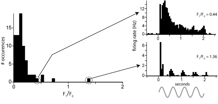
Figure 2.11. Distribution of simple and complex cells in the population of layer 2/3 Neurons………. 53 Figure 2.12. Stimulus-induced correlations do not affect measured synchrony……… 54
Figure 2.13. Network oscillations do not affect magnitude of correlated variability………….. 55
Figure 3.1. Optogentic inactivation of L6 corticothalmic cells………... 85
Figure 3.2. Effect of hyperpolarizing Ntsr1 cells on dLGN responses………. 86
Figure 3.3. Contrast dependence of Ntsr1 cell effects on dLGN units……….... 88
Figure 3.4. Effects of Ntsr1 cells across orientations, spatial frequencies and temporal frequencies……… 90 Figure 3.5. Effect of Ntsr1 hyperpolarization on dLGN spatial receptive fields………. 92
Figure 3.6. Effect of Ntsr1 hyperpolarization on dLGN temporal receptive fields………. 94
Figure 3.7. Effect of Ntr1 hyperpolarization on temporal precision of response to spatially uniform flicker……… 95 Figure 3.8. Effects of Ntsr1 hyperpolarization of dLGN pairwise coordinated activity……….. 96
Figure 3.9. No stimulus dependence of Ntsr1 effects on coordinated activity………... 97
Figure 3.10. Effect of stimulating Ntsr1 cells on dLGN visual responses………... 99
Figure 3.11. No change in dLGN burst statistics due to Ntsr1 hyperpolarization……….. 100
Figure 4.1. Optic chiasm stimulation generates compound field responses in mouse dLGN. 119 Figure 4.2. Spike activity in mouse dLGN following optic chiasm stimulation……… 120
Figure 4.3. Examples of linear and non-linear spatial summation in mouse dLGN………….. 121
Figure 4.4. Linearity of spatial summation in mouse dLGN……….. 123
Figure 4.5. Tuning characteristics of linear and non-linear units in mouse dLGN………. 124
Figure 4.6. Receptive field properties of single units in mouse dLGN……… 126
1
CHAPTER 1: INTRODUCTION
In the following work, we utilize the emerging model system of mouse vision to address several questions relating to output neurons from primary visual cortex (V1): layer 2/3 cortico-cortical neurons and corticogeniculate layer 6 cells. First, we address the independence of individual unit responses in layer 2/3 and the relationship to the underlying structure by measuring pairwise correlation on multiple time scales. We assess the functional role of a cell class in layer 6, the corticogeniculate population, and what effect these cells might have on the thalamus and V1 during visual responses. Below, we explain our motivation for exploring these questions, and why we chose to do so using the mouse early visual system.
Cortical structure and function
The cerebral cortex is widely held as the seat of cognition, from simple sensory (Hubel and Wiesel, 1968) and motor (Chouinard, 2006) processing, to complex decision-making (Heekeren et al., 2008) and executive activity (Kimberg and Farah, 1993; Brown and Bowman, 2002; Alvarez and Emory, 2006). Interest in the structure and function of the cerebral cortex dates to the birth of modern neuroscience (Ramon y Cajal, 1890; Penfield and Jasper, 1954). Recognition of the cortex as cognitive center predates this, at least to Thomas Willis in 1664, possibly to Erisistratus c.a. 260 BCE (Gross, 1999)
The painstaking work of early anatomists led to the description of a regular, repeatable organization across broad cortical areas, a layered structure with six, or eight (Ramon y Cajal, 1890), described layers. Contemporary consensus is a cortex with six primary layers
cortico-2
cortical neurons as well as subcortical projection neurons (Briggs, 2010; Thomson, 2010), with subcortical targets different than those of layer 5. These layer 6 neurons are of particular interest in this thesis, and are discussed in more detail below.
Although the structure varies slightly across cortical areas (Herculano-Houzel et al., 2008; 2013), it is remarkably similar across humans, other primates, and all mammals. A canonical operation across many cortical areas has been the target of speculation (Mountcastle, 1997; Douglas and Martin, 2007), though this has not yet been thoroughly demonstrated.
Primary visual cortex
3
‘simple cells’. Simple cells have separable, elongated receptive field subregions that match their orientation selectivity. A second selective convergence from layer 4 to layer 2/3, of cells with matching orientation preference but non-matching phase, may generate the phase-invariant orientation tuning in layer 2/3 (Alonso and Martinez, 1998). These phase-invariant cells are still orientation selective, but do display separable subregions and are called ‘complex’ cells.
This difference in phase sensitivity between layers 4 and 2/3 is also an example of the structure, or organization, of single cell response properties in primary visual cortex. In this case, the response property of phase sensitivity is organized across layers, with a systematic change from phase sensitive simple cells in layer 4 to the complex cells of layer 2/3, with layer 5
resembling the phase insensitivity in 2/3 and layer 6 a mix of simple and complex cells (Martinez et al., 2005; Hirsch and Martinez, 2006). Here the response properties change systematically through the depth. In most species, response properties are also organized across the dimension orthogonal to the depth: visual space, orientation preference, and ocular dominance all vary systematically across the cortical surface. Exceptions to this organization exist, like the lack of organization in orientation preference in mouse V1, a feature we explore in Chapter 2.
4
Correlated activity, pairs, and populations
For much of modern neuroscience, recording techniques have limited the experimenter to either recording from one isolated cell (like with single high impedance electrodes or intracellular recording with glass pipettes), or to the aggregate activity of an unknown, often uncontrollable number of cells (like with field potentials or fMRI). Both of these approaches have been fruitful, and promise to continue to be, especially as they are advanced (Long et al., 2011) and become better understood (Buzsáki et al., 2012; Einevoll et al., 2013). In this work, we have taken advantage of multi-tetrode recording to record the simultaneous activity of small populations of isolated single units, and analyze the correlation between these units at various timescales using various established techniques (Perkel et al., 1967a; Zohary et al., 1994), focusing on pairwise correlations. Correlations can and do occur beyond pairs of neurons (Schnitzer and Meister, 2003; Shlens et al., 2006); the frequency of these types of correlations in the early visual system is not yet clear, nor are any functional consequences.
What can be gained from considering pairwise correlated activity? The interpretation of pairwise correlations depends heavily on the stimulus conditions and the timescale of correlation measured. In the case of stimulus-corrected pairwise cross-correlograms (CCGs) on the scale of milliseconds (Perkel et al., 1967b; Gerstein et al., 1985), correlations can reflect the functional connectivity within the network (Aertsen and Gerstein, 1985; Ostojic et al., 2009). When both cells in a pair of neurons receive common excitatory input, these cells display a sharp CCG peak that straddles the zero line. Monosynaptic excitatory connections generate their own signature, a sharp peak offset from zero by approximately the synaptic latency (~2 milliseconds). Inferring functional connectivity from this form of correlation is useful for comparing said functional connectivity to other physiological measurements, usually other single cell physiological measurements.
5
readout neurons. In some cases, this type of correlated activity might carry additional stimulus information (Bohte, 2004), including the visual system (Dan et al., 1998; Shlens et al., 2006). While synchronous activity could be used to encode information, it is not clear if this approach is actually used in any neural system, a possibility explored in more detail in the Discussion.
Pairs of neurons can be correlated on other timescales, like correlated fluctuations in spike count over the period of a stimulus presentation, often seconds long. When these correlated fluctuations are a result of changing stimulus parameters they are called ‘signal correlations’. When these fluctuations are independent of stimulus parameters, they are termed ‘noise correlations’. Under some decoding regimes, noise correlations can reduce the
effectiveness of pooling (Zohary et al., 1994) and reduce the amount of stimulus information in the response (Abbott and Dayan, 1999; Nirenberg and Latham, 2003). The most commonly assumed neural readout regimes, like pooling models (Tolhurst et al., 1983) and variants of this (e.g., Law and Gold, 2009), are sensitive to this form of correlation. Because of the prevalence of these models, noise correlations have been the most extensively considered and measured form of pairwise correlation (Tolhurst et al., 1983; Kruger and Aiple, 1988; Kohn and Smith, 2005; Smith and Kohn, 2008; Cohen and Kohn, 2011).
The effect of correlations of any timescale on decoding of neural information depends on the identity and connectivity of correlated cells (Panzeri et al., 2003). It is therefore important to measure the structure of correlations on all timescales, and understand the mechanisms that generate them. In primate V1, the structure of correlations, both fast synchrony and noise
correlations, follows the organization of somatic organization preference. On the short time scale, pairs of cells with similar orientation preferences are more likely to receive common input. This true also on the longer timescale: nearby pairs of cells, and pairs of cells with similar orientation preference, have higher noise correlation (Smith and Kohn, 2008). It is not clear if this
6
absence of this orientation pinwheel organization in mouse visual cortex. We discuss the structure of mouse visual cortex below, and the results of our measurement of correlation in mouse V1 are presented in Chapter 2.
Mouse as a tool for visual cortical neuroscience
The mouse, while not a traditional model system used to study vision, is a useful system for investigating these questions for several reasons. First and foremost, the gross organization of the cortex resembles that of humans, as noted by Ramon y Cajal (in Pasik and Pasik, 2002). But the primary reason is the ready availability of transgenic tools that allow access to specific cell types. Several groups have embarked on large-scale generation of transgenic mouse lines, like the GENSAT project’s collection of GFP- or Cre recombinase-expressing lines (Gong et al., 2003; 2007) and the Allen Institute for Brain Science’s Cre-dependent tool mouse lines (Madisen et al., 2012). GFP-expressing lines offer the ability to visualize specific populations of cells for targeted recordings, for example PV+ interneurons (Sohya et al., 2007). Cre recombinase lines restrict the expression of this enzyme to a subset of cells. When combined with Cre-dependent transgene expression, either through viral introduction (Atasoy et al., 2008; Cardin et al., 2010b) or crossing with another transgenic line (Madisen et al., 2009; 2012), genetically encoded tools like algal and bacterial opsins (Bernstein and Boyden, 2011; Fenno et al., 2011), Ca2+ indicators (Zhao et al., 2011), or voltage indicators (Jin et al., 2012) are only expressed in that subset of Cre-expressign cells. This type of cell type specificity in vivo is not yet possible in other model systems.
The size and structure of the mouse brain also provides the opportunity for more complete sampling, relative to other model systems. Mice are lissencephalic, with a smooth cortical surface that lacks gyri or sulci. Because of this flat cortex, all cortical areas are accessible from a cranial window and vertical penetrations are possible in all areas. With the layered
7
imaging can be obtained with microprisms (Chia and Levene, 2009). The small size is also an advantage in the rostral-caudal and medial-lateral planes. Because the total cortical volume is small ( ~1.8 cm2, (Badea et al., 2007)), and the 25% of the cortex related to visual processing is even more manageable (~3mm by 3mm), simultaneous imaging and recording across visual areas is feasible (Glickfeld et al., 2013). The ganglion cell population of the mouse retina is better understood than any other species (Masland, 2012; Siegert et al., 2012), opening the possibility of understanding the inputs to central visual areas, and how those inputs might be transformed. Finally, mammalian high-throughput behavior is only possible with rodents (Meier et al., 2011; Scott et al., 2013), and our ability to exploit behavioral repertoire of mice is growing (Carandini and Churchland, 2013). The mouse as a model system for vision is not without downsides (Movshon, 2013), both experimental (e.g., small size) and biological (see below, e.g., poor spatial resolution and lack of directed eye movements), but other advantages make it a viable model.
What is known about mouse dLGN and V1 has grown rapidly in the last several years. Mouse retina has previously been the subject of intense characterization (Sun et al., 2002; Wässle et al. 2009; reviewed in Masland, 2012). The retinal outputs have been fully classified (Masland, 2012), and through combinatorial genetics individual ganglion cell classes can be isolated (Siegert et al., 2012). Much less is known about subsequent visual processing in mice. Anatomical evidence shows a lack of structure in mouse dLGN, but strikingly similar single cell morphology to other species (Krahe et al., 2011). In vitro work has shown the synaptic structure of mouse dLGN recapitulates that of cats. More specifically, the mouse dLGN has a triadic synaptic structure at retinal inputs, where the retinal bouton, the relay dendrite, and a
Acuna-8
Goycolea et al., 2008; Wijesinghe et al., 2013), even in the absence of information about the responses of mouse dLGN to visual stimulation.
Pioneering physiological work by Drager (1975), established that mouse primary visual cortex shares some canonical features of the better-described feline and primate visual systems: retinotopy, orientation selectivity, and simple and complex receptive fields. Behavioral
assessments showed mice to be capable of using visual information (Prusky et al., 2000). But because visual projections to superior colliculus had received the most attention (Drager and Hubel, 1975; Dunlop et al., 1996; Drescher et al., 1997), the neural basis of this behavior was questioned. Importantly, ablation of V1 revealed that this behavior was cortically mediated (Prusky and Douglas, 2004). Few other studies investigated canonical thalamocortical vision in mice.
The emergence of transgenic tools rekindled interest in mouse visual response properties. From this more recent wave, a new consensus has formed: poor spatial resolution, lack of orientation pinwheels, but good orientation tuning, temporal properties, receptive field structure, layer-like organization and parallel cortical processing streams (Gao et al., 2010). Measurement of receptive fields in the dLGN (Grubb and Thompson, 2003; 2004; Piscopo et al., 2013) and visual cortex (Niell and Stryker, 2008; Gao et al., 2010) have yielded V1 receptive fields about one order of magnitude larger than that seen in cats and primates, in the range of 5-15º in diameter. This poor spatial resolution is confirmed by preferred spatial frequency of drifting gratings, at < 0.1 cycles/º. In spite of this, orientation tuning can be very sharp in mouse V1 (Niell and Stryker, 2008; Gao et al., 2010; Zariwala et al., 2010). Mouse V1 has simple and complex receptive fields, with more simple receptive fields in the middle layers, corresponding a thalamorecipient layer. Like other species, response properties in V1 indicate parallel but separate processing streams (Gao et al., 2010).
9
organization of orientation selectivity that resembles several pinwheels, visible at macrocellular (Bartfeld and Grinvald, 1992) and single cell (Ohki et al., 2006) resolution. This orientation map is superimposed onto other maps, like the retinotopic map. Mice have a retinotopic map, but lack any somatic organization in orientation, a feature we exploit in our studies of the structure of correlation in mouse layer 2/3.
The usefulness of comparative biology in visual neurophysiology
Visual neurophysiology as a field has been dominated by work in cats and non-human primates, in cats because of the excellent spatial resolution, front-facing eyes, and availability of experimental animals, and in non-human primates because of the homology to human primates. Mice share a more recent common ancestor to primates (in the Euarchontoglires clade) than cats and primates (in the Boreoeutheria magnorder) (Kriegs et al., 2006). Homologies in visual system organization between mice and primates represent traits either preserved from the common cat-primate ancestor or that arose before the divergence of cat-primates and mice. Any of these homologies represent a fundamental feature of visual system organization preserved across evolutionary time. The visual receptive field first described in the invertebrate limulus (Ratliff and Hartline, 1959) bears a great resemblance to retinal and dLGN receptive field, and this homology across evolutionary distance cemented the receptive fields as a basic concept in visual system organization. This is an example of how the comparative approach, performing measurements of known quantities in one system in a new species can reveal factors important to basic function and preserved across species. We take this approach in making measurements of pairwise correlation structure in mouse layer 2/3 (Chapter 2) and dLGN response properties known in cats and monkeys in mice (Chapter 5).
Optogenetics
10
mammalian cells using expression of bacterial or algal opsins and exogenously applied light is a rapidly spreading technique. It offers some significant advantages over other methods for manipulating neural activity: the opsins are genetically encoded, allowing for cell-type specific expression due to viral tropism (Nathanson et al., 2009), or other combinatorial expression systems such as the FLEX system (Atasoy et al., 2008). These opsins allow for single millisecond precision in spike generation, and can achieve similar timescale hyperpolarization (Chow et al., 2010). Continuing engineering of these proteins has improved the temporal resolution, increased sensitivity to allow for transcranial stimulation (JAWS, Boyden laboratory, MIT), and generated new tools like step-function opsins (Diester et al., 2011). In the early use of these tools, much focus has been on activating cells, perhaps due to the historical difficulty in achieving specific stimulation. Here, we utlize Channelrhodpsin-2 (ChR2) to stimulate a specific cell type, but in support of more extensive loss of function experiments using Archaerhodopsin-3 (Arch) to hyperpolarize during visual stimulation.
These opsins can be powerful tools for understanding the function of cell types in both physiology (Cardin et al., 2009; Adesnik et al., 2012), behavior (Gerits et al., 2012; Jazayeri et al., 2012), and disease (Gradinaru et al., 2009; Kravitz et al., 2010) through loss-of-function
experiments, and for elucidating mechanisms of cell type action through gain-of-function activation in specific and varied experimental contexts.
The function of corticogeniculate-projecting cells
Anatomical tracings by Ramon y Cajal led him to comment on the number and density of fibers from cortex to thalamus, saying of them “An infinite number of fibers, coursing together with the previous ones, enter the [thalamic] nucleus under study and generate a fine and dense plexus” (in Pasik and Pasik, 2002). Indeed later anatomical studies led to the oft-quoted estimate of corticothalamic fibers outnumbering thalamocortical fibers by and order of magnitude
11
the deeper layers of V1, in both layers 5 and 6. However, the corticothalamic fibers of layer 5 do no project to primary sensory nuclei like the dLGN, but rather to secondary thalamic nuclei like pulvinar (Jones 2007). Corticothalamic axons originating in layer 6 project to both primary and secondary nuclei (Briggs, 2010; Thomson, 2010; Tombol,1984). Here, we focus on the corticothalamic axons in layer 6 projecting from primary sensory cortex to primary sensory thalamic nuclei, and will refer to these axons as ‘corticogeniculate’.
Corticogeniculate (CG) axons follow the optic radiation back from cortex to dLGN, leave an axon collateral in the perigeniculate or reticular nucleus, and continue into dLGN to form synapses directly onto relay cells and interneurons. The synapses of CG axons onto relay cells are found at distal dendritic areas; CG axons excite relay cells via type 1 metabotropic glutamate receptors (mGluR1s) (McCormick and Krosigk, 1992; Rivadulla et al., 2002) and contain an NMDA component (Scharfman et al., 1990) at synapses that depress strongly during repeated stimulation (Jurgens et al., 2012). In addition, these axons bifurcate before exiting V1, sending an axon collateral up to layer 4. This local cortical projection targets all cell types in layer 4, including the excitatory stellate cells and local interneurons. Electron microscopy suggests a slight bias toward inhibitory cells in layer 4 (McGuire et al., 1984) and a net inhibitory effect. This net inhibition is supported by recordings in dLGN following stimulation of cortex (Widen and Amjone Marsan 1960; Olsen et al., 2012).
12
conditions (Kalil and Chase, 1970; Kayama et al., 1984; Molotchnikoff et al., 1986; McClurkin et al., 1991).
While most of these studies used drifting sinusoidal gratings (McClurkin et al., 1991; Przybyszewski et al., 2000; Rivadulla et al., 2002; Andolina et al., 2007), others used bars (Vastola, 1967; Hull, 1968; Kalil and Chase, 1970), and the size of stimuli ranged across studies. As a result, these spatial disparities have been invoked to explain the disparities in results: misaligned RFs providing suppression and aligned RFs facilitation. Direct evidence supporting this hypothesis has been obtained with paired recordings of single CG axons and single dLGN cells (Tsumoto et al., 1978). Further evidence comes from the effect of cortical activity on elements of dLGN single unit non-classical RFs. (Murphy and Sillito, 1987, 1988; Murphy et al., 1999; see Sillito and Jones, 2002). Another approach has been to focus on the temporal structure of dLGN responses and how CT projections alter this structure (Funke et al., 1996; Worgotter et al., 1998). Some consensus about CT feedback has emerged: a weak modulatory effect, not affecting spatiotemporal properties, that has divergent effects through depolarization to change firing mode. Even so, papers continue to appear that challenge this model (Andolina et al., 2013).
Here, we use the GN220 Nstr1-Cre line, created and distributed by the GENSAT project (Gong et al., 2007) to characterize specific and general effects of a genetically specified
13
from previous approaches in specificity and in species, we attempted to use the simplest stimuli possible and to comprehensively characterize the effect of Ntsr1-CG cells. Briefly, we find similar results to some of those reported previously: both facilitative and suppressive effects of Ntsr1-CG projections that do not alter spatiotemporal properties, though we do not see evidence for
14
CHAPTER 2: THE STRUCTURE OF PAIRWISE CORRELATION IN MOUSE
PRIMARY VISUAL CORTEX REVEALS FUNCTIONAL ORGANIZATION IN THE
15
Abstract
16
Introduction
Throughout sensory systems, neurons are organized by response preference, so that like-responding neurons are close to each other, creating a functional map [e.g., orientation pin- wheels in primary visual cortex (V1)]. Despite the ubiquity of maps, their role is unclear. For example, although rodent V1 lacks an orientation map (Ohki et al., 2005), single-cell orientation selectivity is not grossly different than in species with an orientation architecture (Niell and Stryker, 2008; Gao et al., 2010). In addition, correlations of spike output within a population of responding neurons are also organized by the underlying functional architecture. In V1, pairwise correlated activity depends on the pair’s relative orientation preference (Kohn and Smith, 2005; Smith and Kohn, 2008), relative distance (Kruger and Aiple, 1988; Gawne and Richmond, 1991; Smith and Kohn, 2008), and among distant cells it is only observed between cells with similar orientation preference (Ts'o et al., 1986).
Correlations reflect the functional connectivity within a network (Perkel et al., 1967a). In addition, correlations can affect representation of information by a network in diverse ways, including influencing pooling (Zohary et al., 1994; Abbott and Dayan, 1999; Romo et al., 2003) and enhancing post- synaptic integration (Alonso et al., 1996; Cardin et al., 2010a). Any role for these correlations in sensory coding depends on the magnitude of correlation and the structure of correlation relative to space and stimulus parameters (Abbott and Dayan, 1999; Deneve et al., 1999; Pouget et al., 1999). In the presence of an orientation map, nearby neighbors often share selectivity for space and orientation, making the local structure of pairwise correlation difficult to determine.
17
Callaway, 2005) and within (Ko et al., 2012) layer 2/3 networks would result in a structure of pairwise correlations between neurons that is dependent on orientation and distance even in the absence of functional architecture.
We measured pairwise correlation on two timescales: a longer timescale of mean spike count on a trial-to-trial basis (rsc) and a short timescale of synchrony within tens of milliseconds.
We found that pairwise synchrony is dependent on the distance and the difference in orientation preference between the cells in each pair. Both visually evoked and spontaneous rsc are also
18
Materials and Methods
Animal Preparation and Surgery
All procedures were done within the guidelines of the National Institutes of Health and were approved by the University of Pennsylvania Institutional Animal Care and Use Committee. Adult C57/B6 mice (8– 24 weeks) were initially sedated with a mixture of xylazine (10 mg/kg) and fentanyl (10 µg/kg); anesthesia was induced with a high concentration of isoflurane (5%) and maintained with continuous inhaled isoflurane (0.1–1%). Additional doses of fentanyl (5µg/kg) were administered every approximately 2 h to maintain anesthetic plane. The depth of anesthesia was monitored by heart rate (maintained between 300 and 600 beats/min), pupil dilation, pinch reflex, and fol- lowing the opening of the craniotomy by the level of synchronous activity in the local field potential (LFP). After placement in a stereotactic apparatus, eye moisture was maintained by application of a transparent lubricant and body temperature was maintained at 37°C by rectal monitoring and a heating pad (FHC In c., Bowdoin, ME, USA). A 2-by-2 mm craniotomy was opened over V1. To minimize damage during electrode penetration, the dura was resected across the majority of the craniotomy using a dura hook and the exposed surface was coated with a layer of silicon oil. Following surgery, the entire stereotactic apparatus was rotated 60° to position the contralateral eye in front of t he display screen.
19
Electrophysiology
Following surgery, an array of four to six tetrodes (Thomas Recording GmbH, Giessen, Germany) arranged either linearly or concentrically was inserted into V1 perpendicularly relative to the cortical surface. In both configurations, the tip-to-tip space between neighboring tetrodes was 254
µm. Individual tetrodes were 100 µm in diameter with a central contact at the tip approximately 40
µm below three concentrically arranged contacts around the shaft approximately 20 µm from each other. Signals were preamplified by the tetrode drive and amplified, individually filtered, and acquired at 30 kHz using a Cheetah 32 acquisition system (Neuralynx, Boseman, MT, USA). High-frequency spiking activity was isolated at each contact by filtering between 600 and 6000 Hz. A single channel from each tetrode was duplicated and filtered 0.1–375 Hz to record an LFP. Each tetrode was individually inserted to an initial depth of 100–160 µm. Following a rest period of at least 30 min, each tetrode was lowered through the cortex in 2-µm steps until at least one strong unit was present; in this dataset, all tetrodes were stopped before reaching approximately 350 µm below the cortical surface, the putative boundary of layers 3 and 4.
Visual Stimuli
20
Stryker 2008; Gao et al. 2010; Niell and Stryker 2010). The 70° stimuli were sufficiently large, as the visual space recorded by our most distantly spaced electrodes is approximately 30°; given the median size of a mouse V1 receptive field (Gao et al., 2010) of all cell pairs recorded up to 500
µm are at least partially overlapping (Bonin et al., 2011).
Spike Clustering and Data Analysis
Spike waveforms from each tetrode were clustered into individual units offline using a mixture of algorithmic and manual sorting (Spike- Sort3D, Neuralynx). Waveforms were initially sorted using KlustaKwik and subsequently manually refined (e.g., Fig. 1A,B). All clusters with spikes in the 0– 1-ms bin of the interspike interval histogram were strictly rejected. To assess the quality of separation of the identified single units, we measured isolation distance and the L-ratio for each cluster (Fig. 1C), which indicate the distance of the center of the cluster from the noise and the quality of the moat around the cluster, respectively (Schmitzer-Torbert et al., 2005). An example set of clustered data in Figure 1A–C shows the isolation of 6 single units from one tetrode, with isolation distances >10 and L-ratios <0.4.
All analysis of single-cell and pairwise spikes was done using Igor Pro 6.0 (Wavemetrics, Lake Oswego, OR, USA) at 1-ms resolution. Orientation tuning was quantified using the average number of spikes over the duration of stimulus presentation. The orientation tuning curves, across the range 0–360°, were fit with the von Mises funct ion (Swindale, 1998):
21
between the maxima for a pair of cells. Orientation selectivity index (OSI) was calculated, from raw responses, as the difference between responses at preferred and orthogonal orientations as follows:
– !" !"
where Rpreferred is the response at the preferred orientation, as deter- mined by the circular Gaussian fit, and Rortho is the response at the orientation 90° from R preferred. All reported p-values were calculated using the Wilcoxon rank-sum test.
Correlation Measures
Correlation between pairs of cells was measured on two timescales: trial-to-trial variation in spike count (rsc) and synchrony within 10 ms. Correlated variability was defined as the shared
variation, either increase or decrease, in the number of spikes fired over a given time window. The time window used here was the duration of stimulus presentation, which was 2 s. To
calculate the rsc for a given pair, the response of each cell was assigned a z-score for each trial:
#
$%&where x is the rate on a given trial, µ the average rate for all trials, and σ the variance. The Pearson correlation was computed as the product of z-scores between a pair summed across all trials:
'
() *∑ ,-
*67 .&/ – .012 -
3/& – 30425
where n is the number of trials, Xi and Yi the rates for each cell on a given trial, X and Y the sample means for each cell, and σX and σY the sample variance for each cell.
22
correlation; to account for differences in firing across the population, each CCG was divided into the geometric mean of the firing rates of the pair of cells. CCGs were further corrected by the jitter-correction method (Smith and Kohn, 2008; Harrison and Geman, 2009)) using a 50-ms jitter window. Choosing this window size destroys all correlations <50 ms in the correction term, but preserves correlation on all longer timescales. Subtraction of this correction term isolates only the correlation in the raw CCG that occurs on the <50 ms timescale. The presence of a synchronous peak was assessed using a threshold set 2 standard deviations (SD) above the mean level of correlation. Mean correlation was here defined as the mean of the corrected CCG from 100 to 200 ms. The magnitude of synchrony was determined as the area between the threshold and the CCG ±10 ms from the zero line. The correction method used did not affect the presence or the size of synchronous peak (see Fig. 3C,D). All measurements reported here are based on jitter-corrected CCGs.
To statistically justify the separation of CCG shapes into classes, we measured several parameters from each CCG: width, peak lag, and symmetry. Width was measured at the crossing of the significance threshold. Peak lag was the difference between zero and the time at which the peak occurred. CCG symmetry was measured as follows:
89::;'9
<= <>?@23
Results
Our goal was to quantify visually driven and spontaneous pair- wise correlations of neurons in the supragranular layers 2 and 3 (L2/3) of mouse V1 as a function of their relative distance and their similarity of orientation preference. We recorded single neurons from L2/3 of V1 of anesthetized mice (n = 38) using six independently positioned tetrodes. To minimize sampling bias, the
position of the tetrodes in L2/3 was not readjusted once a set of cells was detected within the first 370 µm from the pial surface. Individual units were identified using an offline, partially automated clustering procedure (see Materials and Methods; Fig. 1A–C). Each tetrode sampled up to seven single neurons simultaneously. To maximally drive spiking activity from each population of simultaneously recorded neurons, we used full screen, 100% contrast, drifting sinusoidal gratings optimized in spatial and temporal frequencies for mouse V1 (0.06 cycles/°, 2Hz; Niell and Stryker 2008; Gao et al. 2010). The example cell in Figure 1D responded to repeated presentations of an optimally oriented drifting grating with a nonmodulated increase in the firing rate (mean = 7.2 Hz). The visual response was robust and consistent across trials, as shown by the raster plot
24
orientation (>0.8 OSI) and a large number with weak selectivity (<0.4 OSI). However, there were only 3 untuned cells in our database with OSIs <0.2 (Fig. 1F, left panel). The response properties of the cells in our database were consistent with recent quantitative descriptions of mouse V1 (Niell and Stryker 2008; Gao et al. 2010).
Quantification of Correlation
We quantified correlated firing for each pair of simultaneously recorded cells on two timescales, according to previously established methods (Perkel et al. 1967; Smith and Kohn 2008): (1) synchrony, which measures the pairwise correlation of spike times within ±10 ms, and (2) correlated variability (also called noise correlation, or rsc), which measures the trial-to-trial correlation of spike counts over the duration of each trial (2 s). All measurements of correlation were made from responses to 2 Hz drifting gratings of varying orientation, sufficient to elicit a response from many cells on each trial. Correlations induced by the temporal frequency of these stimuli are broader than the synchrony measured.
We quantified synchrony from the pairwise CCGs (bin = 1 ms) normalized by the
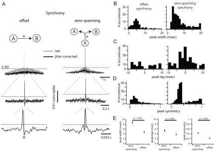
geometric mean firing rate and corrected using the subtraction of a 50-ms jitter-correction term to remove stimulus-induced correlation (see Materials and Methods). The “magnitude” of synchrony was the area of the central peak (±10 ms) of the CCG exceeding 2SD above base- line noise (Fig. 2A, the dotted line indicates 2SD; see Materials and Methods). The “probability” of
synchrony was the ratio of the number of pairs with a significant peak over all recorded pairs. We further subdivided the population of significant CCGs based on the position of the peak with respect to the zero line. A positive peak entirely displaced from the zero line was classified as “offset” synchrony (Fig. 2A, left; n = 90/4160).
25
explanation for such a shape (Perkel et al. 1967; T’so et al. 1986; Ostojic et al. 2009). A positive peak straddling the zero line was classified as “zero spanning,” and is consistent with a shared source of excitatory input (Fig. 2A, right; n = 234/4160; Perkel et al. 1967). Most zero-spanning peaks were not centered over the zero line (164/234 zero-spanning peaks). The remainder of zero-spanning peaks were centered on zero (70/234). This ad hoc classification of CCGs as offset or zero spanning was supported by the difference in the distribution of peak widths (Fig. 2B), showing statistically different means (Fig. 2E; P < 0.005). The distribution of peak lags, defined as the time of peak relative to zero, was complementary: zero-spanning CCGs were centered on zero (Fig. 2C, right), while offset CCGs had a bimodal distribution with centers at 5 and −5 ms (Fig. 2C, left). The absolute peak lag was significantly larger for offset CCGs than zero-spanning CCGs (Fig. 2E, center; P < 0.005). To formalize the difference between the two CCG classes, we measured peak symmetry relative to zero (see Materials and Methods). This value is 1 for peaks exactly centered on the zero line and 0 for peaks fully shifted from the zero line. All offset CCGs showed high asymmetry (Fig. 2D, left). Zero-spanning CCGs (Fig. 2D, right) had a bimodal distribution of symmetries, with a population of highly symmetrical CCGs
(symmetry >0.4; mean: 0.79 ± 0.02) and a population of asymmetrical, yet zero-spanning, CCGs (symmetry <0.4; mean: 0.26 ± 0.005). The subset of symmetrical zero-spanning CCGs was similar to the full population of zero-spanning CCGs in all measurements made subsequently (Supplementary Fig. 2), and so all zero-spanning CCGs were grouped to maximize statistical power.
26
3C,D). The removal of this onset transient reduced the peak of some pairs slightly (Fig. 3D), but the reduction in CCG magnitude was not significant and smaller than the percentage of spikes removed.
We included pairs recorded on the same tetrode, despite the inability to detect near synchronous spikes for such pairs due to acquisition enforced dead times; because of this, we removed the zero-lag bin from all CCGs from pairs on the same electrode. Peaks from the cells recorded on the same tetrode reflected both forms of synchrony (e.g., Fig. 4A). Removing the zero-lag bin affected the classification of CCGs as offset or zero spanning in only 1 of 90 offset CCGs.
We quantified trial-to-trial correlated variability, or rsc, as the Pearson correlation coefficient of standardized mean firing rates across the duration of a trial. This measure is equal to 1 when the covariance between a pair is perfect and 0 when a pair of cells does not covary.
Synchrony as a Function of Orientation Preference
27
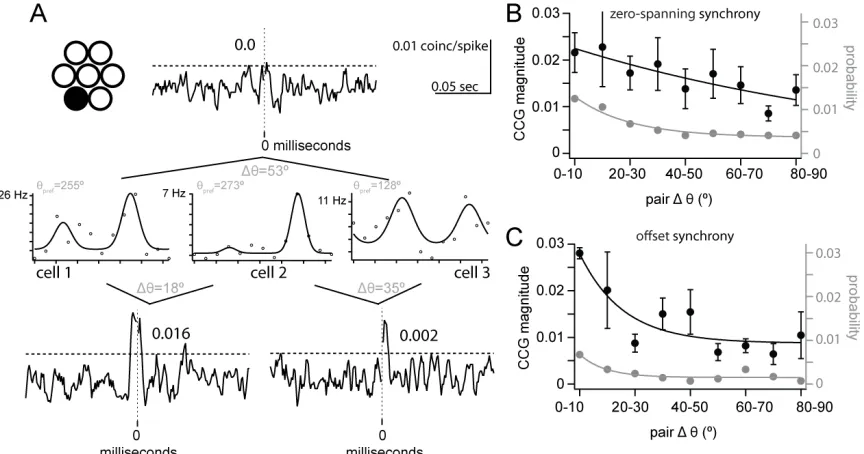
with a magnitude that was dependent on the similarity of orientation preference despite the proximity of the neurons. The strongest synchrony was observed within the pair with the most similar orientation preference (CCG peak = 0.016, cells 1 and 2), while the pair with largest difference in orientation preference showed no significant synchrony (cells 1 and 3), and the intermediate orientation preference difference showed weaker synchrony (CCG peak = 0.002, cells 2 and 3). This example is inconsistent with the synchrony observed between neighboring neurons at pinwheel singularities in cat visual cortex, where the magnitude of synchrony of nearby neighbors is unaffected by difference in orientation preference (Das and Gilbert, 1999).
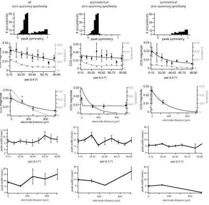
We obtained population measures of the relationship between synchrony and orientation tuning separately for zero-spanning (Fig. 4B) and offset CCGs (Fig. 4C). For zero-spanning synchrony, the probability (gray) and magnitude (black) of synchrony were dependent on ∆θ and were fit by exponential decay functions (x2prob 1⁄4 4 10_4; x2mag 1⁄4 4 10_5; Fig. 4B). The probability of zero-spanning synchrony was higher for cell pairs whose preferred orientations differed by <30° than for cell pairs with less similar orientation tuning (Fig. 4B). As a function of ∆θ, the magnitude of zero-spanning synchrony decreased more slowly (τmag = 126.2°) than the probability (τprob =
19.9°; Fig. 4B). To determine a criterion ∆θ value for magnitude zero-spanning synchrony, we compared each 10° ∆θ bin to the first bin (0°– 10°); the first signific antly different bin was 40–50° (P = 0.03), and all subsequent bins were significantly different (P < 0.05). We conclude that zero-spanning synchrony is both strongest and most likely within pairs with ∆θ < 40°, reflecting the specificity of L4 projections to L2/3.
For offset synchrony, probability and magnitude were also dependent on ∆θ and were fit by exponential decay functions (x2prob 1⁄4 7:5 10_5 ; x2mag 1⁄4 8:8 10_5 ; Fig. 4C). The magnitude of offset synchrony decayed similar to probability (τmag = 15.6° and τprob = 9.3°). The probability
of offset synchrony was small and relatively flat for ∆θ greater than 30° (Fig. 4C). The criterion ∆θ
28
different (P < 0.05); the exponential decay saturated >40°. We conclude that the strength of offset synchrony is strongest within pairs with ∆θ < 40°, consistent with in vitro measurements of synaptic connections between neighboring cells of known orientation preference (Ko et al. 2011).
The dependence of synchrony on firing rate could affect this measurement (la Rocha et al., 2007), as dissimilarly tuned cells are less likely to fire spikes on the same trial. However, across ∆θ, rate-matched pairs yielded exponential fits similar to the full dataset (data not shown), indicating that the effect of stimulus selectivity on synchrony is not dependent on rate.
Synchrony as a Function of Distance
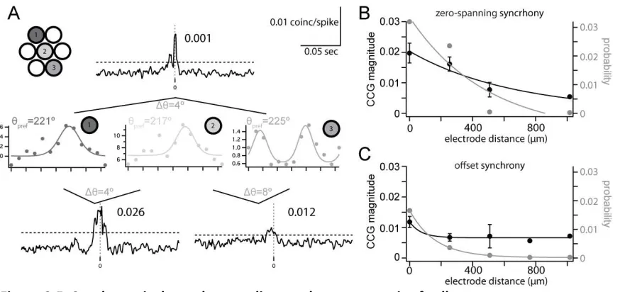
We next considered how the distance between a pair of cells affects synchrony independent of their difference in orientation preference. We found that the distance between a pair of cells, as measured by electrode spacing, significantly affected the probability and magnitude of both types of synchrony. The example in Figure 5A shows three neurons recorded from three tetrodes spanning 508 µm. The orientation preference of these cells was very similar, differing by only 4– 8° (cell 1: 221°, cell 2: 217°, and cell 3: 225°). Despite the considerable distance between cells 1 and 3, they had a significant zero-spanning CCG peak (magnitude = 0.012). One closer pair had a larger synchrony magnitude in spite of having similar ∆θ (cells 1 and 2: 0.026), demonstrating the effect of distance on the magnitude of zero-spanning synchrony, while another closely spaced pair had weaker synchrony (cells 2 and 3: 0.001).
29
(χ2 = 2.2 × 10⁻⁶; Fig. 5C) much faster (τprob = 162.9 µm) than zero-spanning synchrony. The magnitude of offset synchrony decayed quickly (x2mag 1⁄4 5:4 10_6; τmag = 72.7 µm), though the few observations of offset synchrony at distances >508 µm were not significantly smaller than those at smaller distances (P > 0.05). Our measurements constrain the spatial extent of the functional networks described by spanning and offset synchrony. The spread of zero-spanning synchrony suggested a wider feedforward network, approximately 1 mm in diameter, compared with a more constrained functional network of offset synchrony, <400 µm in diameter.
Width of Synchrony as a Function of Distance and Orientation Preference
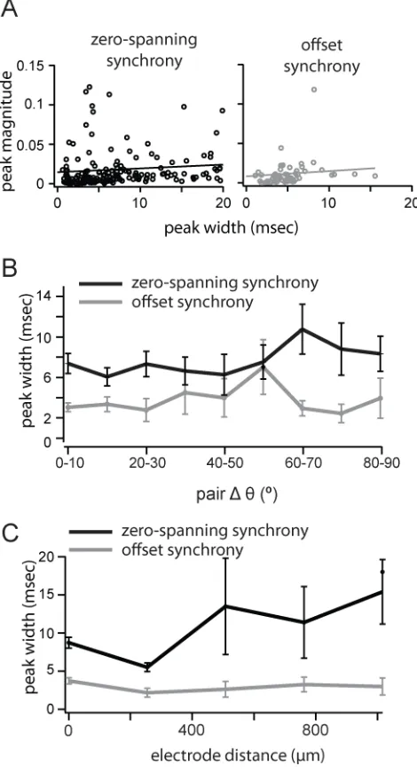
The width of the synchronous peak can affect the measurement of synchrony strength and may be regulated by distinct mechanisms in V1 (Kohn and Smith 2005). Within the allow- able window of ±10 ms, we measured the width of the synchronous peak at the point of crossing the 2SD significance threshold. Offset synchrony peaks were significantly narrower (4.8 ± 2.77 ms) than zero-spanning synchrony (8.7 ± 3.29 ms; P < 0.005, Wilcoxon rank test, Fig. 2B). Narrower offset synchrony peaks are compatible with the underlying hypothesis that this form of synchrony arises from a single source, while zero-spanning peaks can arise from multiple sources. For both types of synchrony peak, peak width was positively correlated with CCG magnitude, though weakly (Fig. 6A; slope of the linear fit, zero-spanning: 0.48 × 10⁻³ ± 0.28 × 10⁻³; offset: 0.67 × 10⁻³ ± 0.45 × 10⁻³). There was no trend in peak width, either offset or zero-spanning, over difference in preferred orientation (Fig. 6B). Zero-spanning synchrony was narrower for nearby cells (<500
30
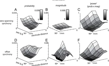
Synchrony as a Function of Both Orientation Preference and Distance
Finally, we measured the codependence of both forms of synchrony on distance and ∆θ, a measurement that is straightforward here because distance and orientation preference are independent across the topography of mouse visual cortex (i. e., there are no orientation
pinwheels). Across a network of approximately 1 mm, zero-spanning synchrony is more likely and of larger amplitude for neurons with similar orientation preference (Fig. 7A–C). The probability and magnitude of zero-spanning synchrony decreased as a function of distance across all ∆θ. Notably, probability and magnitude appeared to have the same structure over distance and ∆θ, reflecting the stimulus specificity of the common input presumably originating in L4 and
responsible for the orientation selectivity of L2/3 neurons.
In contrast, the probability of offset synchrony was nearly independent of ∆θ for nearby cells (<500µm; Fig. 7D). However, the magnitude of offset synchrony between neighbors was highly dependent on ∆θ, falling for ∆θ > 20°. Thus, within smaller networks (<500µm),
connectivity is wide- spread but the strength of connectivity is ∆θ specific. For further separated pairs (>500 µm), the probability of connection was lower and limited to pairs with ∆θ < 30°; observations of offset synchronous pairs separated by >500 µm and with ∆θ > 30° were rare and always of very small magnitude (Fig. 7E). Thus, our measurements show that the mechanisms that generate zero-spanning, but not offset, synchrony between nearby cells (within
approximately 200 µm) show specificity to the orientation preference within the pair. For longer-range connections, both forms of synchrony show specificity for the orientation preference within the pair.
31
parametric dependence on distance and ∆θ as probability and magnitude alone. That is, the strongest zero-spanning power was for nearby and similarly tuned cells, decreasing with both distance and ∆θ (Fig. 7C).
The power of offset synchrony had a similar parametric dependence as the power of zero-spanning synchrony, again showing the strongest functional connectivity for nearby and similarly tuned cells, decreasing with both distance and ∆θ (Fig. 7F). Unlike zero-spanning power, the structure of the power of offset synchrony was however created by the combination of
complementary dependencies: the effect of ∆θ at distances >500 µm was conferred by the probability (Fig. 7D), while the effect of ∆θ at local distances was conferred by the magnitude (Fig. 7E). These plots demonstrate that functional connectivity can be organized in the absence of a functional architecture. In addition, the powers of functional connectivity of zero-spanning and offset synchrony show matching organization: highest for nearby cells with the similar orientation preference, lowest for distant pairs of the orthogonal orientation preference. Our data show functional connectivity that reflects the synaptic specificity of input to and within layer 2/3, in agreement with predictions based on in vitro measurements (Yoshimura et al., 2005; Ko et al., 2012).
Correlated Variability
32
Reich et al. 2001; Kohn and Smith 2005; Smith and Kohn 2008) and cat V1 (Das and Gilbert, 1999). We quantified a “spontaneous” rsc using the periods between presentations of visual stimuli. To account for adaptation effects from the preceding stimulus, we calculated a
spontaneous rsc from periods subsequent to stimuli of the same orientation, and averaged across all orientations. Ac- counting for adaptation effects reduced spontaneous rsc primarily for nearby pairs (data not shown). The rsc calculated from epochs of spontaneous activity (0.15 ± 0.005; Fig. 8A, black histogram, mean indicated by black arrow) was not significantly higher than evoked rsc (P = 0.13). Spontaneous rsc was highly correlated with evoked rsc (linear fit slope = 0.82 ± 0.02, R2 = 0.47, Fig. 8A, right).
Correlated Variability as a Function of Distance and Orientation Preference
At our spatial scale, we observed a dependence of evoked rsc on distance, well fit by an exponential decay function (χ2 = 0.004, τ = 209.9 µm; Fig. 8B, left panel). It is important to note that although the area of cortex over which we measured correlation (approximately 1mm) is more limited than in studies of other species, the span of visual space covered by our recordings is actually slightly larger (approximately 60° of v isual space; Kalatsky and Stryker 2003). The decay in evoked rsc with distance (τ = 209.9 µm; Fig. 8B, left) was most similar to the decay in offset magnitude (τ = 162.9 µm; Fig. 5C). The fit parameters used to fit the magnitude of offset synchrony fit the decay of evoked rsc with χ2 = 3 × 10⁻⁴, consistent with a conclusion that trial-to-trial correlated variability is at least partially mediated by connectivity within L2/3.
We further investigated correlated variability by examining the relationship between ∆θ
33
increasing ∆θ, evoked rsc in- creased at larger ∆θ leading to a slightly U-shaped dependence (Fig. 8C, left). Still, this dependence was fit with an exponential decay (τ = 11.7°, χ2 = 2 × 10⁻⁴).
Finally, we were able to measure the codependence of evoked rsc on distance and ∆θ
(Fig. 8D, left), as we did for synchrony (Fig. 7). At short distances, evoked rsc depended on ∆θ, while at distances >500 µm, rsc was independent of ∆θ. The two-dimensional relationship of evoked rsc closely matched that of synchrony power. We further explore the relationship between evoked rsc and functional connectivity below (Fig. 10). The structure of evoked rsc demonstrates that correlation can be organized in the absence of functional architecture.
Correlated Variability of Spontaneous Activity
The correlated variability of spontaneous activity could have different spatial properties than that of evoked activity. Similar to evoked rsc,, we observed a dependence of spontaneous rsc on the distance between the pair (Ch'ng, 2010) (τ = 235.3 µm, χ2 = 0.013; Fig. 8B, right). ∆θ had a weak effect on the measured spontaneous rsc (τ = 3.0°, χ2 = 3 × 10⁻⁴; Fig. 8C, right). A stronger dependence of spontaneous rsc on ∆θ was apparent for nearby pairs (Fig. 8D, right), as has been previously observed in rodents (Ch’ng and Reid 2010). The relatively flat spatial and orientation tuning structure of spontaneous rsc (Fig. 8D, right) suggests that the source of input responsible for these correlations operates nonspecifically over a distance >1 mm in mouse V1, distinct from the sources of synchrony.
Correlated Variability as a Function of Network State
34
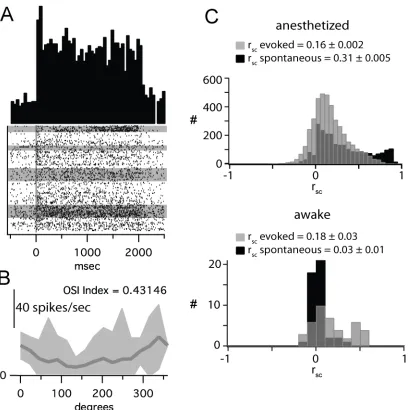
observed here are not physiologically relevant (Ecker et al., 2010), namely that correlated variability is aberrantly increased by several factors, including clustering error and anesthetic-induced network state. To assess the role of network state on correlated variability, we quantified network synchronization using the spectral content of LFP recordings. The level of gamma activity either immediately preceding or during evoked activity did not affect the value of rsc observed (Supplementary Fig. 3). To more directly assess the role of anesthesia on rsc, we measured rsc in awake, head-fixed mice under the same visual stimulus paradigm. Under these conditions, spontaneous and evoked firing rates were higher than under anesthesia (spontaneous mean: 2.8 ± 2.12 Hz; evoked mean: 8.082 ± 7.52 Hz; Fig. 9A), but cells showed similar
orientation tuning (Fig. 9B). As such, these conditions eliminate two of the proposed confounding factors in measuring rsc: anesthetic-induced synchronization and dampened firing rates. Despite this, evoked rsc was very similar in the anesthetized and awake states (anesthetized: 0.16 ± 0.002, awake: 0.18 ± 0.03, P = 0.34; Fig. 9C). In contrast, spontaneous rsc (0.03 + 0.01) was much lower in the awake state than that observed in the anesthetized state (anesthetized: 0.36 ± 0.004, P < 0.01; Fig. 9C), likely due to the lack of a slow oscillation in the LFP. In summary, measurements of correlation in the awake state were not different than those measured under our anesthetic regime.
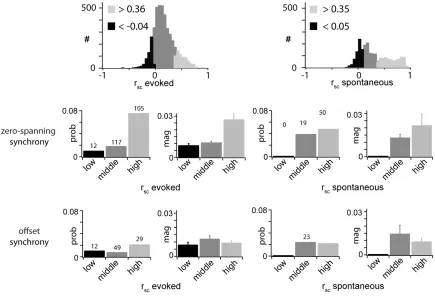
The Relationship Between Correlated Variability and Synchrony
35
of rsc values (Fig. 10A). The thresholds for high (evoked rsc > 0.36; spontaneous rsc > 0.31; Fig. 10A,B, light gray) and low (evoked rsc < −0.04; spontaneous rsc < −0.02; Fig. 10A,B, black) classes were set one SD above and below the mean, respectively. The probability (Fig. 10C, left) and magnitude (right) of zero-spanning synchrony within each rsc class were highest for pairs with high evoked rsc. In contrast, the probability and magnitude of zero-spanning synchrony were highest for pairs close to the mean value of spontaneous rsc (Fig. 10C, right), indicating a
36
Discussion
We measured the pairwise correlation of spike output in mouse V1 in response to visual stimulation on two timescales: synchronous spikes within ±10 ms and covariations in the mean evoked firing rate. Each has implications for information processing, depending on the neural implementation of de- coding. We measured synchrony using pairwise CCGs and found that both the magnitude and probability of positive CCGs were a function of the difference in orientation tuning and distance between the two neurons in the pair, a functional structure despite the absence of columns.
We measured pairwise correlated variability (rsc) of mean trial spike counts using Pearson’s correlation coefficient. We found a small but significant value of rsc (0.16 ± 0.01), similar to most of the studies in the literature. This magnitude was not due to anesthesia, as it was not significantly different in awake, actively moving mice. We found that rsc depended on inter- neuronal distance and on the difference of orientation preference. Our results revealed a structure of neuronal correlations independent of a functional architecture.
Synchrony and Functional Connectivity
37
(Thomson and Lamy 2007) or electron microscopy (Bock et al. 2011), we consider this evidence of a direct excitatory connection (Perkel et al. 1967; Ostojic et al. 2009).
At the short distances recorded by a single tetrode, the probability and magnitude of zero-spanning synchrony decreased as a function of relative orientation preference (∆θ) (Fig. 7). As in columnar organization, L2/3 visual responses were dominated by orientation-specific L4 input, in agreement with specific connectivity between L4 and subnetworks of L2/3 pyramidal cells demonstrated in rodent visual cortex in vitro (Yoshimura and Callaway 2005). In contrast, the probability of offset synchrony at short distances was not dependent on ∆θ, consistent with diffuse L2/3 pyramidal cell axons in the local vicinity (Malach et al. 1993; Bosking et al. 1997; Van Hooser et al. 2006). As opposed to apparent local promiscuity, distant functional connectivity (>500 µm) was highly dependent on orientation tuning as in cat (Ts’o et al. 1986; Gilbert and Wiesel 1989; Bringuier et al. 1999), ferret (Tucker and Katz 2003), and macaque (Smith and Kohn 2008) V1. Our measurements suggest that common input is strongest within a 500-µm radius, matching the width of a receptive field, while strong offset synchrony spanned a shorter distance (Fig. 5B,C). In- stances of offset synchrony that span longer distances linked excitatory cells with similar orientation preference over approximately 30° of visual space.
To provide a more complete picture of functional connectivity, we generated a metric that combines probability and magnitude, called connection “power.” Like postsynaptic potentials (Ko et al. 2011), functional connectivity “power” de- pended on orientation and distance, for both zero-spanning and offset synchrony. Our results identify a functional role for specific synaptic
connections: the organization of synchronous spike generation in local networks.
38
Structure of rsc and Synchrony
Columnar organization determines that nearby neurons share tuning properties and similar noise sources. As a result, there is significant correlation between tuning properties and trial-to-trial variability. In mouse V1, however, such arrangement is not trivial. Our data show that synchrony “power” decays exponentially along both the orientation and distance dimensions. We suggest that synaptic specificity within the apparent orientation domain disorganization preserves the structure of functional connectivity. Correlated variability is also weakly organized in the orientation domain (Fig. 8C); this structure may be partially inherited from contributions of functional connectivity (Fig. 10). Regardless of origin, our data indicate that the structures of correlated variability and synchrony represent an organizing principle of mammalian visual systems.
Along the distance domain, the decrement in synchrony in mouse V1 matched that in macaque V1 (Smith and Kohn 2008), when interneuronal distance is considered in terms of visual space. In mouse, correlation extended over less physical brain distance but more visual space, by a factor of 30 (30 vs. approximately 1°). This d ifference can be partially accounted for by the difference in receptive field diameter. As in macaque, synchrony in mouse V1 required some receptive field overlap, though less: we observed synchrony at all levels of overlap, whereas monkey required >50% overlap. Synchrony in cat V1 does not strictly require overlap (Ts’o et al. 1986), but it is dependent on the amount of overlap.
Spike Count Variability and Coding
39
to constrain coding models based on pooled firing rates (Abbott and Dayan 1999). Although some estimate near-zero correlated variability in V1 (Ecker et al. 2010, but see Cohen and Kohn 2011), our results agree with a small, nonuniform level of evoked correlated variability independent of firing rate and anesthetic state (Fig. 9).
Correlated variability of spontaneous activity was weakly de- pendent on distance (Fig. 8), consistent with other studies in rodent V1 (Ch’Ng and Reid 2010). The weakness of
correlation observed in rodents, together with the lack of correlation from macaque V1 (Smith and Kohn 2008), suggests a source of variability during spontaneous activity that is uniform over V1. Only at the local level ( pairs separated by <500 µm) was spontaneous correlated variability organized by difference in preferred orientation, reflecting the preferred orientation specificity of synchrony (Fig. 7) and synaptic connections (Ko et al. 2011).
Our results showed a significant dependence of evoked correlated variability on distance and a weaker dependence on orientation preference. We suggest that the sources of evoked correlated variability are organized by the functional architecture. We were able to correlate high evoked correlated variability with the presence of zero-spanning synchrony, but not offset synchrony (Fig. 10), suggesting that correlated variability is partially mediated by shared sources of synaptic excitatory input, but not local excitatory connectivity.
Synchrony and Coding
40
summation of visually evoked excitatoty PSPs depends on the delay between excitation and inhibition within a window of 0–20 ms (Cardin et al. 2010a); elsewhere in sensory systems, sensitivity to coincidence requires intervals of <10 ms (Alonso et al. 1996; Roy and Alloway 2001; Kumbhani et al. 2007). Supralinear summation in vitro depends on Na+ and Ca2+ dendritic conductances with a 0- to 30-ms effective summation interval (Nettleton and Spain 2000) and can overcome the strong synaptic depression in cortical cells (Bannister and Thomson 2006). Given firing rates of mouse V1 cells to artificial stimuli (<10 Hz), and other visual systems to natural stimuli (Vinje and Gallant 2000; Haider et al. 2010), summation within these intervals requires heterosynaptic summation through synchrony.
It has been proposed that representation of information in neuronal networks depends on synchrony. While pairwise analysis in the retina adds <10% to the information that can be
extracted from independent responses (Nirenberg et al. 2001; Schneidman et al. 2003), higher-order correlations increase information by as much as 20% (Pillow et al. 2008). In the lateral geniculate nucleus, up to 20% additional information can be extracted from pairwise correlations (Dan et al. 1998). In V1, synchrony between pairs of cells can be used to better discriminate gratings with fine, but not course, orientation differences (Samonds et al. 2003, 2004), supporting a role for synchrony. It is not known if correlated spikes in the millisecond timescale are used by the brain to decode population activity, but these, and theoretical results (reviewed in Harris 2005), underscore the need for simultaneous recordings of multiple neurons and the identification of higher statistical dependencies (Nirenberg and Latham 2003; Schneidman et al. 2006; Pillow et al. 2008).
41
42
Figure 2.1. Characterization of simultaneously recorded small population in mouse V1.
43
Figure 2.2. Quantification of pairwise correlation.
44
Figure 2.3. Examination of factors contributing to the measurement of synchrony magnitude.
(A and B) Correction of raw correlograms using 3 correction techniques: Shift (gray line), shuffle (blue line), and jitter (red line), for offset (A) and zero-spanning (B) CCGs. (C and D) Removing onset transient did not affect CCG magnitude for offset (C) or zero-spanning (D) CCGs. (E and F) Population measures of each factor on CCG magnitude. For the correction method, each CCG is normalized to the magnitude of the jitter-corrected CCG (left). For transient removal, the