University of Pennsylvania
ScholarlyCommons
Publicly Accessible Penn Dissertations
2016
Predicting Alarm And Safety System Performance
Using Simulation
Ian Hunter Moskowitz
University of Pennsylvania, [email protected]
Follow this and additional works at:https://repository.upenn.edu/edissertations Part of theChemical Engineering Commons
This paper is posted at ScholarlyCommons.https://repository.upenn.edu/edissertations/2487 For more information, please [email protected].
Recommended Citation
Moskowitz, Ian Hunter, "Predicting Alarm And Safety System Performance Using Simulation" (2016).Publicly Accessible Penn Dissertations. 2487.
Predicting Alarm And Safety System Performance Using Simulation
Abstract
Safety is paramount to the chemical process industries. Because many processes operate at high temperatures and/or pressures, involving hazardous chemicals at high concentrations, the potential for accidents involving adverse human health and/or environmental impacts is significant. Thanks to research and operational efforts, both academically and industrially, the occurrences of such incidents are rare. However, disastrous events in the chemical manufacturing industry are still of relevant concern and garner further attention – the Deepwater Horizon incident (2010) and the Texas City refinery explosion (2005) being two recent examples.
Many techniques have been developed to understand, quantify, and predict alarm and safety system failures. In practice, hazards are identified using Hazard and Operability (HAZOP) analysis, and a network of independently-acting safety systems works to maintain the probabilities of such events below a Safety Integrity Level (SIL). The network of safety systems is studied with Layer of Protection Analysis (LOPA), which uses failure probability estimates for individual subsystems to project the failures of entire safety system networks.
With few alarm and safety system activations over the lifetime of a chemical process, particularly the critical last-line-of-defense systems, the failure probabilities of these systems are difficult to estimate. Statistical techniques have been developed, attempting to decrease the variances of such predictions despite few supporting data. This thesis develops methods to estimate the failure probabilities of rarely activated alarm and safety systems using process and operator models, enhanced by process, alarm, and operator data. Two repeated simulation techniques are explored involving informed prior distributions and transition path sampling. Both use dynamic process models, based upon first-principles, along with process, alarm, and operator data, to better understand and quantify the probability of alarm and safety system failures and the special-cause events leading to those failures.
In the informed prior distribution technique, process and alarm data are analyzed to extract information regarding operator behavior, which is used to develop models for repeated simulation. With alarm and safety system failure probabilities estimated for specific special-cause events, near-miss alarm data are used, in real-time, to enhance the predictions.
The transition path sampling method was originally developed by the molecular simulation community to understand better rare molecular events. Herein, important modifications are introduced for application to understand better how rare safety incidents evolve from rare special-cause events. This method uses random perturbations to identify likely trajectories leading to system failures – providing a basis for potential alarm and safety system design.
Degree Type Dissertation
Degree Name
Doctor of Philosophy (PhD)
Graduate Group
Chemical and Biomolecular Engineering
First Advisor Warren D. Seider
Keywords
Bayesian Analysis, Process Reliability, Process Safety, Transition Path Sampling
Subject Categories Chemical Engineering
PREDICTING ALARM AND SAFETY SYSTEM PERFORMANCE
USING SIMULATION
Ian H. Moskowitz
A DISSERTATION
in
Chemical and Biomolecular Engineering
Presented to the Faculties of the University of Pennsylvania
in
Partial Fulfillment of the Requirements for the
Degree of Doctor of Philosophy
2016
Supervisor of Dissertation
Warren D. Seider, Professor, Chemical and Biomolecular Engineering
Graduate Group Chairperson
John C. Crocker, Professor, Chemical and Biomolecular Engineering
Dissertation Committee
Raymond J. Gorte, Professor, Chemical and Biomolecular Engineering
Amish J. Patel, Assistant Professor, Chemical and Biomolecular Engineering
Ulku G. Oktem, Professor, Risk Management and Decision Process Center
Masoud Soroush, Professor, Drexel Chemical and Biological Engineering
ii
PREDICTING ALARM AND SAFETY SYSTEM PERFORMANCE USING
SIMULATION
COPYRIGHT
2016
iii
DEDICATION
iv
ACKNOWLEDGEMENT
The ideas and methods presented herein are a result of the efforts of many, and
would not be possible without the love and support of my friends and family.
This thesis represents the work of a wonderful collaboration between Drexel
University, Near-Miss Management, Air Liquide, and of course, the University of
Pennsylvania. Throughout the entirety of my graduate work, this group met every two
months - I presented my research and we discussed the direction of the project. Many of
the ideas and methods presented in this thesis were postulated and refined in these
meetings – I am quite confident that the quality of this work would be severely less had I
not had the unique opportunity to work with so many varied and bright individuals.
Masoud Soroush and Taha Mohseni of Drexel University provided invaluable insight to
the mathematical formulation of this work. Ulku Oktem and Ankur Pariyani of
Near-Miss Management were crucial to keeping this thesis within the framework of industrial
applications. Jeffery Arbogast, Darrin Feathers, Brian Besancon, and Benjamin Jurcik of
Air Liquide provided crucial support to this project with data and frequent help in
learning the techniques to analyze them. At the University of Pennsylvania, Amish Patel
provided a key breakthrough when during my fourth year talk it struck him that the
techniques being studied in his lab and field could be applied to ours. This realization,
along with many insightful discussions and meetings, was critical to the development of
this thesis. Ray Gorte, also of UPenn, brought key insight to the applicability of this
work, and also provided me the theoretical framework to understand the complex
reaction kinetics through his course.
My classmates, labmates, and friends kept me grounded through the swings of
graduate research. Our weekly frisbee games, daily lunches, and evenings at Mad Mex
were vital in keeping me focused and in high spirits. I had the help of several
undergraduate researchers, noteably Eiman Soliman, Tony Barberio, Evans Molel, and
Nicholas Baylis – each of whom had key contributions and helped me develop my own
v
along with Anjana Meel and James Philimister, as the students in our lab group that
preceeded me on this project – themselves demonstrating the power of dynamic risk
analysis (but still leaving areas to me to work on!). Cory Silva was my labmate for four
of the five years I spent at school. When I joined the lab group, he brought me up to
speed on many of the technical concepts in this thesis. I am grateful for his support in the
lab, and even more so for his friendship outside of it.
My family has always emphasized school and without them I would have never
been in a position to achieve this degree. Long before I learned how to perform
numerical integration or write effective technical papers, you taught me how to count and
you read me ‘Goodnight Moon’. My parents, brother, and extended family supported me
throughout my school career, and reminded me to harness my energy and competitive
nature.
I especially need to thank Julie. I can imagine that dating a grad student for five
years has a lot more drawbacks than it does upside, but you were always supportive of
me pursuing my degree. You understood when I had to stay late at the lab, and when I
had to work on weekends. When I’d come home feeling defeated, your incredible
amount of energy would quickly make me forget about my school difficulties, and this
allowed me to go into work each morning feeling refreshed and ready to go.
I am confident I will never be able to properly thank Warren Seider for the hours
upon hours of advising, help, support, insight, and direction that he provided me during
my graduate school career. Warren knew when to be patient, when to ask questions,
when to push me, and when to give me space to be creative. Warren truly is a giant in the
field of chemical process engineering. There wasn’t a topic I stumbled across that he wasn’t intimately familiar with, quick to provide the history of the field, the major contributors, key papers, and actionable steps I could take. Warren’s passion for teaching
and advising is infectious, in the times where I was struggling and felt like I could never
get my research to work, I knew I could always rely on a conversation with Warren that
would leave me with new ideas as well as new energy. Warren far exceeded his duties as
an adviser – often chatting with me about politics, sports, relationships, and of course, our
vi
anymore, I am confident that our work and our friendship will continue for years to
come.
Ian H. Moskowitz
Philadelphia
vii
ABSTRACT
PREDICTING ALARM AND SAFETY SYSTEM PERFORMANCE USING
SIMULATION
Ian H. Moskowitz
Warren D. Seider
Safety is paramount to the chemical process industries. Because many processes
operate at high temperatures and/or pressures, involving hazardous chemicals at high
concentrations, the potential for accidents involving adverse human health and/or
environmental impacts is significant. Thanks to research and operational efforts, both
academically and industrially, the occurrences of such incidents are rare. However,
disastrous events in the chemical manufacturing industry are still of relevant concern and
garner further attention – the Deepwater Horizon incident (2010) and the Texas City
refinery explosion (2005) being two recent examples.
Many techniques have been developed to understand, quantify, and predict alarm
and safety system failures. In practice, hazards are identified using Hazard and
Operability (HAZOP) analysis, and a network of independently-acting safety systems
works to maintain the probabilities of such events below a Safety Integrity Level (SIL).
The network of safety systems is studied with Layer of Protection Analysis (LOPA),
which uses failure probability estimates for individual subsystems to project the failures
viii
With few alarm and safety system activations over the lifetime of a chemical process,
particularly the critical last-line-of-defense systems, the failure probabilities of these
systems are difficult to estimate. Statistical techniques have been developed, attempting
to decrease the variances of such predictions despite few supporting data. This thesis
develops methods to estimate the failure probabilities of rarely activated alarm and safety
systems using process and operator models, enhanced by process, alarm, and operator
data. Two repeated simulation techniques are explored involving informed prior
distributions and transition path sampling. Both use dynamic process models, based
upon first-principles, along with process, alarm, and operator data, to better understand
and quantify the probability of alarm and safety system failures and the special-cause
events leading to those failures.
In the informed prior distribution technique, process and alarm data are analyzed to
extract information regarding operator behavior, which is used to develop models for
repeated simulation. With alarm and safety system failure probabilities estimated for
specific special-cause events, near-miss alarm data are used, in real-time, to enhance the
predictions.
The transition path sampling method was originally developed by the molecular
simulation community to understand better rare molecular events. Herein, important
modifications are introduced for application to understand better how rare safety
incidents evolve from rare special-cause events. This method uses random perturbations
to identify likely trajectories leading to system failures – providing a basis for potential
ix
TABLE OF CONTENTS
DEDICATION………..……iii
ACKNOLEDGEMENTS……….………iv
ABSTRACT………...…..vii
TABLE OF CONTENTS………ix
LIST OF TABLES………..……xii
LISTOF FIGURES………xiii
CHAPTER 1 INTRODUCTION………1
1.1 Background………...…1
1.2 Chemical Process Simulation for Dynamic Risk Analysis: Developing Informed Prior Distributions………..….9
1.3 Improved Predictions of Alarm and Safety System Performance Using Process and Operator Response-Time Modeling………..…………10
1.4 Understanding Rare Safety and Reliability Events Using Transition Path Sampling……….……….….11
CHAPTER 2 CHEMICAL PROCESS SIMULATION FOR DYNAMIC RISK ANALYSIS: DEVELOPING INFORMED PRIOR DISTRIBUTIONS…….13
2.1 Introduction……….….…13
2.2 Safety Systems and Event Trees………..…...15
2.3 Bayesian Analysis………..…..……..18
2.4 Constructing Informed Prior Distributions………21
2.5 Steam-Methane Reforming (SMR) Process………..…….……26
2.5.1 Reformer Model………...….………30
2.5.2 Pressure Swing Adsorption (PSA) Model………38
2.6 SMR Informed Prior Distributions………..…………45
2.7 Conclusions………..…..……….50
x
CHAPTER 3 IMPROVED PREDICTIONS OF ALARM AND SAFETY
SYSTEM PERFORMANCE THROUGH PROCESS AND OPERATOR
RESPONSE-TIME MODELING……….52
3.1 Introduction……….………..52
3.2 Development and Refinement of Models to Construct Informed Prior Distributions………..………..54
3.2.1 Dynamic Process Models……….………56
3.2.2 Special-Cause Event Occurrence Model……….……….61
3.2.3 Operator Response-Time Models……….…63
3.3Modeling SS2 Failures Using Models with Parameters Estimated from SS1 Failures ………..………73
3.4 Conclusions………..…………...78
CHAPTER 4 UNDERSTANDING RARE SAFETY AND RELIABILITY EVENTS USING TRANSITION PATH SAMPLING………79
4.1 Introduction………..….……….79
4.2 Transition Path Sampling ………..…………..83
4.2.1 Backward Integration……….……..86
4.2.2 Trajectory Likelihood Calculation ……….…..…...…...91
4.2.3 Full TPS Algorithm………..92
4.3 Exothermic CSTR Example………..………...94
4.3.1 TPS to Generate Rare-Event Trajectories……….………..100
4.4 Air Separation Unit (ASU) Example………..………113
4.4.1 TPS Process-Scale Demonstration……….………….119
xi
CHAPTER 5 CONCLUSIONS AND FUTURE WORK………129
5.1 Summary……….129
5.2 A Systematic Approach for Simulation-Based Safety Analysis………...130
5.3 Future Work………...133
5.3.1 Rare-Event Sampling Strategies………...133
5.3.2 Operator Decision Modeling………....134
5.3.3 Alarm and Safety System Design……….135
xii
List of Tables
Table 2.1. Steps to Construct an Informed Prior Distribution
Table 3.1. Performance Index for Process Models A-D.
Table 3.2. Parameters for Operator Response-Time Models A and B.
Table 3.3. Parameters Used for Operator Response-Time Models C, D and E.
Table 3.4. Performance Index for Operator Response-Time Models A-E with Process
Model A.
Table 3.5. Performance Index Revisited for Process Models A-D Using Operator
Response-Time Model E.
Table 4.1. TPS Algorithm
Table 4.2. Parameters for the dynamic CSTR model
Table 4.3. Control logic of the ASU Model.
xiii
List of Figures
Figure 1.1. Swiss cheese model
Figure 2.1. Belt-zone map for primary variables.
Figure 2.2. Event tree involving three safety systems.
Figure 2.3. Sampling algorithm used in Steps 7 and 8 in Table 2.1.
Figure 2.4. SMR process flow diagram
Figure 2.5. SMR effluent temperatures for a 10% decrease in the Btu content
of the natural gas feed.
Figure 2.6. Front-view schematic of SMR.
Figure 2.7. Temperature profile in the SMR.
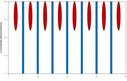
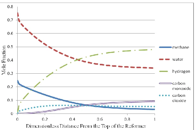
Figure 2.8. Mole fraction profile on the process-side of the SMR.
Figure 2.9. Schematic of PSA process.
Figure 2.10. Simulated mole fraction of H2 along the PSA bed during Step 1.
Figure 2.11. Simulated PSA-offgas Btu-rating
Figure 2.12. Furnace outlet temperature for a decrease in steam pressure.
Figure 2.13. Prior and posterior distributions generated by dynamic simulations
Figure 3.1. Steam-methane reforming process models.
Figure 3.2. Process model goodness-of-fit using steady-state and dynamic evaluations.
Figure 3.3. Informed prior distributions created using the four process models, as well
as the binomial likelihood distribution created using the measured alarm data.
Figure 3.4. SS1 failure probability as a function of a steam pressure decrease.
Figure 3.5. Operator response time histogram.
Figure 3.6. Operator response time as a function of temperature rate of change (plant
data and model prediction).
Figure 3.7. SS1informed prior distributions constructed using the five operator
response-time models (ORTMs) with dynamic Process Model A.
Figure 3.8. SS1 informed prior distributions constructed using the four process models
with Operator Response-Time Model E.
xiv
Figure 3.10. Informed prior distributions and associated posterior
distributions describing the failure probability of .
Figure 4.1. Alarm belt-zones and interlock shutdown for a process variable.
Figure 4.2. TPS used to generate a trial rare-event trajectory from an initial trajectory.
Figure 4.3. Boundary-value optimization to indirectly perform backward integration
using initial-value shooting.
Figure 4.4. Orthogonal collocation over finite-elements.
Figure 4.5. TPS algorithm for calculating trajectories of process safety-events.
Figure 4.6. Schematic of the exothermic CSTR.
Figure 4.7. Conversion in the exothermic CSTR.
Figure 4.8. Effect of introducing noise to an uncontrolled CSTR.
Figure 4.9. Effect of introducing noise to a controlled CSTR.
Figure 4.10. Initial rare-event trajectory.
Figure 4.11. Rare-event trajectories generated using TPS.
Figure 4.12. Example of a simulation that is too long.
Figure 4.13. First 350 TPS trajectories.
Figure 4.14. The trajectories displayed in two clusters.
Figure 4.15. Trajectory likelihood in sequence.
Figure 4.16. Number of movements between clusters as a function of perturbation size.
Figure 4.17. Probability of accepting trajectories as a function of perturbation size.
Figure 4.18. as a function of .
Figure 4.19. Concentration of A as function of temperature for all trajectories in
Cluster B.
Figure 4.20. Air Separation Unit process flow diagram.
Figure 4.21. Mole fraction profiles after LOX and LAR setpoints are increased.
Figure 4.22. Initial condition simulated data.
Figure 4.23. Clusters of rare-event trajectories.
1
Chapter 1
Introduction
1.1 Background
Despite much attention and many efforts, accidents in the chemical manufacturing
industries are relevant, costly, and occasionally fatal. In the past four years, over 100
fatalities have occurred in the United States due to a wide variety of accidents(“Worker
Fatalities to Federal and State OSHA”). There have been incidents in the past decade that
have drawn much attention due to their severe nature – BP’s Deepwater Horizon oil spill
(“U.S. Chemical Safety Board Report: BP Deepwater Horizon”), Texas City refinery
explosion (“U.S. Chemical Safety Board Report: BP America Refinery Explosion”), and
the Kleen Energy Systems explosion (“U.S. Chemical Safety Board Report: Kleen
Energy Natural Gas Explosion”), to name a few. Each of these accident scenarios
involves two critical similarities – an unexpected event occurred, and the event was not
handled properly by operators and plant managers (Kletz, 2009). Because many
chemical plants involve dangerous chemicals, high temperatures, high pressures, or are in
environmentally fragile areas (e.g., the Gulf Coast), the impacts of accidents can be quite
large. The Texas City refinery explosion claimed the lives of 14 workers and injured
over 100 more. The BP Deepwater Horizon oil spill devastated the environment along
much of the Gulf Coast, and was one of the most costly accidents ever, having damage
2
sufficiently high to warrant further research aimed at predicting, mitigating, and
preventing these accidents.
The typical approach to preventing accidents in a chemical manufacturing process
involves process design coupled with design of operating strategies, process
controlsystems, and safety systems. Processes can be designed such that they are
inherently less sensitive to disturbances in process units and feedstock fluctuations. This
approach, known as inherently safer design (ISD), often varies process-to-process, with
specific process units or features installed to handle potential accidents before they
develop (Hendershot, 2006). On the inlet of sensitive reactors, it is common for
designers to introduce buffer tanks to dampen deviations in feed flow rates, compositions,
temperatures, and pressures. Separation units commonly involve extra trays, bed depth,
or membrane areas – permitting continued operation in the face of large disturbances.
Some units are designed to be used only when a problem arises in a plant. In many cases
involving pipes designed for gas flow, a pressure-release line is installed. When the
pressure exceeds an upper bound, gas can be redirected to the release line and flared so
that it doesn’t rupture a pipe. Stop valves are typically installed on the inlet and outlet of
sensitive processing units – allowing operators to isolate problems that occur upstream of
the unit or within the unit. Various indices and statistical approaches for quantifiably
evaluating and rationalizing ISD have been developed (Srinivasan et al., 2012).
Disturbances in a plant occur on a frequent basis, often minute-to-minute, and
need to be handled in an efficient manner. While process design features can help to
dissipate disturbances, they are often not responsible for arresting them. This is the role
3
measured, and based on its deviation from its setpoint, the controller typically opens or
closes a valve in part or in full (Luyben, 1989; Stephanopoulos, 1984). Here, the
controller must be tuned properly, and the measuring device and actuator must be
functioning properly. If not, there is potential for the disturbance to propagate further.
Control configurations involving PID controllers have been developed, such as cascade
or feedforward controllers. These provide tighter and/or more robust process control,
assuming that the measuring devices and actuators are working properly.
Model-predictive controllers use first-principle or empirical models to yield actuator responses
that minimize deviations from set points over the predictive horizon (Garcia et al., 1989).
They often improve controllability, but process-model mismatch may keep controllers
from adequately arresting disturbances.
When the process design features and control systems are insufficientto regulate a
disturbance, the operator, often in response to alarms, is responsible for any corrective
actions to move the process back to typical operating conditions with a safety interlock
system shutting down the process when it deviates sufficiently far from these conditions
(Crowl et al., 2001). Operators typically have the ability to make adjustments to decision
variables in a process, open and close valves, and switch control systems on and off, and
are aided by a network of alarms. When alarms activate to notify operators that process
variables have crossed thresholds, the operators are expected to: (1) diagnose the root
cause of the problem, and (2) make appropriate corrective actions to mitigate the
consequences (Hollifield et al., 2010). This can be a difficult task, particularly when the
root cause problem is shrouded; i.e., the process is undergoing inverse response or there
4
In addition to the operator, there is an automated safety interlock system. Interlocks work
to shut down the plant automatically when specific process variables, called primary
variables, cross defined thresholds. The automatic safety interlock system is important
because it shuts down the process before safety systems, such as quench tanks or relief
valves, are activated as a last line of defense in preventing the process from entering a
runaway reaction mode where human health and environmental catastrophes are possible.
Plant operator actions are important in the continued operation of a process, and safer
operation is realized when plant operators are effective in preventing processes
from undergoing shutdown (and associated restart) and activating crucial safety
systems.
Alarms are placed on process variables to alert operators that the process is
deviating from its expected regime(s) of operation. A typical alarm has a low-threshold
(for L alarms) and a high-threshold (for H alarms) that bound the range of typical
operation. When the measured variable moves outside these thresholds, an alarm is
activated and a special-cause event has occurred. The L and H-alarm thresholds, along
with more severe alarm thresholds, are established during the commissioning phase of a
process, typically the first one to three years of operation. During the design phase,
several measured variables are chosen as primary variables. Strong candidates for
primary variables are those that best describe the safety of the process – often, the
measurements associated with the most potentially dangerous operations (i.e., process
units at high temperature or pressure, or containing hazardous chemicals). Ideally, safety
5
2009). The choice of alarm thresholds and primary variables has a major impact on the
effectiveness of the operator response to alarms to reliably maintain safe operation.
Areas of unsafe operation are commonly determined using hazard and operability,
HAZOP, analyses (Kletz, 1999). This common and systematic approach is intended to
determine all potential hazards to process units. All potential material inlets (through
designed inlet ports and backflow through outlet ports, as well as leaks through the vessel
walls) are considered, and the potential chemical reactions are postulated. Mechanical
failures to piping and valves and electrical failures to compressors, motors, and control
systems are also considered. HAZOP has long been performed as a qualitative approach,
but computer-based HAZOP approaches and algorithms have been developed, in an
effort to reduce the amount of human error that arises during the hazard identification
procedure (Venkatasubramanian et al., 1994; Palmer et al., 2008). Human error and
“safety culture” has been incorporated into HAZOP approaches, with operator mistakes
and failures studied as potential causes of hazards to process operation (Kennedy et al.,
1998). The qualitative analysis is then enhanced using quantitative statistics – the failure
rates of similar process units are used to gain an understanding of the most severe process
risks. This analysis is often the basis for determining the primary variables in the
process. Process variables associated with the greatest potential hazards or risks are
chosen as primary variables, ensuring that an automatic shutdown is attempted when
these variables are far outside their typical operating regions.
With potential hazards to process operation identified, independently-acting
safety systems are installed to maintain the probability of failure below a pre-specified
6
commonly evaluated using event-trees, where the probability of the network of safety
systems failing is the product of the failure probability of each activated safety system
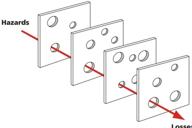
(Andrews et al., 2000; Phimister et al., 2003). As illustrated using the “Swiss Cheese
Model”, an accident occurs when the various levels of safety systems fail or are
insufficient (Reason, 1990).
Figure 1.1. Swiss cheese model
Layer of Protection Analysis (LOPA), is the industry standard to quantify the accident
probability for specific special-cause events, typically indentified during HAZOP
(Summers, 2003). This quantitative procedure is valuable in characterizing the safety of
a process during a special-cause event. More recently, techniques to evaluate the
process’s safety through a period of human error have been developed (Baybutt, 2002;
7
safety systems and the network of safety systems have been developed, all sharing the
challenge of few safety system activations over the lifetime of a process. Bayesian
networks (Marsh et al., 2008) and neural networks (Ruilin et al., 2010) have been utilized
to quantify these failure probabilities.
While LOPA estimates the probability of safety system failure, Fault Tree
Analysis (FTA) estimates the probability of special-cause event occurrence. The varying
paths leading to a special-cause event are identified and process statistics are used to
characterize the probability of such an event occurring (Khakzad et al., 2011; Tanaka et
al., 1983). These estimates can be combined with previous event-tree approaches for
analyzing the failure probability of the safety system network during a special-cause
event. This “bow-tie” approach tracks the special-cause event from its root-cause
through the safety system activation (Cockshott, 2005).
In some cases, alarms are officially considered a layer-of-protection and
contribute to the SIL rating of the overall safety system. Therefore, the alarms are
included in the safety-systems discussed herein – noting that often the full alarm system
is not considered part of a plant’s safety instrumented system (SIS). The failure
probabilities of specific safety systems, as well as the network as a whole, are often
difficult to estimate – the activation of most safety systems occur infrequently, and
oftentimes the root-cause of the event is poorly understood. If the failure probabilities of
safety systems, could be known with certainty, the probability of accidents at a process
could be guaranteed below the SIL with proper safety system design. Various techniques
and methods for quantifying the failure probabilities of rarely activated safety systems
8
Dynamic Risk Analysis (DRA) is used to update risk estimates over the lifetime
of the plant (Meel et al., 2006; Kalantarnia et al., 2009). As process and alarm data are
collected, in real-time, DRA updates the risk estimations that were made during the
design and commissioning phases. Typically Bayesian statistics (Bayesian analysis) are
used to generate failure probability estimates using alarm data (Pariyani et al., 2012a).
The Bayesian approach has the potential to generate failure probabilities having lower
variance than those achieved using classical statistics, and is explained in Chapter 2.
DRA performs best in describing the risk of frequently activated safety systems – with
more data available, estimates with narrower confidence intervals can be made. For
infrequently used systems, copulas have been introduced to make risk estimates with
smaller variances (Pariyani et al., 2012b; Yi et al., 1998). Copulas describe the
dependence between the more frequently-activated, low-consequence systems with
infrequently-activated, high-consequence systems.
While dynamic risk analysis and copulas are effective in making meaningful risk
estimates for many infrequently-used systems, data may be too sparse to permit copulas
to reduce the variance of risk estimates sufficiently. Many processes, such as the
steam-methane reformer studied herein, are well-understood, and special-cause events are
generally handled reliably by plant operators. This thesis explores model-based
approaches for better understanding the failure probabilities of operator responses to
alarms that rarely lead to safety interlock activations and associated plant shutdowns.
Process models, while not a perfect representation of the process, can be simulated many
times, generating a large pool of simulated alarm and safety interlock activations. These
9
the failure probability predictions. Various sampling techniques are developed and
applied to safety systems. In particular, this thesis explores informed prior distributions
and transition path sampling. These sampling techniques utilize both process and
operator models, enhanced by process and alarm data collected at the plant. Pathways, or
trajectories, to safety interlock activations are explored. While the safety interlock
activations investigated are inherently rare, the failures have the potential to be
catastrophic in the unlikely event that safety interlock systems fail. At best, the safety
interlock system activations are expensive due to lost product and process shutdowns.
The three chapters describing these techniques are briefly introduced in the next three
sections.
1.2 Chemical Process Simulation for Dynamic Risk Analysis: Developing Informed
Prior Distributions
Chapter 2 describes how dynamic simulations of a manufacturing process can be
used to construct informed prior distributions for the failure probabilities of alarm and
safety interlock systems. Bayesian analysis is used starting with prior distributions and
enhancing them with likelihood distributions, constructed from real-time alarm data, to
form posterior distributions, which are used to estimate failure probabilities. The use of
alarm data to build likelihood distributions has previously been investigated. Rare-event
historical data are typically sparse and have high-variance likelihood distributions. When
10
distributions, the resulting posterior distributions naturally have high variances yielding
unreliable failure predictions. In contrast with prior distributions obtained by maximizing
entropy and those that are based on expert knowledge, this chapter introduces a
repeated-simulation method to construct informed prior distributions having smaller variances,
which in turn yield posterior distributions with lower variances and a more reliable
prediction of the failure probabilities of alarm and safety interlock systems. The
application of the proposed method is demonstrated for the offline dynamic risk analysis
of a steam-methane reformer (SMR) process.
1.3 Improved Predictions of Alarm and Safety System Performance Using
Process and Operator Response-Time Modeling
In Chapter 2, a repeated-simulation process-model-based technique for
constructing informed prior distributions is introduced. The models used in simulation
are crucial to the low-variance risk predictions generated by the sampling technique.
This chapter investigates the effect modeling has on the risk predictions, and how both
process and operator models can be systematically improved to generate more accurate
risk predictions. This chapter presents a method of quantifying process model quality,
which impacts prior and posterior distributions used in Bayesian Analysis. The method
uses higher-frequency alarm and process data to select the most relevant constitutive
11
special-cause event occurrences and operators’ response-times are proposed and
validated with industrial plant data. These models can be used to improve the estimates of
failure probabilities for alarm and safety interlock systems.
1.4 Understanding Rare Safety and Reliability Events Using Transition Path
Sampling
There is strong motivation to understand how rare reliability and safety-events
develop and propagate. Effective operator training, safety system design, and safety
analysis, all benefit from a full understanding of such events. A major challenge in the
study of events that propagate to process shutdowns or safety incidents is their sparsity –
typically these events occur so rarely that statistical techniques alone are incapable of
describing and characterizing them – especially when they have not yet occurred.
Simulation of these events could be useful to understand them, however, a daunting
computational challenge exists. Typical rare events occur on the order of years or
decades apart, while the events occur within minutes or hours. Thus, the bulk of the
computational effort in simulating rare events is allocated to normal operation, making
the events computationally infeasible to simulate with meaningful frequencies.
A rare-event sampling technique, Transition Path Sampling (TPS), has been
developed by the molecular dynamics community. While the time and length scales
between molecular dynamics and process dynamics differ greatly, the ratios of the times
12
based technique relies on the simulation of perturbed rare-event trajectories – an initial
rare-event trajectory is randomly modified such that large numbers of trajectories are
generated. Clusters of rare event trajectories are the basis for alarm and
safety-system design, assuring that TPS-generated clusters are preventable. Important
modifications to the TPS technique are needed to apply it to process dynamics. The
backwards integration, a key attribute of TPS, is not possible for most process
simulations – instead a boundary-value optimization technique is used. Furthermore,
process models use vast amounts of process data for model verification and to estimate
the relative likelihood of one trajectory to another. The application of TPS is
demonstrated using a simple jacketed exothermic CSTR, as well as a more complex air
separation process. This innovative approach allows for a quantitative rationalization of
13
Chapter 2
Chemical Process Simulation for Dynamic Risk Analysis
2.1. Introduction
The design of accurate process models and optimal flowsheets have challenged
process systems engineering researchers for decades – often involving optimizations with
decision variables (such as feed-stock or operation variables) adjusted to increase
revenue, decrease cost, or increase profit (Seider et al., 2009). From a controls
perspective, controller parameters are tuned to improve performance measures (Seborg et
al., 2010). Furthermore, superstructures are used to determine which process units and
controllers should be included for optimal functionality (Yeomans et al., 1999). But,
process models and flowsheets have been under-investigated in the process safety area,
where process engineers are challenged to reduce the risk of incidents, the most serious
of which may be classified as accidents. Process incidents, resulting in human-health
losses, environmental losses, and capital losses, are expensive and occasionally tragic
(when safety systems are insufficient to prevent process incidents from becoming process
accidents) (U.S. Chemical Safety and Hazard Investigation Board; Process Safety
Incident Database).
To design and operate a process with reduced incident and accident risk, it is
crucial to quantify the probabilities of incidents. This can be a difficult task, as it
14
probability of each consequence arising from each special cause, and (3) evaluating the
severity of each consequence(Pariyani et al., 2010; Mannan et al., 1999). To quantify
accurately the overall risk of an incident, these three tasks are required for every special
cause, consequence, and loss, providing quite a daunting challenge! The success or
failure of an alarm system depends upon the success or failure of operator actions taken
in response to an activated alarm. In contrast, the Safety Instrumented System (SIS)
takes automatic actions such as a shutdown initiated by an interlock. In this paper, the
focus is on simulating the effects of special cause events to inform and improve design
and operation decisions to mitigate incidents. In this manner, process engineers and
operators can make more informed decisions to reduce plant risk (Phimister et al., 2003;
Jones et al., 1999).
Emphasis is placed on constructing sufficiently accurate process simulations to
evaluate plant safety, given measured process and alarm data. Clearly, special attention
is needed: (i) in the most risky plant areas, and (ii) when special-cause events are likely to
be amplified or masked (Rosenthal et al., 2006). The former typically involve high
temperatures, pressures, and hazardous chemicals. The latter are more difficult to
identify, especially when their responses occur in rapid transients. Masked responses
include inverse responses and delays (dead-times) which may lead operators to take
incorrect action in response to alarms. Here, dynamic, first-principles, process models,
built with knowledge from historical process and alarm data(Chen et al., 1998), can help
operators respond better to these special-causes. While first-principles models have long
15
(Soroush et al., 1992), this paper provides a new method to estimate the failure
probabilities of alarm and safety interlock systems.
The rest of this chapter begins with a discussion of typical alarm and safety
interlock systems and their associated event trees and failure probabilities. Next,
Bayesian analysis is reviewed, followed by the presentation of a new method that uses
dynamic simulations to create informed prior distributions for Bayesian analysis. Then, a
detailed steam-methane reforming (SMR) model integrated with a pressure-swing
adsorption (PSA) model is presented and the proposed method is demonstrated by
simulating the combined model. To our knowledge, no published integrated SMR-PSA
model exists including recycle of the PSA-offgas to the SMR fuel system. Finally,
conclusions are drawn with recommendations for future work.
2.2. Safety Systems and Event Trees
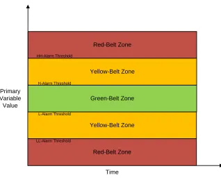
An abnormal event occurs when a process variable leaves its normal operating
range (green-belt zone in Figure 2.1), which triggers an alarm indicating transition into
the yellow-belt zone. If the variable continues to move away from its normal range, the
variable may transition into its red-belt zone, indicated by a second-level alarm (e.g., LL,
HH) activation. Once a variable remains in its red-belt zone for a pre-specified length of
time (typically on the order of seconds), an interlock activates and an automatic shutdown
16
Green-Belt Zone Red-Belt Zone
Yellow-Belt Zone
Time Primary
Variable Value
H-Alarm Threshold HH-Alarm Threshold
Yellow-Belt Zone
Red-Belt Zone L-Alarm Threshold
LL-Alarm Threshold
Figure 2.1. Belt-zone map for primary variables.
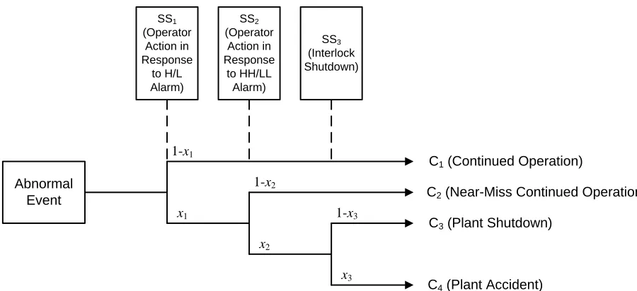
An event-tree corresponding to a primary variable’s transition between belt-zones
is shown in Figure 2.2. The first-level (e.g., L, H) alarm system activates safety-system 1
(SS1), which is typically an operator action. When SS1 is successful, with probability
1-x1, continued operation, consequence C1, is achieved. The second-level (e.g., LL, HH)
alarm system activates SS2, which is typically a more aggressive operator action. When
successful, with probability 1-x2, near-miss continued operation, consequence C2, is
achieved. If the primary variable occupies the red-belt zone for a pre-determined length
of time (on the order of seconds), SS3, the automatic interlock plant shutdown, will
become activated. The interlock system is designed to be independent of alarm systems,
and the activation of SS3 is determined by an independent set of sensors. It should be
17
success is equal to zero (x2 = 1). If SS3 succeeds, with probability 1-x3, the interlock
shutdown is successful and an accident is avoided, represented by consequence C3. If the
interlock shutdown is unsuccessful, an accident occurs at the plant, represented by C4.
With proper design, x3 should be very small consistent with the specified Safety Integrity
Level (SIL) (Stavrianidis et al., 1998; Stavrianidis et al., 2000). Since the interlock
system is independent of the alarm system, the success of SS3 will not depend on factors
such as operator skill or alarm sensor fault. However, it can be concluded that if either
SS1 or SS2 are successful in arresting the special-cause event, the activation of the
interlock system can be avoided altogether. In some cases, alarms are officially
considered a layer-of-protection and contribute to the SIL rating of the overall safety
system, composed of SS1, SS2, and SS3. Therefore, the alarms are included in the
safety-systems herein – noting that often the full alarm system is not considered part of a plant’s
SIS.
In this way, event trees represent the actions of various alarm and safety interlock
systems and their end consequences after abnormal events (Meel et al., 2006). For
dynamic risk analyses, alarm and interlock actions must be chronologically tracked and
recorded (using the plant alarm historian). Using data compaction techniques and
Bayesian analyses, failure probabilities of the alarm and safety interlock systems and the
probabilities of plant incidents(Pariyani et al., 2012a; Pariyani et al., 2012b) have been
18 Abnormal Event SS1 (Operator Action in Response to H/L Alarm) SS2 (Operator Action in Response to HH/LL Alarm) SS3 (Interlock Shutdown)
C1 (Continued Operation)
C2 (Near-Miss Continued Operation)
C4 (Plant Accident)
C3 (Plant Shutdown)
1-x1
1-x2
1-x3 x1
x2
x3
Figure 2.2. Event tree involving three safety systems.
2.3. Bayesian Analysis
Bayesian analysis is often used to determine the failure probabilities of alarm and
safety interlock systems. The central dogma of Bayesian analysis is that random-variable
distribution parameters (e.g., mean and variance) are themselves distributions. Unlike
classical statistics that seeks to capture the true moments of a distribution, Bayesian
statistics acknowledges that the moments of a distribution may not be fixed, and seeks to
estimate the probability distributions of the moments. This analysis often requires
significantly fewer data to make meaningful predictions (Gelman et al., 2014; Berger,
2013). Additionally, as the process dynamics and operators’ behavior change with time
real-19
time data can be collected and used to estimate more accurate failure probabilities in real
time.
In Bayesian analysis, the posterior distribution, represented as , the
probability distribution of given the collected data, , is calculated using
Bayes’ rule:
(2.1)
where is the prior distribution of , estimated before data are collected, and
is the likelihood distribution of the data given . The prior distribution is
normally estimated using expert knowledge or maximum entropy techniques (Ahooyi et
al., 2014). The likelihood distribution captures the probability that the data could have
been generated, if the failure probability was equal to , as discussed next.
Herein. a beta distribution is used to represent an informed prior distribution,
which is constructed using process simulations:
(2.2)
where and are parameters obtained through simulation, and is the gamma
20
(2.3)
The beta distribution is well suited to represent a safety-system failure-probability
distribution because its domain is [0, 1], and its two parameters can be estimated from
only two moments (e.g., the mean and variance) of simulated data.
The alarm data provides a record of each safety system activation, which can be tracked
to its failure or success. The binary performance lends itself to being described using a
binomial likelihood distribution:
(2.4)
where represents the alarm data, is the number of safety system activations, and is
the number of safety system failures. When Eqs. (2.2) and (2.4) are substituted into Eq.
(2.1), the posterior distribution for , given and is:
(2.5)
This is a beta distribution with parameters and ,
recognizing that is a function of only. Note that for the beta distribution in Eq. (2.2),
21
(2.6)
the posterior distribution in Eq. (2.5) simplifiesto thebeta distribution:
(2.7)
As alarm data are collected in real time, the alarm statistics can be updated in real time
(Meel et al., 2006; Khakzad et al., 2012; Kalantarnia et al., 2009). In so doing, process
engineers gain a better understanding of how the process is performing (Pariyani et al.,
2012b).
2.4. Constructing Informed Prior Distributions
The proposed method of construction of informed prior distributions has the eight
steps listed in Table 1. In Steps 1-3, a robust, dynamic, first-principles model of the
process incorporating the control, alarm and safety interlock systems, is built. The model
can then be simulated using a simulator such as gPROMS (gPROMS v.3.6.1; Oh, et. al.,
1996), which is used herein. The control system in the model mimics the actual plant
22
interlock systems in the model mimic those in the plant. For operator actions, this can be
difficult, as operators often react differently to alarms. In particular, expert operators
may take into account the state of the entire process when responding to alarms. When
creating a model, the likelihood of operator actions must be considered. Either the
modeler can use the action most commonly taken by operators, or a stochastic simulation
can be set up in which the different actions are assigned probabilities.
With these models, special-cause events are postulated in Step 4. The list of
special-cause events can be developed from various sources: HAZOP or LOPA analysis,
observed accidents in the plant (or a similar plant), near-miss events at the plant (or in a
similar plant), or from risks suggested in first-principles models of the plant. For each
special-cause event, an event magnitude distribution is created in Step 5. A distribution
for operator response time, τ, is created in Step 6. These three distributions are used
along with the dynamic simulation in Step 7 to obtain simulation data. Lastly, in Step 8,
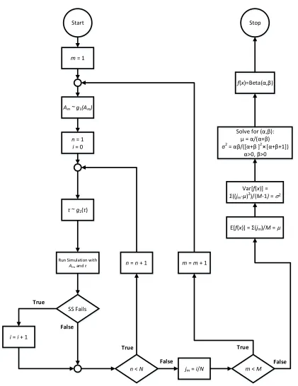
the simulated data is used to regress parameters for the informed prior distribution. The
algorithm used to generate simulation data (Step 7) and regress informed prior
distribution parameters (Step 8) is described in the paragraph below, and represented
pictorially in Figure 2.3.
The script that manages the dynamic simulations starts by sampling A1 from the
event magnitude distribution created in Step 5. Note that Figure 2.3 shows a Normal
distribution centered at µSC with variance σ2SC, however any distribution can be used.
Assign the number of safety system failures, i, to i = 0. With this A1, the user script
samples τ1 from the distributions created in Step 6. Although Figure 2.3 shows Uniform
23
used. With A1 and τ1, a dynamic simulation is run. If the safety system fails to avoid a
plantwide shutdown, then i = i + 1; if the safety system is successful, i is not incremented.
When n < N, n = n + 1; i.e., for sampled Aiand τi, a dynamic simulation is run, and i is
adjusted when necessary. After N iterations, j1 = i/N is calculated, in the range [0,1].
Then m is incremented and Am sampled, the inner loop is re-executed, and jm is calculated.
When the outer loop has been completed (m = M), a vector of M elements (j1, ..., jM) has
been accumulated. The average and variance of this vector is used to calculate and of
the Beta distribution. Note that because the Beta distribution is the conjugate prior of the
binomial likelihood distribution, it is the recommended choice. The number of
simulations, M×N, is chosen, recognizing that more simulations yield a smaller
prior-distribution variance.
Table 2.1. Steps to Construct an Informed Prior Distribution
1. Develop a dynamic first-principles process model
2. Incorporate control system into the dynamic process model
3. Incorporate the alarm and safety interlock system into the dynamic process
model
4. Postulate potential special-cause events to be studied
5. For each special-cause event, construct a distribution for the event
magnitudes, ASC (i.e., for a postulated pressure decrease, construct a probability
distribution for a decreasing magnitude)
6. For each special-cause event, construct a distribution for operator response
time, τ.
7. For each special-cause event, conduct the simulation study according to
the algorithm described in Figure 2.3 to simulate the range of possible event
24
8. Estimate parameters of a distribution model (e.g., Beta distribution)
representing the data generated in Step 7 – this is used as an informed prior
25
Start
m = 1
Am ~ g1(Am)
n = 1
i = 0
τ ~ g2(τ)
Run Simulation with
Am, and τ
SS Fails
i = i + 1
n < N n = n + 1
jm = i/N m < M
m = m + 1
E[f(x)]=Σ(jm)/M =μ
Var[f(x)]= Σ((jm-μ)2)/(M-1) =σ2
Solve for (α,β): μ = α/(α+β) σ2 = αβ/([α+β ]2⨯[α+β+1])
α>0, β>0
f(x)=Beta(α,β) Stop
True
True True
False
False False
26
2.5. Steam-Methane Reforming (SMR) Process
A typical SMR process is shown in Figure 2.4. After pretreatment, natural gas
feed (70) and steam (560) are mixed before entering the process tubes of an SMR unit
(90), where hydrogen, carbon monoxide, and carbon dioxide are produced. This hot
process gas (100) is then cooled and sent to a water-gas shift converter (110), where
carbon monoxide and water are converted to hydrogen and carbon dioxide. The process
gas effluent (120) is cooled in another heat exchanger, producing stream 170, which is
sent to two water extractors. Note that the last section of this heat exchanger is used to
transfer heat to a boiler feed water makeup stream in an adjacent process. The gaseous
hydrogen, methane, carbon dioxide, and carbon monoxide, in stream 210, are sent to PSA
beds. Here, high-purity hydrogen is produced (220), and the PSA-offgas is sent to a
surge drum. Stream 800 from the surge drum is mixed with hot air (830) and a small
amount of natural gas makeup (815), and sent to the furnace side, where it is combusted
to provide heat to the highly-endothermic process-side reactions. Its hot stack gas (840)
is sent through an economizer, where it is used to heat steam (520), some of which is
used on the process side (560), with the rest available for use or sale as a steam product
27
Figure 2.4. SMR process flow diagram
In modeling for process safety, emphasis should be placed on units that present
the greatest risk; i.e., have the largest probabilities of incidents multiplied by incident cost
(Kalantamia et al., 2009). In an SMR process, temperatures rise above 1,300 K with
pressures over 20 atm. Because overheating can lead to process-tube damage and failure,
potentially leading to safety concerns, its model received special attention in this work.
Partial differential and algebraic equations (PDAE’s), that is, momentum, energy and
species balances, accounted for variations of pressure, temperature, and composition in
the axial direction for both the process- and furnace-side gases. For the reforming tubes,
the rigorous kinetic model (Xu et al., 1989)was used, while the furnace-gas combustion
reactions were modeled using a parabolic heat-release profile. Convection and radiation
28
simulations and gray-gas assumptions. The heat transfer on the process side was
modeled by convection only, assuming a pseudo steady-state between the process gas and
catalyst. Details of the models are Section 2.6.
The PSA beds represent a cyclic process, with beds switched from adsorption to
regeneration on the order of every minute. This type of separation scheme induces
oscillatory behavior throughout the SMR process. As the flow rates, compositions, and
pressures fluctuate in effluent streams from the PSA beds, variables throughout the entire
plant fluctuate as well. In processes with such cyclical units, buffer tanks are often used
to dampen fluctuations. However, typical buffer-tank sizes (comparable to SMR-unit
sizes) reduce the amplitude of these fluctuations by on the order of 50%. Herein, the
SMR process test-bed involves four PSA beds, which operate in a 4-mode scheme, with
each bed undergoing adsorption, depressurization, desorption, and repressurization steps.
PDAE’s are used to model the momentum, energy, and species balances, dynamically
tracking pressure, temperature, and composition in the axial direction. Langmuir
isotherms are used to model adsorption kinetics. Details of the models are in Section 2.7.
In the full safety process model, the SMR-unit and PSA-bed models are used in
conjunction with dynamic models for the water-gas shift reactor, water extractor, surge
tank, heat exchanger, and steam drum. Furthermore, the controls used with the dynamic
process model are consistent with those used in the real process. The full process is
modeled using the software package, gPROMS. A challenging aspect of the full process
29
To my knowledge, no published SMR model exists with this level of detail. In particular,
this process model combines SMR and PSA-bed units within a plant-wide scheme with
PSA-offgas recycle. The results computed by gPROMS are consistent with the process
data from the industrial plant. This plant-wide model is extremely useful for building
leading indicators and prior distributions of alarm and safety interlock system failure
probabilities.
With a dynamic process model, process engineers can simulate special cause
events and track variable trajectories. Consider an unmeasured 10 percent decrease in the
Btu-rating, due to a composition change of the natural gas feed (40), in Figure 2.4. Note
that the makeup stream (815) on the furnace side is relatively small and is not changed in
the simulation. Initially, because the process stream contains less carbon, less H2 is
produced. Because these reactions are endothermic, less heat from the furnace is
consumed by the reactions and the furnace temperature rises, as shown in Figure 2.5.
Also, the process-side temperature increases. Eventually, the low-carbon PSA-offgas
reaches the SMR furnace. With less methane for combustion, the furnace temperature
decreases, as does the temperature of the process gas. This effect is shown in Figure 2.5.
Note that the temperatures oscillate due the natural gas oscillation in stream 800 from the
30
Figure 2.5. SMR effluent temperatures for a 10% decrease in the Btu
content of the natural gas feed.
2.5.1. Reformer Model
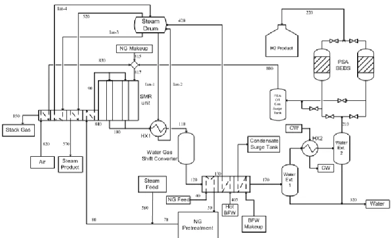
The SMR herein is a top-fired unit consisting of approximately 400 process tubes.
Steam and CH4 are fed on the process side (Stream 90 in Figure 2.4). In the tubes, H2 is
produced via a set of endothermic reactions. On the furnace side, a fuel source (Stream
817) is combusted to provide heat for the process side. A schematic of the SMR unit is
31 Tube Flame x-coordinate [dimensionless] 100 25 50 75 0
0 25 50 75 100
y -c o o rd in a te [ d im e n s io n le s s ]
Figure 2.6. Front-view schematic of SMR.
The model proposed by (Latham et al., 2011), which describes the SMR in the
steady-state, was converted to a dynamic model. Also, for the furnace-side, radiation view
factors replaced the software RADEX used by Latham. In this work, the SMR is
modeled as four units: the process gas, the process tubes, the furnace gas, and the
reformer brick. The process gas and the furnace gas are modeled as networks of
PDAE’s, having derivatives with respect to time ( ) and axial direction ( ). Each model
is discretized in the axial direction with central-difference approximations. The resulting
32
at the end of each time step. The process tubes and reformer brick are modeled as
networks of PDAE’s, having derivatives with respect to time ( ), axial direction ( ), and
lateral direction (y). These are also discretized in the spatial coordinates with central
difference approximations.
In the process and furnace gas models, the state variables are the molar flow rates of each
species i ( ) and temperature ( ). For the process gas, the mass balances for species i
are:
(2.8)
and the energy balance is:
(2.9)
where is the concentration of species i, AC is the cross-sectional area of a process tube,
is the stoichiometric coefficient of species i in reaction j, Cv is the molar heat capacity
at constant volume, Cp is the molar heat capacity at constant pressure, h is the
heat-transfer coefficient, r is the inner tube radius, Ttube is the tube wall temperature, and
is the enthalpy of reaction j. The heat capacities are functions of Ci, which are functions
of and :
33
(2.11)
(2.12)
These functions are used in Eqs. (2.8) and (2.9).
The reaction rates are calculated using the kinetic model of (Xu et al., 1989),
which involves three reforming reactions:
(R2.1)
(R2.2)
(R2.3)
The reaction rates are:
(2.13)
(2.14)
(2.15)