The Bakery

The Bakery

ABSTRACT

Three cases that focus on a bakery are presented. These cases are ideal for use in a statistics class to assess how well students have mastered descriptive statistics, probability distributions, and statistical inference. Case 1 focuses on descriptive statistics including tables, graphs, numerical measures, grouped data, and covariance and correlation. Case 2 focuses on the binomial, the Poisson, and the normal probability distributions. Finally, Case 3 focuses on confidence intervals and hypothesis testing. A solution for each case is provided.

Keywords: Descriptive Statistics; Probability Distributions; Statistical Inference; Statistics Cases; Business Case Study

OVERVIEW

he following three cases focus on a bakery. The first case deals with descriptive statistics where students are asked to create different types of tables and graphs, calculate numerical measures for grouped and ungrouped data, discuss the type of relationship between two variables, and to provide observations and recommendations. The second case focuses on the binomial, the Poisson, and normal probability distributions. Finally, the third case focuses on statistical inference where students are asked to construct confidence intervals, run different types of hypothesis tests, and to provide observations and recommendations.

CASE 1: DESCRIPTIVE STATISTICS

Emily has recently taken over her grandparent’s bakery business. She is learning the new business and wants to continue the past success of the bakery which has been in her family for over fifty years. Currently, the bakery’s primary products are bread, cakes, cookies, cupcakes, doughnuts, muffins, pies, and rolls.

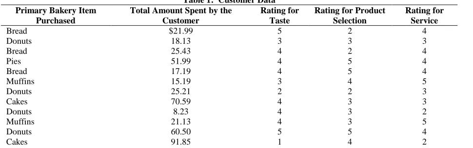
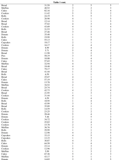
Emily is curious to see which bakery products are the most popular, the amount a typical customer spends, and how customers would rate the bakery on taste, product selection, and service. Emily decides to track the primary bakery items purchased and the amount customers spend. In addition, she asks these customers to rate the tastiness of the bakery’s products, selection, and service on a scale from one to five with five being the highest and one the lowest. Table 1 shows the data for 75 customers surveyed. For example, Customer 4’s main purchase was pies, the customer spent $51.99, and gave taste a 4, selection a 5, and service a 4.

Table 1: Customer Data Primary Bakery Item

Purchased

Total Amount Spent by the Customer

Rating for Taste

Rating for Product Selection

Rating for Service

Bread $21.99 5 2 4

Donuts 18.13 3 3 3

Bread 25.43 4 2 4

Pies 51.99 4 5 4

Bread 17.19 4 5 4

Muffins 15.19 3 4 5

Donuts 25.21 2 2 3

Cakes 70.59 4 3 3

Donuts 8.23 4 3 2

Muffins 21.13 4 3 5

Donuts 60.50 5 5 4

Cakes 91.85 1 4 2

Table 1 cont.

Bread 31.59 2 5 5

Muffins 40.52 3 2 3

Cakes 82.16 2 2 4

Cookies 11.42 5 5 2

Rolls 24.19 5 5 3

Cookies 20.90 4 1 5

Bread 12.14 3 1 5

Bread 37.62 4 3 4

Cookies 43.69 4 5 4

Rolls 31.53 3 1 1

Bread 27.46 3 2 3

Donuts 35.48 1 5 4

Rolls 19.99 1 5 2

Cakes 55.13 1 5 2

Cupcakes 18.17 2 1 1

Cookies 16.17 4 4 2

Donuts 8.99 2 4 1

Donuts 5.71 5 4 1

Bread 11.98 3 2 2

Pies 58.19 3 5 2

Donuts 10.08 1 4 3

Cakes 57.63 5 5 3

Muffins 32.94 4 5 4

Bread 18.48 4 2 5

Cakes 79.17 3 2 4

Bread 41.44 1 1 5

Rolls 6.59 1 1 2

Bread 25.67 4 1 4

Cakes 57.19 5 5 3

Donuts 13.78 3 2 1

Muffins 34.52 2 1 3

Bread 25.74 1 1 3

Cookies 42.73 4 2 4

Bread 21.95 1 3 1

Cookies 31.44 4 1 2

Donuts 6.59 2 4 1

Rolls 18.95 1 4 4

Bread 43.99 3 3 3

Bread 35.89 4 1 2

Rolls 14.59 4 1 5

Cookies 23.25 2 2 5

Donuts 28.46 5 4 3

Donuts 5.46 2 5 3

Cookies 34.72 5 1 5

Cookies 25.83 2 4 2

Cookies 15.78 2 3 5

Muffins 36.76 3 3 5

Rolls 29.99 1 1 3

Donuts 12.98 4 2 5

Cupcakes 33.15 4 5 1

Cupcakes 12.15 1 3 3

Rolls 30.87 4 3 5

Cakes 64.58 5 4 5

Donuts 23.14 1 3 4

Cookies 12.96 5 2 2

Muffins 5.99 1 3 2

Cakes 67.36 5 2 3

Muffins 43.17 5 1 1

Table 1 cont.

Cookies 43.42 3 2 3

Cookies 17.55 2 5 3

Bread 12.55 4 3 3

Rolls 40.18 4 2 1

In addition, Emily would like to know how her bakery compares with others. She contacts her cousin, who runs a bakery in another town that sells similar bakery items. Her cousin sends her customer data that is grouped. However, Emily can find estimates for measures such as the mean and standard deviation. Table 2 contains the frequency distribution of the total amount spent by customers. For example, 13 customers spent between $30.00 to $39.99.

Table 2: Total Amount Spent by Customers

Class Frequency

$ 0.00 to $ 9.99 4

$10.00 to $19.99 18

$20.00 to $29.99 20

$30.00 to $39.99 13

$40.00 to $49.99 3

$50.00 to $59.99 5

$60.00 to $69.99 4

$70.00 to $79.99 5

$80.00 to $89.99 2

$90.00 to $99.99 1

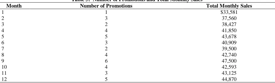
Finally, Emily notices that the bakery usually does monthly promotions and wants to know if there is truly a relationship between the number of promotions and total sales. She gathers data from the past twelve months. Table 3 below provides the number of promotions and total sales for the past twelve months. For example, in Month 3 the total number of promotions was 2 and the total monthly sales was $38,427.

Table 3: Number of Promotions and Total Monthly Sales

Month Number of Promotions Total Monthly Sales

1 1 $33,581

2 3 37,560

3 2 38,427

4 4 41,850

5 5 43,678

6 3 40,909

7 2 39,500

8 4 42,740

9 6 47,500

10 4 42,593

11 3 43,125

12 5 44,870

Now that Emily has all this data, she needs some help organizing and analyzing it. She would like the following included in a report:

1) Primary bakery item purchased (Table 1)

 Construct a frequency distribution and relative frequency distribution for the data.  Construct a bar graph and pie chart.

 Discuss the results of the tables and charts.

2) Total amount spent by customers (Table 1)

 Determine the following numerical measures: mean, median, mode, range, sample variance, sample standard deviation, first quartile, third quartile, interquartile range, sample skewness, and the coefficient of variation.

 Discuss the results of the tables, histogram, and numerical measures.  Discuss the shape of the data using both graphical and numerical measures.

3) Grouped data (Table 2)

 Determine the mean and standard deviation for the grouped data.

 Discuss how these numerical measures compare to those found for the total amount spent by customers at Emily’s bakery (Table 1 data). How are they different?

4) Ratings for taste, product selection, and service (Table 1)

 Summarize in a table the ratings for taste, product selection, and service.  Determine the weighted average for each.

 Discuss the findings. Are there areas for improvement?

5) Total Sales vs. Number of Promotions (Table 3)

 Construct a scatter diagram for the total sales and the number of promotions data.  Determine the sample covariance and the sample correlation between these variables.

 Discuss the results of the scatter diagram and covariance and correlation calculations. Be sure to include a discussion of the type of relationship that exists between the two variables.

CASE 2: PROBABILITY DISTRIBUTIONS

Emily has recently taken over her grandparent’s bakery business. She is learning the new business and wants to continue the past success of the bakery which has been in her family for over fifty years. The bakery’s primary products are bread, cakes, cookies, cupcakes, doughnuts, muffins, pies, and rolls.

Emily’s new baker has been trying some new muffin recipes. She is curious to see how many of a batch of 24 will remain at the end of the day. Suppose that the number of muffins remaining at the end of the day follows a binomial distribution and that there is a 15% chance that a muffin will not be purchased by the end of the day. Help Emily determine the following:

1) The expected number and standard deviation of muffins remaining. 2) The probability that all muffins will be sold.

3) The probability that five muffins will remain. 4) The probability that three or less muffins will remain. 5) The probability that more than five muffins will remain.

6) The probability that more than three, but less than eight muffins will remain.

In addition, Emily is curious about the number of people entering her bakery over a half-hour period. Suppose that customer arrivals follow a Poisson distribution and that on average 10.5 customers enter the store every 30 minutes. Help Emily determine the following:

1) The probability that ten customers will enter the store in the next 30 minutes.

2) The probability that seven or more customers will enter the store in the next 30 minutes. 3) The probability that less than five customers will enter the store in the next 30 minutes.

4) The probability that between eight and twelve customers will enter the store in the next 30 minutes.

5) The probability that more than eight, but less than fourteen customers will enter the store in the next 30 minutes.

1) The probability that total daily sales will be more than $2000. 2) The probability that total daily sales will be less than $1300.

3) The probability that total daily sales will be between $1250 and $1800. 4) The probability that total daily sales will be between $1750 and $2100.

5) Determine the amount where there is a 30% chance that total daily sales will be less than this amount. 6) Determine the amount where there is a 95% chance that total daily sales will be above this amount.

CASE 3: STATISTICAL INFERENCE

Emily has recently taken over her grandparent’s bakery business. She is learning the new business and wants to continue the past success of the bakery which has been in her family for over fifty years. Currently, the bakery’s primary products are bread, cakes, cookies, cupcakes, doughnuts, muffins, pies, and rolls.

Emily is curious to see what the average daily sales are at her store. She believes that it is around $1600. Emily collects data from the past 50 days. Table 4 below displays the total daily sales for the past fifty days. Assume this data comes from a normally distributed population where the population standard deviation is unknown.

Table 4: Total Daily Sales

$1,800 $975 $1,814 $1,421 $1,335

$1,273 $1,592 $1,305 $1,103 $1,105

$1,438 $1,219 $1,661 $1,692 $1,709

$1,584 $1,111 $1,613 $1,547 $1,715

$1,384 $1,595 $1,139 $2,017 $2,014

$1,497 $1,820 $1,770 $1,799 $1,386

$1,368 $1,506 $1,852 $1,642 $1,355

$1,199 $1,416 $1,716 $982 $1,851

$1,649 $1,864 $1,532 $1,318 $1,367

$1,939 $1,384 $1,867 $1,389 $1,152

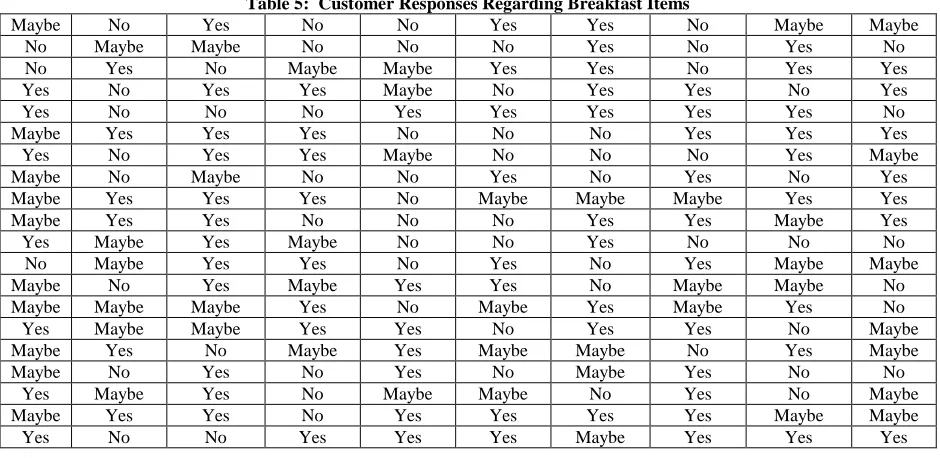
In addition, Emily is wondering whether she should add additional breakfast items such as French toast and egg sandwiches. There are many businesses in the downtown area near her bakery so this may provide quick breakfast solutions for people on their way to work. She believes that half of her customers will purchase breakfast items. Emily asks 200 customers whether they would purchase breakfast items if they were available. Table 5 provides the customer responses of Yes, No, and Maybe.

Table 5: Customer Responses Regarding Breakfast Items

Maybe No Yes No No Yes Yes No Maybe Maybe

No Maybe Maybe No No No Yes No Yes No

No Yes No Maybe Maybe Yes Yes No Yes Yes

Yes No Yes Yes Maybe No Yes Yes No Yes

Yes No No No Yes Yes Yes Yes Yes No

Maybe Yes Yes Yes No No No Yes Yes Yes

Yes No Yes Yes Maybe No No No Yes Maybe

Maybe No Maybe No No Yes No Yes No Yes

Maybe Yes Yes Yes No Maybe Maybe Maybe Yes Yes

Maybe Yes Yes No No No Yes Yes Maybe Yes

Yes Maybe Yes Maybe No No Yes No No No

No Maybe Yes Yes No Yes No Yes Maybe Maybe

Maybe No Yes Maybe Yes Yes No Maybe Maybe No

Maybe Maybe Maybe Yes No Maybe Yes Maybe Yes No

Yes Maybe Maybe Yes Yes No Yes Yes No Maybe

Maybe Yes No Maybe Yes Maybe Maybe No Yes Maybe

Maybe No Yes No Yes No Maybe Yes No No

Yes Maybe Yes No Maybe Maybe No Yes No Maybe

Maybe Yes Yes No Yes Yes Yes Yes Maybe Maybe

Now that Emily has all this data she would like some help with the following:

1) Construct 90%, 95%, and 99% confidence intervals for the population mean of total daily sales.

2) Run a hypothesis test on the population mean for total daily sales. Use a hypothesized value of $1600 and test at levels of significance of 0.01, 0.05, and 0.10. Use both the critical value and p-value approaches when testing at each level of significance.

3) Run another hypothesis test on what you believe is the true average total daily sales at the bakery. Test at levels of significance of 0.01, 0.05, and 0.10. Use the critical value and p-value approaches when testing at each level of significance.

4) Construct 90%, 95%, and 99% confidence intervals for the population proportion of those that will definitely purchase breakfast items (Yes response).

5) Run a hypothesis test on the population proportion of those that will definitely purchase breakfast items (Yes response). Use a hypothesized value of 0.50 and test at levels of significance of 0.01, 0.05, and 0.10. Use both the critical value and p-value approaches when testing at each level of significance.

6) Run a hypothesis test on what you believe is the true proportion of people who will definitely purchase breakfast items (Yes response). Test at levels of significance of 0.01, 0.05, and 0.10. Use the critical value and p-value approaches when testing at each level of significance.

Finally, Emily would like her report to include observations and recommendations based on the results of the confidence intervals and hypothesis tests for the population mean and population proportion.

CASE 1 SOLUTION

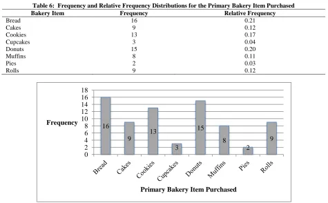
The following is a possible solution for Case 1. Table 6 shows the frequency and relative frequency distributions and Figures 1 and 2 show the bar graph and pie chart for the primary bakery item purchased. The data can be found in Table 1. It appears that bread, donuts, and cookies are the primary bakery items purchased by customers. Cupcakes and pies are the least primary bakery items purchased by customers.

Table 6: Frequency and Relative Frequency Distributions for the Primary Bakery Item Purchased

Bakery Item Frequency Relative Frequency

Bread 16 0.21

Cakes 9 0.12

Cookies 13 0.17

Cupcakes 3 0.04

Donuts 15 0.20

Muffins 8 0.11

Pies 2 0.03

Rolls 9 0.12

Figure 1: Bar Graph for the Primary Bakery Item Purchased 16

9

13

3

15 8

2

9

0 2 4 6 8 10 12 14 16 18

Frequency

Figure 2: Pie Chart for the Primary Bakery Item Purchased

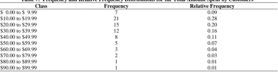
Table 7 shows the frequency and relative frequency distributions and Figure 3 shows the histogram for the total amount spent by customers. The data can be found in Table 1. The mean is $30.33, the median is $25.67, the mode is 6.59, the sample variance is 381.21, the sample standard deviation is 19.52, sample skewness is 1.11, the range is 86.39, the first quartile is 15.19, the third quartile is 40.52, the interquartile range is 25.33, and the coefficient of variation is 0.64. According to the table and histogram the majority of the customers tend to spend between $10.00 to $39.99 at the bakery. The shape of the data appears to be skewed to the right since Figure 3 shows a long right tail, the sample skewness is positive, and the mean is larger than the median. The grouped data in Table 2 results in a sample mean of $34.06 and a sample standard deviation of $21.82. These are approximations since the individual customer total sales were not given.

Table 7: Frequency and Relative Frequency Distributions for the Total Amount Spent by Customers

Class Frequency Relative Frequency

$ 0.00 to $ 9.99 7 0.09

$10.00 to $19.99 21 0.28

$20.00 to $29.99 15 0.20

$30.00 to $39.99 12 0.16

$40.00 to $49.99 8 0.11

$50.00 to $59.99 5 0.07

$60.00 to $69.99 3 0.04

$70.00 to $79.99 2 0.03

$80.00 to $89.99 1 0.01

$90.00 to $99.99 1 0.01

Bread 21%

Cakes 12%

Cookies 17%

Cupcakes 4% Donuts

20% Muffins

11% Pies

3%

Rolls 12%

Bread

Cakes

Cookies

Cupcakes

Donuts

Muffins

Pies

Figure 3: Histogram for the Total Amount Spent by Customers

Table 8 summarizes the number of customers that gave a rating of 1, 2, 3, 4, or 5 for taste, product selection, and service at the bakery. This data can be found in Table 1. The weighted average is 3.09 for taste, 2.96 for product selection, and 3.17 for service. It appears that all three areas could be improved.

Table 8: Ratings for Taste, Product Selection, and Service

Rating Taste Product Selection Service

1 14 15 10

2 13 18 14

3 13 14 20

4 22 11 15

5 13 17 16

Figure 4 depicts a scatter diagram for monthly sales vs. the number of promotions. This data can be found in Table 3. The sample covariance is 4865.77 and the sample correlation coefficient is 0.9131. According to the scatter diagram in Figure 4 and the numerical measures, it appears that there is a positive linear relationship between the number of promotions and monthly sales. The graph shows an upward linear trend. Both the sample covariance and sample correlation are positive and the correlation coefficient is very close to +1.

Figure 4: Monthly Sales vs. Number of Promotions 7 21 15 12 8 5

3 ₂

1 1

0 5 10 15 20 25 $0 to $9.99 $10.00 to $19.99 $20.00 to $29.99 $30.00 to $39.99 $40.00 to $49.99 $50.00 to $59.99 $60.00 to $69.99 $70.00 to $79.99 $80.00 to $89.99 $90.00 to $99.99 Frequency

Total Amount Spent by Customers

$30,000 $32,000 $34,000 $36,000 $38,000 $40,000 $42,000 $44,000 $46,000 $48,000 $50,000

0 2 4 6 8

Monthly Sales

CASE 2 SOLUTION

The following is the solution for the binomial, Poisson, and normal probability distribution problems found in Case 2.

Binomial:

1) The expected number of muffins remaining is (24)(0.15) = 3.60

The standard deviation is 2) The probability that all muffins will be sold:

3) The probability that five muffins will remain:

4) The probability that three or less muffins will remain:

5) The probability that more than five muffins will remain:

6) The probability that more than three, but less than eight muffins will remain:

Poisson:

1) The probability that ten customers will enter the store in the next 30 minutes:

2) The probability that seven or more customers will enter the store in the next 30 minutes:

3) The probability that less than five customers will enter the store in the next 30 minutes:

4) The probability that between eight and twelve customers will enter the store in the next 30 minutes:

5) The probability that more than eight, but less than fourteen customers will enter the store in the next 30 minutes:

Normal:

1) The probability that total daily sales will be more than $2000:

2) The probability that total daily sales will be less than $1300:

3) The probability that total daily sales will be between $1250 and $1800:

4) The probability that total daily sales will be between $1750 and $2100:

5) Determine the amount where there is a 30% chance that total daily sales will be less than this amount:

The z value is -0.52 for a cumulative value of 0.30. Therefore, the amount is 1500 + (-0.52)(250) = $1370.

6) Determine the amount where there is a 95% chance that total daily sales will be above this amount:

The z value is -1.645 for a cumulative value of 1-0.95 = 0.05. Therefore, the amount is 1500 + (-1.645)(250) = $1089.

CASE 3 SOLUTION

The following is the solution for the confidence intervals and hypothesis tests conducted on the population mean and population proportion in Case 3. Student responses for observations and recommendations will vary. However, they should reference the results of their confidence intervals and hypothesis tests.

Confidence Intervals and Hypothesis Tests for the Population Mean

Table 9: Confidence Intervals for the Population Mean

Confidence Level Area in the Upper Tail of

the t Distribution t Value

Lower Confidence Limit

Upper Confidence Limit

90% 0.050 1.677 1450.74 1580.50

95% 0.025 2.010 1437.86 1593.38

99% 0.005 2.680 1411.93 1619.31

The null and alternative hypotheses when the hypothesized value is $1600 are the following:

The following is the test statistic:

and the p-value is 0.0341. Table 10 shows the conclusions to the hypothesis test at different levels of significance.

Table 10: Hypothesis Test for the Population Mean When the Hypothesized Value is $1600 Level of

Significance Critical Values Conclusion via Critical Value Approach

Conclusion via the p-value Approach 0.10 -1.677, +1.677 Reject since -2.18 < -1.677 Reject since 0.0341 < 0.10 0.05 -2.010, +2.010 Reject since -2.18 < -2.010 Reject since 0.0341 < 0.05 0.01 -2.680, +2.680 Do not reject since -2.680 < -2.18 < 2.680 Do not reject since 0.0341 > 0.01

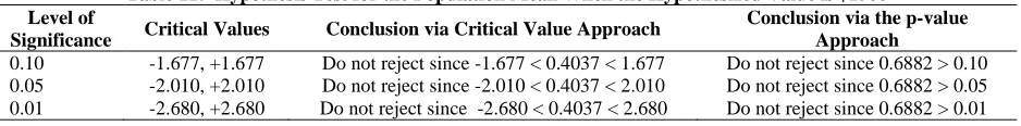
Students are then asked to pick a hypothesized value that they believe is the true population mean (e.g. $1500, $1525, $1550, etc.) and to run the hypothesis test again at levels of significance of 0.10, 0.05, and 0.01. If one selected a hypothesized value of $1500, then the null and alternative hypotheses are the following:

The test statistic is

and the p-value is 0.6882. Table 11 shows the conclusions to the hypothesis test for different levels of significance.

Table 11: Hypothesis Test for the Population Mean When the Hypothesized Value is $1500 Level of

Significance Critical Values Conclusion via Critical Value Approach

Conclusion via the p-value Approach

0.10 -1.677, +1.677 Do not reject since -1.677 < 0.4037 < 1.677 Do not reject since 0.6882 > 0.10 0.05 -2.010, +2.010 Do not reject since -2.010 < 0.4037 < 2.010 Do not reject since 0.6882 > 0.05 0.01 -2.680, +2.680 Do not reject since -2.680 < 0.4037 < 2.680 Do not reject since 0.6882 > 0.01

Confidence Intervals and Hypothesis Tests for the Population Proportion

Table 12: Confidence Intervals for the Population Proportion

Confidence Level z Value Lower Confidence Limit Upper Confidence Limit

90% 1.645 0.367 0.483

95% 1.960 0.356 0.494

99% 2.576 0.335 0.515

The null and alternative hypotheses when the hypothesized value is 0.50 are the following:

The following is the test statistic:

and the p-value is 0.034. Table 13 shows the conclusions of this hypothesis test for different levels of significance.

Table 13: Hypothesis Test for the Population Proportion When the Hypothesized Value is 0.50 Level of

Significance Critical Values Conclusion via Critical Value Approach

Conclusion via the p-value Approach 0.10 -1.645, 1.645 Reject since -2.12 < -1.645 Reject since 0.034 < 0.10 0.05 -1.960, +1.960 Reject since -2.12 < -1.960 Reject since 0.034 < 0.05 0.01 -2.576, +2.576 Do not reject since -2.576 < -2.12 < 2.576 Do not reject since 0.034 > 0.01

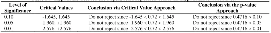
Students are then asked to pick a hypothesized value that they believe is the true population proportion of those who will definitely purchase breakfast items (Yes response). Students may pick values such as 0.40, 0.43, 0.45, etc. for the hypothesized value. If one selects 0.40 for the hypothesized value then the null and alternative hypotheses are as follows:

The following is the test statistic:

and the p-value is 0.4716. Table 14 shows the conclusions of this hypothesis test for different levels of significance.

Table 14: Hypothesis Test for the Population Proportion When the Hypothesized Value is 0.40 Level of

Significance Critical Values Conclusion via Critical Value Approach

Conclusion via the p-value Approach

AUTHOR INFORMATION