Vol. 05, Issue 05 (May. 2015), ||V2|| PP 01-08
Applicability of image processing for evaluation of surface
roughness
Omar Monir Koura
PhD, Lecturer in Mechanical Department, Faculty of Engineering, Modern University for Technology & Information, Egypt
Abstract: - Application of image processes is gaining greater potential nowadays particularly in automated manufacturing and in metrology world. It is a technique that has been claimed to be fast and reliable. One of the applications in engineering is the assessment of surface roughness. This application may be considered to be important as it deals with results their order of magnitude is the micron. Thus, in applying the technique of image processing to assess the surface roughness several parameters that is expected to affect the reliability and accuracy must be considered. This paper is not aimed at applying image processing to assess the surface roughness, but its main objective is to focus on the effects of some parameters such as the properties of the digital camera represented by its pixels, the relative setting of the camera with respect to the measured surfaces, the light intensity and the conditions of capturing the image such as shutter speed on the consistency of the results and to its reliability. The results show that the repeatability, reliability and accuracy of the resulted data depended to a great extent on such parameters. Variation of the results reached 33% in several cases. Artificial Neural Network was applied to determine the correlation between the results.
Keywords: - Image parameters, Image processing, Surface roughness, Gray scale, Artificial Neural Network.
I.
INTRODUCTION
Evaluation of surface quality is an essential aspect in part assembly and functioning performance. Traditionally, assessing surface roughness was performed by tracing the profile by a stylus technique /1/. However, such procedure was mainly, limited to 2D assessment. Automation in manufacturing and minimization of cost through reducing percentage of rejection has forced for high-speed, non-contact and reliable surface roughness assessment. Although many techniques were made available for surface roughness measurements, including the optical techniques, no technique has been established reliable and robust enough for the different applications. An optical technique through image processing is still faces several drawbacks due to the various parameters involved. Capturing an image from a camera requires a source of energy and a sensor array to sense the amount of light reflected by the object generating a continuous voltage signal by the amount of sensed data and converting this data into a digital form through sampling and quantization. Thus both the light intensity and type of the camera may be considered two parameters. Setting the camera (height of the camera and angle of the received rays) with respect to the object are further parameters that may affect the consistency of the results and their accuracies. A condition at which the image is taken such as speed of chatter is, again, a parameter.
Several researchers /2-6/ have used the image process to evaluate and predict the surface roughness parameters. However, they did not analyze or registered the conditions while taking and capturing the Images. On the other hand other researchers hinted about some factors affecting the captured images.
On the other hand, V. Elango & L. Karunamoorthy /7/ studied the lighting condition that affects the light scattering pattern of the surface and hence the image based optical surface finish parameter. The work was an attempt in the direction of evaluating the influence of lighting conditions on the optical surface finish parameter. They recorded great effects of the lighting situation such as the effect of the grazing angles and the ambient lighting variations.
Bernd Jähne and Horst Hauβecker /8/ analyzed in details several factors affecting the application of digital imaging systems to geometric calibration showing their importance.
T.Jeyapoovan and M.Murugan /9/ and Mindaugas Jurevicius, Jonas Skeivalas, Robertas Urbanavicius /10/ studied the classification of surface roughness using image processing. They hinted at some of the parameters affecting the images and carried out the work at specified values.
II.
PARAMETERS INVOLVED
Some factors affect the brightness and quality of the image such as aperture, shatter speed and shatter time which are directly affect the brightness of the captured image through controlling the amount of passed photons. Others may affect the resolution and accuracy of the achieved data particularly that in digital cameras, the image sensor senses the intensity of photon and convert it into digital information before storing the data and such sensors are manufactured by different companies with different techniques. Again, images are affected by the set up arrangement while taking the image. Distance of camera to specimen, normality of optical axis the surface to be tested may be, also, considered. Hence, the factors that will be considered in this paper are: - Height of the camera above the surface
- Angle setting of the camera to the normal of the tested surface - Illumination intensity
- Shatter speed
- Resolution of the digital camera
III.
EXPERIMENTAL PROCEDURE
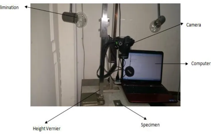
The test arrangement which is self explanatory is shown in fig 1. The test piece used is a standard reference specimen, its Ra value is 6.07 µm when measured at 2.5 mm cutoff, 2.5 mm sampling length and 12.5 mm evaluation length /1/.
Fig 1: Test arrangement
The captured images were taken by 3 different cameras (Nikon camera (Coolpix P510) 16.1 mega
pixels, Sony cyber shot 12.1 Mega pixels and Sony 9.1 Mega pixels) at shatter times range from 1
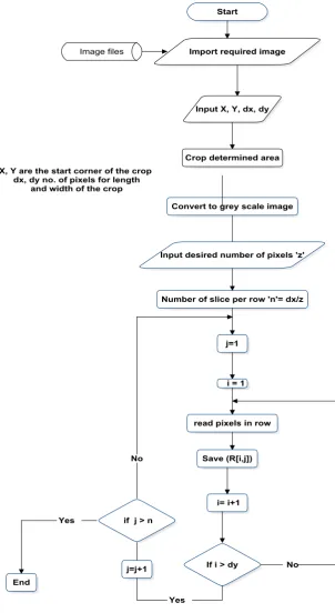
30 to 1 sec. at heights varied from 250 mm to 475mm. Camera was set at different inclination range from -12º to +12º . Captured images were analyzed using Matlab 2011. Fig 2 shows the block diagram of Gray Scale calculation. After selecting the captured image the start corner of the cropped area is selected. The number of the columns is fixed such that it is equivalent to the sampling length. The width of the cropped area is 5 times equivalent to the sampling length to represent the traverse length.
The gray index was calculated through counting the total gray heights (TGH) and getting the average (GHav = ƩTGH / n). n is the total number of the gray heights. The deviation of each gray height from the average was computed (∆GH = GH - GHav ). The Gray scale = Ʃ│∆GH│
Fig 2: Gray scale calculation
IV.
RESULTS
Effect of height
Fig 3: Effect of height on Gray scale
Effect of angle
Results for setting angle were taken by camera1 in ambient illumination. All results at different heights have shown a peak of gray scale when the camera was set with its optical axis as normal to the tested surface which indicate that light has reflected from greater numbers of peaks and valleys of the surface roughness.
Fig 4: Effect of angle on Gray scale
Effect of illumination intensity
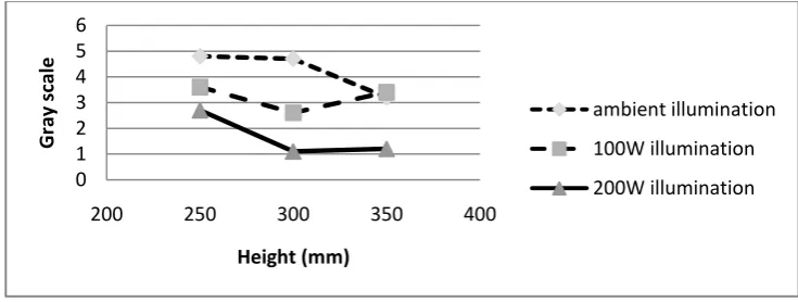
Fig 5 shows the results obtained when ordinary surrounding illumination is used and when two different light powers are used; namely 100 W and 200 W. The gray scale computed for the captured images at different heights were not consistent as the light intensity changed.
Fig 5: Effect of illumination on Gray scale 0 1 2 3 4 5 6 7 8 9
250 300 350
Gr ay scale Height (mm) camera 1 camera 2 camera 3 0 2 4 6 8 10 12
-20 -10 0 10 20
300 mm 250 mm 350 mm 0 1 2 3 4 5 6
200 250 300 350 400
The rapid decrease in the gray scale as the camera went behind 300 mm height when no other source of light was used could be attributed to the fact that the light falling on the specimen surface scatters differently with surface roughness and, hence, it is totally not recommended to use the uncontrolled light particularly at higher heights. Results with direct illumination proved to be better, but still an order of 50% variation was recorded as the intensity increased from 100W to 200W.
Effect of shatter speed
The effect of the shutter speed on the gray index, fig 6, indicates that the more time taken by the shatter the greater the representation of the gray height taken at the deeper valleys. Results with the camera set at lower height needs greater time. Again, variation of the resilts lie within 40%.
Fig 6: Effect of shatter speed on Gray scale
Effect of camera pixels
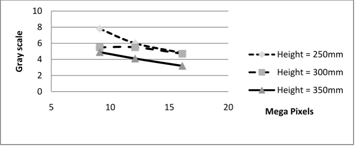
As the resolution of the camera increases, fig 7, less deviation of the gray heights resulted. Variations between different resolutions are limited to within 25%.
Fig 7: Effect of Camera pixels on Gray scale
Correlation of the results
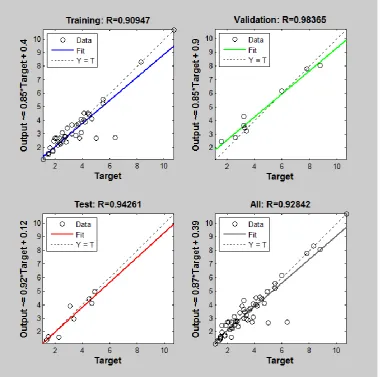
Artificial Neural Network (ANN) is applied to determine the correlation between the results. After several trials using the neural toolbox of Matlab 2011, the optimal structure was determined. It has 3 layers the first layer is consists of 5 neurons for the 5 inputs of the network (camera resolution, illumination intensity, camera height, shutter speed, and camera angle), the second layer is the hidden layer and it consist of 5 neurons, and the third layer is the output layer and it consists of 1 neuron.
The processing function for the hidden layer is logsig, and for the output layer is tansig. Feed-forward back propagation ANN used, Leven berg-Marquardt back propagation (TRAINLM) algorithm is used for network training and mean square error (MSE) is used as performance function.
0 2 4 6 8 10
0 1/5 2/5 3/5 4/5 1 1 1/5
300 mm
350 mm
0 2 4 6 8 10
5 10 15 20
Gr
ay
scale
Mega Pixels
Height = 250mm
Height = 300mm
Fig 8: Neural structure
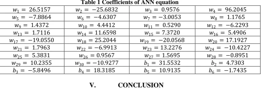
The results show that the correlation coefficient between the measured values and predicted values is 0.92842, as shown in fig 9. The equations that provide the corrected gray scale for the combined parameters are given below. Table 1 gives the values of the coefficients.
Gray scale = (253.8*H1) +255.2 Where:
𝐻1=
2
1+ 𝑒−2(𝑤 26 ℎ1+ 𝑤 27 ℎ2+ 𝑤 28 ℎ3+ 𝑤 29ℎ 4+𝑤 30ℎ 5+𝑏6)
h1=
1
1+ e−(w 1y 1+ w 2y 2+ w 3y 3+ w 4y 4+w 5y 5+b 1)
h2=
1
1+ e−(w 6y 1+ w 7y2+ w 8y 3+ w 9y 4+w 10 y 5+b 2)
h3=
1
1+ e−(w 11 y 1+ w 12 y 2+ w 13 y3+ w 14 y4+w 15 y 5+b 3)
h4=
1
1+ e−(w 16 y 1+ w 17 y 2+ w 18 y3+ w 19 y4+w 20 y 5+b 4)
h5=
1
1+ e−(w 21 y 1+ w 22 y 2+ w 23 y3+ w 24 y4+w 25 y 5+b 5)
𝑦1= (0.285 * R) - 3.6
𝑦2= (0.01 * I) - 1.105
𝑦3= (0.008 * h) - 3.222
𝑦4= (2.068 * s) - 1.068
𝑦5= (0.083 * a)
R is the camera pixels (megapixels), I is the intensity (Watt), h is the camera height (mm), s is the chatter speed (sec.) and a is the inclination (deg.).
Table 1 Coefficients of ANN equation
𝑤1= 26.5157 𝑤2= −25.6832 𝑤3= 0.9576 𝑤4= 96.2045
𝑤5= −7.8864 𝑤6= −4.6307 𝑤7= −3.0053 𝑤8= 1.1765
𝑤9= 1.4372 𝑤10= 4.4412 𝑤11= 0.5290 𝑤12= −6.2293
𝑤13= 1.7116 𝑤14= 11.6598 𝑤15= 7.3720 𝑤16= 5.4906
𝑤17= −19.0550 𝑤18= 25.2044 𝑤19= −20.0568 𝑤20= 17.1927
𝑤21= 1.7963 𝑤22= −6.9913 𝑤23= 13.2276 𝑤24= −10.4227
𝑤25= 5.3831 𝑤26= 0.9567 𝑤27= 1.5695 𝑤28= −0.8951
𝑤29= 10.2355 𝑤30= −10.9277 𝑏1= 31.5532 𝑏2= 4.7303
𝑏3= −5.8496 𝑏4= 18.3185 𝑏5= 10.9135 𝑏6= −1.7435
V.
CONCLUSION
Applying image processing to accurate fields such as assessment of surface roughness need to be carefully dealt with. Without considering the setting of the camera with respect to the part to be measured and the conditions of taking the images affect to great extent the consistency of the results. Variation exceeded 33%. Camera resolution has little effect within the range considered (9.1 to 16.1 Megapixels). Perpendicularity of the optical axis of the camera to the surface is a must. Artificial Neural Network showed correlation between the different parameters and the gray scale to be within 0.9284 and presented the equations that should be used to calculate the correct gray scale.
VI.
ACKNOWLEDGEMENT
The author wishes to express his thanks to Eng. A. S. AlAkkad (Researcher in Design and Production Dept., Faculty of Eng., Ain Shams University) for his great assistant in carrying out the experimental work.
REFERENCES
[1]. http://www.surfaceroughnesstester.com/surfaceroughnessparameters.html.
[2]. B. Dhanasekar, N. Krishna Mohan, Basanta Bhaduri, B. Ramamoorthy, “Evaluation of surface roughness based on monochromatic speckle correlation using image processing”, Precision Engineering, V32, 2008, pp 196 – 206
[3]. S. Palani & U. Natarajan, “Prediction of surface roughness in CNC end milling by machine vision system using artificial neural network based on 2D Fourier transform”, International Journal of advanced technology, 2011, 54, pp1033-1042
[4]. Mohan Kumar Balasundaram and Mani Maran Ratnam, “In-Process Measurement of Surface Roughness using Machine Vision with Sub-Pixel Edge Detection in Finish Turning”, International Journal of Precision Engineering and Manufacturing Vol 15, No. 11, pp2239-2249
362
[6]. S. H. Yang & U. Natarajan & M. Sekar & S. Palani, “ Prediction of surface roughness in turning operations by computer vision using neural network trained by differential evolution algorithm”, International Journal of advanced technology, 2010, 51, pp965-971
[7]. H. H. Shahabi & M. M. Ratnam, “ Prediction of surface roughness and dimensional deviation of workpiece in turning: a machine vision approach”, International Journal of advanced technology, 2010, 48, pp213-226 [8]. V. Elango & L. Karunamoorthy, “Effect of lighting conditions in the study of surface roughness by machine
vision - an experimental design approach, International Journal of advanced technology, 2008, 37, pp92-103. [9]. Computer vision and applications, “ Bernd Jähne and Horst Hauβecker, Publisher - Academic Press, 2000 [10]. T. Jeyapoovan, M. Murugan, “Surface roughness classification using image processing”, Measurement, V46,
2013, pp 2065 - 2072
[11]. Mindaugas Jurevicius, Jonas Skeivalas, Robertas Urbanavicius, “Analysis of surface roughness