www.nonlin-processes-geophys.net/23/75/2016/ doi:10.5194/npg-23-75-2016
© Author(s) 2016. CC Attribution 3.0 License.
Study of the overturning length scales at the Spanish
planetary boundary layer
Pilar López1and José L. Cano2
1Applied Mathematics Dpt. (Biomathematics), Complutense University of Madrid, Madrid, Spain
2Astronomy, Astrophysical and Atmospheric Science Dpt., Complutense University of Madrid, Madrid, Spain
Correspondence to: Pilar López ([email protected])
Received: 28 September 2015 – Published in Nonlin. Processes Geophys. Discuss.: 20 November 2015 Revised: 12 February 2016 – Accepted: 23 February 2016 – Published: 21 March 2016
Abstract. The focus of this paper is to analyse the be-haviour of the maximum Thorpe displacement (dT)maxand
the Thorpe scale LT at the atmospheric boundary layer
(ABL), extending previous research with new data and im-proving our studies related to the novel use of the Thorpe method applied to ABL. The maximum Thorpe displace-ments vary between−900 and 950 m for the different field campaigns. The Thorpe scale LT ranges between 0.2 and
680 m for the different data sets which cover different strati-fied mixing conditions (turbulence shear-driven and convec-tive regions). We analyse the relationship between (dT)max
and the Thorpe scale LT and we deduce that they verify a
power law. We also deduce that there is a difference in expo-nents of the power laws for convective conditions and shear-driven conditions. These different power laws could identify overturns created under different mechanisms.
1 Introduction
The atmospheric boundary layer (or ABL) is almost always turbulent. In the absence of turbulence, atmospheric tem-perature profiles become increasingly monotonic, due to the smoothing effect of molecular diffusion. Turbulence gives rise to an effective eddy diffusivity and together with other causes (such as fluid instabilities or internal wave breaking) makes vertical overturns appear as inversions in measured temperature profiles. These overturns produce small-scale turbulent mixing which is of great relevance for many pro-cesses ranging from medium to local scales. Unfortunately, measuring at small scales is very difficult. To overcome this disadvantage it is interesting to use theories and
parameter-izations which are based on larger scales, for example, the theories of turbulent stirring which often depend on hypothe-ses about the length scales of turbulent eddies. Vertical over-turns, produced by turbulence in density stratified fluids such as lakes or the ABL, can often be quantified by the Thorpe displacementsdTand the Thorpe scaleLT(Thorpe, 1977).
Next we present the atmospheric data used for the analysis. In Sect. 3 we present the Thorpe method and the definitions of the scale descriptors used. In Sect. 4, the results of Thorpe displacements, the maximum Thorpe displacement, and the Thorpe scaleLTat the ABL are presented and discussed.
2 Atmospheric data sets and meteorological instrumentation
At-time. A detailed description can be consulted in Cuxart et al. (2000). The Sables98 field campaign only collects data over the night and, therefore, under neutral to stable con-ditions. The Sables2006 field campaign took place from 19 June to 5 July 2006 at the CIBA. As in Sables98, different instrumentation was available on a tower of 100 m; a sur-face triangular array of microbarometers was also deployed and a tethered balloon was used to get vertical profiles up to 1000 m. As in Sables98, the Sables2006 field campaign also collects data over the night. Therefore, the Sables98 and Sables2006 experiments let us analyse the behaviour of over-turns under stable conditions, while Almaraz94-95 is under unstable conditions (and also stable ones). These three sets of data were selected for this analysis because they cover differ-ent mixing conditions (turbulence shear-driven and convec-tive regions).
3 Thorpe method and overturn length scales
Thorpe devised an objective technique for evaluating a ver-tical length scale associated with overturns in a stratified flow (Thorpe, 1977; Itsweire, 1984; Gavrilov et al., 2005). Thorpe’s technique consists of rearranging a density profile (which contains gravitationally unstable inversions) so that each fluid particle is statically stable. If the sample at depth znmust be moved to depthzmto generate the stable profile, the Thorpe displacementdTiszm−zn(Thorpe, 1977; López
et al., 2008, 2016). The Thorpe displacementdTis not
nec-essarily the real space actually travelled by the fluid sample. It is an estimate of the vertical distance from the given verti-cal profile to the stativerti-cally stable one that each fluid particle has to move upward or downward to its position in the stable monotonic profile (Thorpe, 1977; Dillon, 1982). Over most of a typical profile, the local stratification will be stable and the Thorpe displacement zero. A turbulent event is, therefore, defined as a region of continuously nonzerodT, that is,
over-turns are defined as a profile section for which P i
dTi=0, whiledTi6=0 for mosti(Dillon, 1982; Peters et al., 1995).
The maximum of the Thorpe displacement scale (dT)max=max [dT(z)] represents the larger overturns which
might have occurred at earlier times when buoyancy effects were negligible (Thorpe, 1977; Dillon, 1982; Itsweire, 1984), and it could be considered an appropriate measure of the overturning scale.
The Thorpe scale LT is the root mean square (rms) of
the Thorpe displacements(LT)rms=LT=
dT2(z)1/2. There-fore, it is a statistical measure of the vertical size of overturn-ing eddies (Thorpe, 1977; Dillon, 1982; Itsweire, 1984; Fer
dient (4×10⁻⁴(K m−1)) is smaller than the average vertical temperature gradient (2×10⁻²(K m−1)) (López et al., 2016). Because of the expensive nature of collecting data at mi-croscale resolution, there is a great interest in using param-eterizations for small-scale dynamics which are based on larger scales – as LT or (dT)max. Therefore, it is very
im-portant to analyse the relationship betweenLTand(dT)max
for selecting the most appropriate overturning scale.
4 Quantitative results
Our methodology is based on reordering 111 measured po-tential temperature profiles, which may contain inversions, to the corresponding stable monotonic profiles. Then, the vertical profiles of the displacement length scalesdT(z) or
Thorpe displacement profiles can be calculated by using a bubble sort algorithm with ordering beginning at the shallow-est depth (Thorpe, 1977; Dillon, 1982; Itsweire, 1984; López et al., 2008, 2016). This simple sorting algorithm works by repeatedly stepping through the data list to be sorted, com-paring each pair of adjacent items, and swapping them if they are in the wrong order (López et al., 2016).
4.1 Thorpe displacement profiles at ABL
Figure 1. Left curve: Thorpe displacementDth profile with an iso-lated patch corresponding to 07:00 GMT. Right curve: Thorpe dis-placement Dth profile with a random mix of fluctuations corre-sponding to 17:00 GMT.
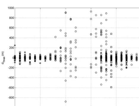
Figure 2. Time evolution of the maximum Thorpe displacements during a day cycle. The symbols are as follows:◦is for Almaraz94-95 data,?is for Sables98 data, andis for Sables2006 data. The error of Thorpe displacements is±1 m.
under convective and/or neutral conditions (at noon, after-noon, and evening profiles). These Thorpe displacements are rarely zero for the whole profile. To verify this behaviour, see López et al. (2008) and López et al. (2016).
4.2 Time evolution of maximum Thorpe displacements and Thorpe scales
Figure 2 shows the time evolution of the maximum Thorpe displacement (dT)max along a day for the three field
cam-paigns. The scale(dT)maxis very small (approximately zero)
under stable conditions from 23:00 to 06:00 GMT (between
Figure 3. Time evolution of the Thorpe scale during a day cycle. The symbols are as follows:◦is for Almaraz94-95 data,? is for Sables98 data, andis for Sables2006 data. The error of Thorpe displacements is±1 m.
sunset and sunrise) for all the experiments. From 19:00 GMT, it is observed that scale (dT)max decreases. The greatest
values of(dT)maxappear under convective conditions from
09:00 to 19:00 GMT that are positive and negative. But the positive values of(dT)maxare greater than the negative ones.
The positive (dT)max has its greatest values about 950 m
and the greatest negative (dT)max is about 600 m
(abso-lute value). These results mean the following. Thorpe dis-placements were defined as the difference between the fi-nal height and the initial height of the fluid particle, i.e. dT=(zm)final−(zn)initial. If dT>0((zm)final>(zn)initial), the
fluid particle has to go up to reach its stable position, and ifdT<0 ((zm)final<(zn)initial), it has to go down to reach its
stable point. From Fig. 2 we can deduce that fluid particles go upwards and downwards with a greater vertical distance under convective stratification conditions. Under stable strat-ification conditions – at night –, the fluid particles also move upwards and downwards, but with small values for the ver-tical distance travelled. Hence, it is clear that the maximum Thorpe displacement is always greater under convective con-ditions than under stable ones, independent of its sign. There-fore, the maximum Thorpe displacements are a parameter which could represent the dynamical behaviour of air par-ticles and its relationship with the stratification conditions. Finally, there is a gap in Fig. 2 due to unregistered data be-tween 13:00 and 14:00 GMT.
Figure 3 shows the time evolution of the Thorpe scale, LT, during a day for the three field campaigns. The Thorpe
scaleLThas small values (close to zero) under neutral and
conditions, Thorpe scales are relatively large. They exceed hundreds of metres and they may be related to convective bursts. Hence, the Thorpe scaleLTis always greater under
convective conditions than under stable ones, and it is a pa-rameter which could also represent the dynamical behaviour of air particles. As in Fig. 2, there is a gap in Fig. 3 due to the unregistered data between 13:00 and 14:00 GMT. Both scales, the Thorpe scale LT and the maximum Thorpe
dis-placement (dT)max, have small values (close to zero) under
neutral and stable conditions, and their greatest values ap-pear under convective conditions. Therefore, it is reasonable to think about which of the two scales could represent better the dynamical behaviour of turbulent overturns.
Moreover, it is necessary to choose an appropriate over-turning scale to characterize instabilities leading to turbu-lent mixing and the turbuturbu-lent overturning motions them-selves, and to look for a relationship with the Ozmidov scale at ABL data (Dillon, 1982; Lorke and Wüest, 2002; Fer et al., 2004). We could choose the Thorpe scale rather than the maximum Thorpe displacement because we only sample vertically, while the turbulence is three dimensional and, therefore, the Thorpe scale is more likely to be a sta-tistically stable representation of the entire feature (Dillon, 1982). But the maximum of the Thorpe displacements is also considered to be an appropriate measure of the overturning scale and it is always greater thanLT (better detectable by
a limited-resolution instrument). Different researchers have found a linear model between LT and(dT)max for profiles
from the equatorial undercurrent (Moum, 1996; Peters et al., 1995) and a high linear correlation computed from the Banyoles99 field data where the ratio(dT)max/LTis
approx-imately equal to 3 (Piera, 2004). A correlation must exist be-tweenLT and(dT)maxbecause when computing the rms of
a set of Thorpe displacements with high kurtosis distribu-tions, the final result depends on the largest values (Piera, 2004; Stansfield et al., 2001). A similar linear correlation be-tweenLTand(dT)maxhas been found by other researchers:
a ratio(dT)max/LT≈3.3 is obtained in the oceanic
thermo-cline (Moum, 1996), a ratio (dT)max/LT≈2.4 is obtained
from laboratory experiments (Itsweire et al., 1993) and, fi-nally, the ratio (dT)max/LT is nearly 3 in numerical
sim-ulations (Smyth and Moum, 2000). But for microstructure profiles from strongly stratified lakes, a power law – such as (dT)max∼(LT)0.85 – is found (Lorke and Wüest, 2002).
This relation also holds for profiles from other lakes under very different conditions of mixing and stratification, with a strong correlation that holds over 4 orders of magnitude (Lorke and Wüest, 2002).
Hence, we analyse the relation between the LT and
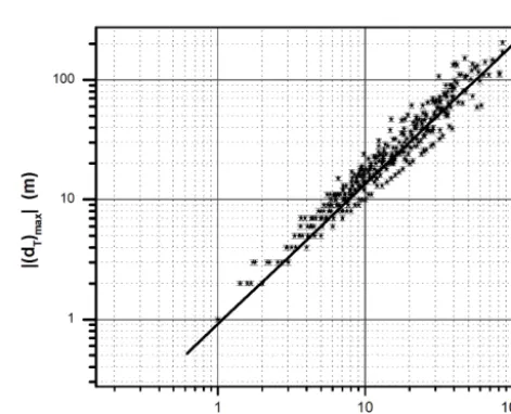
(dT)maxscales for our ABL data. Figure 4 shows the
max-Figure 4. Absolute value of the maximum Thorpe displacement versus the Thorpe scale. The symbols are as follows: ◦ is for Almaraz94-95 data,?is for Sables98 data, andis for Sables2006 data.
imum Thorpe displacement versus the Thorpe scale at a log scale, using the data of the three field campaigns. We observe that the linear model proposed by other authors (Moum, 1996; Peters et al., 1995; Piera, 2004; Itsweire et al., 1993; Smyth and Moum, 2000) does not agree with our ABL data. Therefore, we could think that the nearly constant ratio (dT)max/LT obtained in a wide range of field and
labora-tory experiments is not verified in our ABL data (Fig. 4). And, hence, the shape of the Thorpe displacement distribu-tion could change at the ABL. We also observe a strong cor-relation which holds over 3 orders of magnitude as in other studies from profiles in lakes (Lorke and Wüest, 2002). It is the first time that such a relationship between these two over-turning length scales is found for ABL data (Fig. 4).
Like other authors, we could state that this high correlation indicates that the Thorpe scale is determined by the overturns near to the maximum Thorpe displacement. We find the fol-lowing power law:
(dT)max
∼(LT)1.14, (1)
which is similar to the one deduced by Lorke (Lorke and Wüest, 2002) from profiles in strongly stratified lakes. We perform a simple linear regression analysis. Of particular in-terest is the p value1 associated with the analysis of
ance2, which tests the statistical significance of the fitted model. For our case the p value is less than 0.05 (operat-ing at the 95 % confidence level), which indicates that the linear model between |(dT)max| and LT is statistically
sig-nificant. Moreover, theR2coefficient3is 96.95 %, which in-dicates that the linear simple regression accounts for about 97 % of the variability in the maximum Thorpe displacement
|(dT)max|as a function of the Thorpe scale,LT, statistically.
This relation between the maximum Thorpe displacement and the Thorpe scale by a power law has been deduced for the overall data (not separating the data from the three field campaigns). But we have used a data set with three dif-ferent experiments under difdif-ferent mixing conditions. The SABLES98 and SABLES2006 experiments were conducted at night (turbulence by shear-driven) and ALMARAZ94-95 during a day cycle and, therefore, convective regions have not been excluded. Hence, we consider analysing whether this power law is different from night to day. The objec-tive is to study whether it is possible to distinguish between the shear-driven overturns and the convective ones. First, we separate the data from the three experiments into two sets: data obtained overnight (from the Sables98, Sables2006, and Almaraz94-95 field campaigns), or the night data set, and data which have been obtained during the day (only from the Almaraz experiment), or the day data set. Then we perform a linear simple regression analysis with an adjustment by least squares for the two data sets. And, finally, we make a com-parison of the regression lines relating |(dT)max|andLT at
the two levels of our categorical factor (daytime and night-time).
Figure 5 represents the maximum Thorpe displacement versus the Thorpe scale only for the daytime data set (from 07:00 to 19:00 GMT). We observe a strong correlation which holds over 3 orders of magnitude as was deduced for the whole data set and other studies (Lorke and Wüest, 2002).
We perform the linear simple regression analysis. The p value associated with the analysis of variance is less than 0.05 (operating at the 95 % confidence level4), which indi-cates that the linear fit between |(dT)max|andLT is
statis-tically significant as before. The R2 coefficient represents
2The analysis of variance (ANOVA) is a statistical tool that sep-arates the total variability of a data set into two components: ran-dom (which do not have any statistical influence on the given data set) and systematic factors (which have some statistical effect on the data). The ANOVA test is used to determine the impact independent variables have on the dependent variable in a regression analysis.
3TheR2coefficient is called the determination coefficient which represents the proportion of the variance (fluctuation) of one vari-able that is predictvari-able from the other varivari-able. It is a measure that allows us to determine how certain one can be in making predictions from a certain model. In our case, the coefficient of determination is a measure of how well the regression line represents the data.
4The confidence level is a measure of the reliability of a result. A confidence level of 95 % or 0.95 means that there is a probability of at least 95 % that the result is reliable.
Figure 5. Absolute value of the maximum Thorpe displacement versus the Thorpe scale for the daytime data set (N). The linear fit is indicated by the continuous black line.
Figure 6. Absolute value of the maximum Thorpe displacement versus the Thorpe scale for the nighttime data set (◦). The linear fit is indicated by the continuous black line.
the percentage of the variability in|(dT)max|, which has been
explained by the fitted linear regression model and is about 97 %.
Figure 6 represents the maximum Thorpe displacement versus the Thorpe scale only for the nocturnal data set (from 20:00 to 06:00 GMT). We also observe a strong correlation which holds over 3 orders of magnitude as before (see Figs. 4 and 5).
be-scaleLT by a power law is different from day to night. For
the nighttime data set, the power law is
(dT)max
∼(LT)1.17. (2)
And for the daytime data set, the relation is the following:
(dT)max
∼(LT)1.12. (3)
We observe that the kind of relation is the same (a power law) but the exponents are different. So we question whether these coefficients are statistically different and whether there is or is not a different behaviour of the overturn length scales between day and night.
These exponents are the slopes of the regression lines fit-ted to daytime and nighttime data sets (see Figs. 5 and 6). To know whether they are statistically different, we need to perform a comparison of regression lines. This procedure is a test to determine whether there are significant differences between the intercepts and the slopes at the different levels of our factor (day and night). This test fits two different re-gression lines to the nighttime and daytime data sets and per-forms two analyses of variance (one for each linear model and secondly for comparing the two regression lines). For the first analysis, the p value is less than 0.05, if we oper-ate at the 5 % significance level, and indicoper-ates that the linear fit between |(dT)max| and LT is statistically significant for
daytime and nighttime data sets (t-statistic tests5 have also been performed whose pvalues are less than 0.05, indicat-ing that the model coefficients are significantly different from 0). The second analysis of variance is performed to deter-mine whether there are significant differences between the slopes of the daytime and nighttime fitted lines. TheF test6 for slopes tests whether the slopes of the lines are all equal. Operating at the 1 % significance level7, we find ap value (for slopes) which is less than 0.01, and, therefore, there are significant differences between the slopes of the daytime and nighttime lines (we get the same result for the intercepts).
There is one more question, that is, to analyse whether the power law fits the data better than a linear one in sta-tistical terms. We have made a simple regression analysis to
5A two-samplettest examines whether two samples are differ-ent, and it is a statistical analysis of two population means.
6TheFtest tests the statistical significance of the fitted model. A smallpvalue (less than 0.05) indicates that a significant relation-ship of the form specified exists between two variables,y andx. It is most often used when comparing statistical models that have been fitted to a data set, in order to identify the model that fits best. 7In hypothesis testing, the significance level is the criterion used for rejecting the null hypothesis (a hypothesis about a popula-tion parameter). The significance level is the probability of rejecting the null hypothesis given that it is true.
significance of the fitted model.
For all three data sets, we got the same results. The analysis of variance indicated that a linear model between
|(dT)max| and LT is statistically significant (because the
pvalue is less than 0.05). But theR2– or determination co-efficient – which represents the percentage of the variability in|(dT)max|which has been explained by the fitted regression
model is less in the power law fit (87.9 % for the whole data set, 84 % for the daytime data set, and 90.11 % for the night-time data set) than in the linear one (96.95 % for the whole data set, 96.76 % for the daytime data set, and 95.89 % for the nighttime data set). As a consequence, the remainder of the unexplained variability is attributable to deviations around the line, which may be due to other factors, for example, to a failure of the linear model to fit the data adequately. We con-clude that both models, the power law fit and the linear one, are statistically significant, but the power law fit has a bet-ter debet-termination coefficient and accounts betbet-ter for the vari-ability in the maximum Thorpe displacement measurements. Therefore, we consider the power law fit to be the best fitted model for the three data sets.
Finally, we deduce that the two power relations between the maximum Thorpe displacement|(dT)max|and the Thorpe
scaleLTfor nighttime data (Eq. 2) and daytime data (Eq. 3)
are significant different, with a 99 % confidence level. There-fore, we could classify overturns as day and night ones; that is, we could distinguish between convective and shear-driven mechanism originating overturns.
As mentioned before, although both scales(dT)maxandLT
are alternative length scales to characterize turbulent over-turns, it is reasonable to choose one of the two scales to represent better overturns. If there is a high linear corre-lation between the maximum Thorpe displacement(dT)max
and the Thorpe scaleLT, the last one could be considered
a better descriptor of the overturn properties, although it de-pends mainly on the values of(dT)max, and the relative errors
from both scales are approximately equal (Piera, 2004). But we have just deduced that the relationship between the max-imum Thorpe displacement (dT)max and the Thorpe scale
LT does not follow a linear model in our ABL research,
unless as a power law as with other authors (Lorke and Wüest, 2002). Consequently, there would not be a constant ratio|(dT)max|/LT, which could suggest that the shape of the
Thorpe displacement distribution could change. Therefore, it is necessary to study the probability density functions (pdfs) of the Thorpe displacements to understand better the relation-ship between(dT)maxandLT. Moreover, the Thorpe scale is
of the Thorpe displacements. This pdf study would allow us to decide which of the two overturn length scales is a more representative measure of turbulent overturns.
5 Conclusions
The paper presents results related to the time evolutions of the ABL turbulent parametersLTand(dT)maxduring a day
with different levels of stability. Secondly, the paper adds in-sight into the problem of the relationship between these two overturning length scales at the ABL.
The Thorpe scaleLTand the maximum Thorpe
displace-ment (dT)max have small values under neutral and stable
conditions, and their greatest values appear under convec-tive conditions. The values of the Thorpe scale range in (1, 660) m, which are greater than effective values in the stratosphere which areLT∼1–1.1 m (Gavrilov et al., 2005),
values in mixing surface layers and seasonal thermoclines which are LT∼0.03–1.90 m (Dillon, 1982), values in the
vertical mixing process induced by internal tides which are LT∼0.2–4.2 m (Kitade et al., 2003), or values in dense
over-flow which areLT∼1–17 m (Fer et al., 2004). The greater
values appear under convective conditions which could gen-erate overturns of a larger scale. Under shear-driven condi-tions, our Thorpe scales are smaller than convective ones, ranging in (1, 100) m, but they are also greater if we com-pare them with the scales of other authors. Therefore, we deduce that there would be a relationship between the ABL processes which generate mixing and the overturn size and behaviour (for example, the terrain shape interacts with the ability of the ABL to produce local mixing very near the ground, and this could be affect overturns). This theme will need further field work where different conditions are met (combination of the boundary condition effects and of sta-bility combining the 3-D and 2-D characteristics of scale-to-scale direct and inverse cascades, intermittency of the forc-ing, and scale-to-scale stratified turbulence cascades (Vindel et al., 2008; Yagüe et al., 2006)).
Equations (1) to (3) show that the relationship between the Thorpe scaleLT, and the maximum Thorpe displacement
(dT)maxis a power law which has been statistically
demon-strated. We must therefore conclude that the linear model proposed by other authors (Moum, 1996; Peters et al., 1995; Piera, 2004; Itsweire et al., 1993; Smyth and Moum, 2000) is not adequate for our ABL data. Research will continue on this interesting question which is related to the selection of a length scale for characterizing turbulent overturns. This last problem would be better analysed if we were to study the probability density function (pdf) of overturning length scales. The objective is to decide whether LT is or is not
statistically a more appropriate length scale than (dT)max.
Moreover, it is interesting to verify the assumption that the Thorpe scales have a universal probability density function which could be used to verify how accurately the Thorpe
scales were computed and also to determine whether(dT)max
is statistically better thanLTas an overturning length scale.
It is very likely that the pdf parameters depend on the govern-ing background conditions generatgovern-ing Thorpe displacements, which are different in the boundary layers from those in the interior layers with intermittent mixing, or in convective con-ditions from shear-driven concon-ditions. We also would like to verify whether the density probability function is decaying exponentially for increasing displacement length with a sep-arate cut-off before(dT)max.
In the future, we will go on studying the power relationship between the maximum Thorpe displacement and the Thorpe scale corresponding to ABL data to verify the power law de-duced in this paper. For this purpose, we will use a new set of ABL data from new field campaigns. We will analyse the probability density function of overturning length scales to clarify better the relation between(dT)maxandLT and as a
tool to choose the more appropriate turbulent patch length scale. Moreover, we would like to study the following hy-pothesis that if the Thorpe scale is greater than the integral scale, there would be a local convective process and, if it is not, there would be stratification.
Finally, there is another subject which is important to men-tion. In future research, we need to study better the over-turn identification as in Piera et al. (2002). They propose a new method based on wavelet denoising and the analysis of Thorpe displacement profiles for turbulent patch identifi-cation. Although their method is for microstructure profiles (which is not our case), it reduces most of the noise present in the measured profiles (increasing the resolution of the over-turn identification) and is very efficient even at very low-density gradients for turbulent patch identification. Another way to get overturn identification would be, for example, to use a 3- or 4-D parameter space formed by (LO, LT, LMO)
to locate mixing events and also to study the evolution of the processes.
Acknowledgements. In memory of my mother, Elena.
This work was financially supported by the Spanish Ministry of Education and Science (projects CGL2009-12797-C03-03 and CGL2012-37416-C04-02), which is gratefully acknowledged. We are also in debt to all the team participating in ALMARAZ94-95, SABLES98 and SABLES2006. The authors also acknowledge the help of ERCOFTAC (SIG 14). We acknowledge the referees for assisting in evaluating this paper; their constructive criticism helped in improving the manuscript.
Edited by: P. Fraunie
References
Fer, I., Skogseth, R. and Haugan, P. M.: Mixing of the Storfjor-den overflow (Svalbard Archipelago) inferred from Storfjor-density over-turns, J. Geophys. Res., 109, 1–14, doi:10.1029/2003JC001968, 2004.
Gavrilov, N. M., Luce, H., Crochet, M., Dalaudier, F., and Fukao, S.: Turbulence parameter estimations from high-resolution bal-loon temperature measurements of the MUTSI-2000 campaign, Ann. Geophys., 23, 2401–2413, doi:10.5194/angeo-23-2401-2005, 2005.
Itsweire, E. C.: Measurements of vertical overturns in stably strati-fied turbulent flow, Phys. Fluids, 27, 764–766, 1984.
Itsweire, E. C., Kossef, J. R., Briggs, D. A., and Ferziger, J. H.: Turbulence in stratified shear flows: Implications for interpreting shear-induced mixing in the ocean, J. Phys. Oceanogr., 23, 1508– 1522, 1993.
Kitade, Y., Matsuyama, M., and Yoshida, J.: Distribution of overturn induced by internal tides and Thorpe scale in Uchiura Bay, J. Oceanogr., 59, 845–850, 2003.
López, P., Cano, J. L., Cano, D., and Tijera, M.: Thorpe method applied to planetary boundary layer data, Il Nuovo Cimento, 31C, 881–892, doi:10.1393/ncc/i2009-10338-3, 2008.
López, P., Redondo, J. M., and Cano, J. L.: Thorpe scale at the planetary boundary layer: Comparison of Almaraz95 and Sables98 experiments, Complex Environmental Turbulence and Bio-Fluids Flows, Institute of Thermomechanics AS CR, Prague, in press, 2016.
Peters, H., Gregg, M. C., and Sanford, T. B.: Detail and scaling of turbulent overturns in the Pacific equatorial undercurrent, J. Geophys. Res., 100, 18349–18368, 1995.
Piera, J.: Signal processing of microstructure profiles: integrating turbulent spatial scales in aquatic ecological modelling, PhD Thesis, Gerona University, Spain, 2004.
Piera, J., Roget, E., and Catalan, J.: Turbulent patch identification in microstructure profiles: a method based on wavelet denoising and Thorpe displacement analysis, J. Atmos. Ocean. Tech., 19, 1390–1402, 2002.
Smyth, W. D. and Moum, J. N.: Length scales of turbulence in sta-bly stratified mixing layers, Phys. Fluids, 12, 1327–1342, 2000. Stansfield, K., Garret, C., and Dewey, R.: The probability
distri-bution of the Thorpe displacements within overturns in Juan de Fuca Strait, J. Phys. Oceanogr., 31, 3421–3434, 2001.
Thorpe, S. A.: Turbulence and Mixing in a Scottish Loch, Philos. Trans. R. Soc. London A, 286, 125–181, 1977.
Vindel, J. M., Yagüe, C., and Redondo, J. M.: Structure function analysis and intermittency in the atmospheric boundary layer, Nonlin. Processes Geophys., 15, 915–929, doi:10.5194/npg-15-915-2008, 2008.