1Nansen Environmental and Remote Sensing Center, Thormohlensgate 47, Bergen, 5009, Norway 2Institute for Space Research and Technology, Technical University of Denmark, Lyngby, Denmark
3Department of Space, Earth and Environment, Microwave and Optical Remote Sensing, Chalmers University of Technology, Gothenburg, Sweden
4Institute of Environmental Physics, University of Bremen, Bremen, Germany
5Department of Remote Sensing And Data Management, Norwegian Meteorological Institute, Oslo, Norway 6Department of Remote Sensing And Data Management, Norwegian Meteorological Institute, Tromsø, Norway
7Ifremer, Univ. Brest, CNRS, IRD, Laboratoire d’Oceanographie Physique et Spatiale (LOPS), IUEM, 29280, Brest, France Correspondence:Anton Andreevich Korosov ([email protected])
Received: 4 November 2017 – Discussion started: 15 November 2017 Revised: 22 May 2018 – Accepted: 25 May 2018 – Published: 15 June 2018
Abstract.A new algorithm for estimating sea ice age (SIA) distribution based on the Eulerian advection scheme is pre-sented. The advection scheme accounts for the observed di-vergence or condi-vergence and freezing or melting of sea ice and predicts consequent generation or loss of new ice. The al-gorithm uses daily gridded sea ice drift and sea ice concentra-tion products from the Ocean and Sea Ice Satellite Applica-tion Facility. The major advantage of the new algorithm is the ability to generate individual ice age fractions in each pixel of the output product or, in other words, to provide a frequency distribution of the ice age allowing to apply mean, median, weighted average or other statistical measures. Comparison with the National Snow and Ice Data Center SIA product re-vealed several improvements of the new SIA maps and time series. First, the application of the Eulerian scheme provides smooth distribution of the ice age parameters and prevents product undersampling which may occur when a Lagrangian tracking approach is used. Second, utilization of the new sea ice drift product void of artifacts from EUMETSAT OSI SAF resulted in more accurate and reliable spatial distribution of ice age fractions. Third, constraining SIA computations by the observed sea ice concentration expectedly led to con-siderable reduction of multi-year ice (MYI) fractions. MYI concentration is computed as a sum of all MYI fractions and compares well to the MYI products based on passive and ac-tive microwave and SAR products.
1 Introduction
Sea ice age (SIA) is one of the components of the essential climate variable (ECV) for sea ice as defined by the Global Climate Observing System (GCOS) (WMO, 2016). It is an important climate change indicator in polar regions, which describes the sea ice cover state in addition to its concentra-tion and thickness. More generally, the changes in SIA can be seen as a proxy of sea ice decline in Arctic.
Numerous studies have been focused on the estimation and evolution of the Arctic SIA over the last decades (Fowler et al., 2004; Rigor and Wallace, 2004; Maslanik et al., 2007, 2011; Tschudi et al., 2010, 2016c). They all report that the amount of old/thick ice in the Arctic Ocean has been decreas-ing dramatically over the last decades. For example, the very old ice (>4 years old) comprised 20 % of the ice pack in 1985, decreasing to 3 % in 2015, while the 3- to 4-year-old ice decreased by one-third over the same time period (Per-ovich et al., 2015). Kwok (2004), Polyakov et al. (2012) and Kwok and Cunningham (2015) reported significant decline in the area covered by multi-year ice (MYI) in the central Arctic since 1999, to which they associated a significant de-crease in the mean sea ice thickness and volume in the same region.
place since the beginning of the current century, such as sea ice thinning and faster ice drift. The younger seasonal ice cover present in the Arctic nowadays is in general thinner, which makes it more vulnerable to break up, deformation and drift under the actions of waves, winds and currents. This has been confirmed by calculating the trends in sea ice drift and deformation over the last 3 decades, which are signifi-cant and respectively about 13 and 50 % per decade (Rampal et al., 2009). If more mobile, sea ice might also be exported more easily and rapidly out of the Arctic basin, e.g., through Fram Strait, especially the MY sea ice pack located north of Greenland and Ellesmere Island. A more fragmented sea ice cover is also more vulnerable to summer melt. For example, during the winter of 2007–2008 large chunks of MYI result-ing from the intense break up of the thickest part of the Arctic ice cover located in the north of the Canadian Archipelago were melted away while drifting in the Beaufort Sea within the few following summer months (Kwok and Cunningham, 2010). A positive feedback on the loss of MYI due to the more frequent sea ice cover fracturing, increased sea ice drift and enhanced melting rate is therefore potentially activated, contributing to the observed negative trend in SIA.
It is the purpose of the present paper to describe a method and a derived dataset that allow us to shed more light on the development of the age distribution of the Arctic sea ice. For this purpose, we have taken advantage of some new datasets on sea ice drift and concentration developed and distributed by the EUMETSAT Ocean and Sea Ice Satellite Applica-tion Facility (OSI SAF). In addiApplica-tion, we have developed a new Eulerian scheme of advection supported by the Sea Ice Climate Change Initiative (SICCI) project of the European Space Agency (ESA). These improvements have allowed us to avoid the problem of the tracers dispersion (Rybak and Huybrechts, 2003) and to produce a new SIA dataset which in each grid box contains not only the age of the oldest ice, but the actual age distribution provided as fractions of ice of different age categories (hereafter referred to as “sea ice age fractions”). The dataset will be presented and compared with earlier attempts to map Arctic SIA as well as with the standard products for sea ice type classification from scat-terometer and microwave radiometer observations.
2 Data
2.1 Sea ice drift
Information on sea ice motion was acquired from two sources. First, the National Snow and Ice Data Center (NSIDC) sea ice drift (SID) product v.0116 (Tschudi et al., 2016c) was downloaded from the NSIDC portal (Tschudi et al., 2016b). Weekly SID fields from NSIDC were accessed on an Equal Area Scalable Earth (EASE) grid (Brodzik et al., 2012) with 25 km spacing for the period from October 1978 to December 2015. As pointed out by Szanyi et al. (2016)
this ice drift product contains artifacts due to the composi-tion of the ice drift derived from satellite data, observed by in situ buoys and predicted using a simple free drift model. On short timescales, these artifacts result in large openings in the predicted distribution of MYI which are filled with the first-year ice (FYI). On longer timescales the openings get bigger and the shape of the predicted ice age distribution may be significantly distorted.
The second SID product was produced by the Ocean and Sea Ice Satellite Application Facility (OSI SAF) High Lat-itude Processing Center. The low-resolution sea ice drift product from the EUMETSAT OSI SAF is operational since 2009. It implements the continuous maximum cross-correlation algorithm of Lavergne et al. (2010) for retriev-ing ice drift vectors from daily composited maps of various medium resolution passive and active microwave (PAMW) satellite sensors such as the SSMIS, AMSR2 and ASCAT. A multi-sensor analysis is also provided (Lavergne, 2016a). The retrieval of SIA requires sea ice drift information dur-ing summer. This was recently achieved by the OSI SAF product (Lavergne, 2016b) using the 18.7 GHz channels of the GCOM-W1 AMSR2 instrument (Kwok, 2008). For this study, a short re-processed record of OSI SAF ice drift prod-uct (October 2012–May 2017) was accessed, complemented by the operational product available from http://osisaf.met.no (May 2017 onwards). The SID product from OSI SAF was filtered component-wise with 3×3 pixels median filter and then upscaled using linear interpolation onto a grid with 10 km spatial resolution. Gaps in the product were filled with nearest neighbor values.
2.2 Sea ice concentration
Sea ice concentration (SIC) product v.1.6 (Tonboe et al., 2017a) was produced by the OSI SAF portal at 1-day tem-poral resolution and 10 km spatial resolution for the pe-riod September 2012–September 2017 covering the Northern Hemisphere. Validation of the product indicates that SIC can be retrieved with 10 % accuracy with slight seasonal varia-tions (Tonboe et al., 2017b).
2.3 Sea ice type (MYI concentration)
Sea ice types can be discriminated with PAMW satellite ob-servations since the physical signatures of sea ice change sig-nificantly after the influence of summer melt and brine rejec-tion. Therefore sea ice that has survived at least one summer melt is referred to as multi-year ice, and seasonal ice is re-ferred to as first-year ice.
Figure 1.Sea ice age fractions for 1 January 1985 in the Greenland and Lincoln seas. It is clearly seen that in many areas the fraction of 8YI does not exceed 20 %, but the corresponding SIA map shows that the entire pixel is assigned to contain 8YI.
retrievals developed at University of Bremen is based on the ECICE algorithm using brightness temperatures from AMSR2 and radar backscatter from C-band scatterometer ASCAT. Two correction schemes were applied to the initial MYI concentration: one using temperature records from at-mospheric reanalysis to identify MYI anomalies caused by warm spells and replace with interpolated MYI concentra-tions (Ye et al., 2016a) and the other utilizing mainly ice drift records to constrain the MYI changes within a plausible con-tour (Ye et al., 2016b).
The improved MYI concentrations were provided as grid-ded products on polar stereographic grid with 12.5 km spatial resolution for the winter months (November–April) of 2013– 2017. Compared to the MYI dataset, for which the correc-tions were developed, the retrievals from AMSR2 and AS-CAT are much coarser (12.5 km vs. 4.45 km). The coarser resolution requires adjustment of the thresholds in the drift correction, which results in suboptimal performance of the drift correction and therefore could lead to unexpected prob-lems in the final dataset.
The OSI SAF sea ice type is another algorithm that com-bines both passive and active microwave data in a Bayesian approach (Aaboe et al., 2017) that computes the probabil-ity of occurrence of the most likely ice type – first-year ice or multi-year ice. The OSI SAF type product is a near-real-time product that has been operational since 2005 with data available from the OSI SAF High Latitude processing center (http://osisaf.met.no). Since the start of operational produc-tion the algorithm has been upgraded several times by includ-ing new sensors and improvinclud-ing the methods. For the period of interest in this study, 2013–2017 summer, the retrieval is based on scatterometer data from the ASCAT instrument and atmospherically corrected brightness temperatures from SS-MIS. From October 2015 an algorithm upgrade resulted in
the implementation of dynamical training data updated on a daily basis in order to replace the previous fixed training data. The ice type product is provided for the winter period of Oc-tober until mid-May on polar stereographic projection with 10 km grid resolution.
2.4 Sea ice age
Information on SIA independent of the method introduced here was acquired from the NSIDC portal (Tschudi et al., 2016a). Weekly SIA fields were provided at EASE grid (Brodzik et al., 2012) with 12.5 km spatial resolution for the period from October 1978 to December 2015. The grid-ded SIA product is generated from positions of the virtual Lagrangian ice parcels (initially released on a regular grid) (Fowler et al., 2004) when the grid cell is assigned the age of the oldest parcel. This does not take into account fractions of younger ice present in the same cell. It may happen that most of the drifters within a cell are very young and only one drifter is old but nonetheless the entire cell is still assigned to be the oldest ice. Such a case is shown in Fig. 1 for 1 Jan-uary 1985. For generating this figure we have implemented the NSIDC ice age algorithm and applied it to the NSIDC ice drift product starting from 1978. Concentration of each ice age category is calculated as a relative number of ice parcels with respective age.
3 Methodology
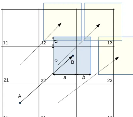
Sec-Figure 2.Scheme of Eulerian advection of sea ice. Points A and B denote start and end of drift of an ice parcel shown by the blue square.
ond, the SIA is computed, accounting for concentration of each ice age fraction.
3.1 Eulerian advection scheme
At each time step the observations of sea ice drift velocity components (UandV) and sea ice concentration (COBS) are provided as gridded products on the polar stereographic grid with the same spatial resolution with pixel size in x andy
directions equal toRx andRy, correspondingly. Uncertain-ties inU,V andCOBS products impact the accuracy of the end product but are not considered in the present study. We assume that a sample ice parcel in a pixel has shape of one grid cell and an initial ice concentrationC and correspond-ing velocity componentsUandV. An example is presented in Fig. 2, where the ice parcel originating from the pixel 31 is shown as a blue square. The parcel drifts from pointAover time1t and the coordinates of the destination pointB can be computed as follows:
XB=XA+U 1t
YB=YA+V 1t.
(1)
The areal fluxes of sea ice out of the donor pixel 31 into recipient pixels 12, 13, 22 and 23 are calculated as follows:
F31I12=C31ad, F31I13=C31bd, F31I22=C31ac, F31I23=C31bc,
(2)
where a,b,c andd are sides of the rectangles formed by intersection of the displaced donor pixel and recipient pixels
(Fig. 2). The recipient pixels are selected based on position of pointB – the four closest pixels become recipients. Con-centration of sea ice at the next step in a recipient pixel (e.g., pixel 13 in Fig. 2) (C13∗) is calculated as
C13∗ =F21I13+F22I13+F31I13+F32I13 (3) or in generalized form:
CR∗= X 4 donors
CD
1−|XR−XD−U 1t|
Rx
(4)
1−|YR−YD−V 1t|
Ry
,
whereCDis the concentration of a donor pixel,XD andYD are the coordinates of a donor pixel,XRandYRare the coor-dinates of the recipient pixels andRxandRyare pixel size.
When the observed sea ice drift field diverges then a gap appears between the ice parcels (e.g., in pixel 23). If the sum of fluxes (Eq. 4) into a recipient pixel falls behind the actu-ally observed concentration then this is interpreted as open-ing of leads, freezopen-ing of water in the leads and generation of new ice. Then, ice is presented by two fractions: the partial concentration of the older iceCOIis computed as the sum of incoming fluxes (Eq. 4) and the partial concentration of the young iceCYIis computed as a remainder:
CYI=COBS−COI. (5)
When the observed sea ice drift field converges then the advected ice parcels overlap (e.g., in the pixel 12) and the sum of fluxes into a recipient pixel may exceed the concen-tration observed by satellites. This is interpreted as genera-tion of pressure ridges and increase in thickness of the older fraction of sea ice. In that case the total ice concentration at the next step is assigned to be the observed ice concentration. During the freeze-up period the observed concentration in-creases and becomes higher than the sum of fluxes into a re-cipient pixel. This is also interpreted as generation of young ice (YI) only and Eq. (5) is used for computing YI concen-tration. During melting the observed concentration decreases and it may become less than the total predicted concentra-tion (sum of OI and YI fracconcentra-tions). In that case the YI con-centration is decreased first, and if YI is absent then the OI concentration is decreased.
3.2 Advection of sea ice age fractions
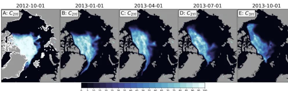
Figure 3.Example of advection of an ice fraction from 1 October 2012 to 1 October 2013 shown for every third month.
In our study we initiated SIA calculation on 1 Octo-ber 2012 when continuous high-quality observations of ice drift started to be available from AMSR2 (Fig. 3). For this date the total observed concentration was computed as the minimum concentration during the period 1 September– 1 October 2002. Propagation of ice age fractions from later years started from 10 September or respective years.
We did not know the spatial distribution of ice of differ-ent age within the pack at the first momdiffer-ent of time (1 Oc-tober 2012), but we can postulate that all observed ice is at least in the second-year ice (2YI) category. We have to make a simplification: the concentration of 2YI on 1 October 2012 is assigned to be equal to the total observed concentration:
C2YI=CTOT (Fig. 3a). Understandingly, this simplification allows us to initialize the SIA algorithm but does not allow to provide full SIA frequency distribution before a sufficiently long spin-up period (e.g., 5 years). Such a spin-up period is also needed for the NSIDC product. Then the developed ad-vection scheme is applied on a daily basis utilizing the avail-able daily ice drift and concentration products (Fig. 3b–e). From 1 October 2012 to 10 September 2013 (Fig. 3a–d) the advected fraction contains 2YI but on 10 September 2013 the age of this fraction is increased by 1 year and later it becomes the fraction of the third-year ice (3YI) (Fig. 3e).
On 10 September 2013 the total ice concentration is the sum of all MYI fractions and therefore the initial concentra-tion of the 2YI is calculated as
C2YI=CTOT−C3YI, (6)
where CTOT is the ice concentration observed by satellites andC3YIis the ice fraction advected from 1 October 2012. Both 2YI and 3YI fractions are advected further using the developed scheme and afterN years of advection on each of 10 September the concentration of 2YI is calculated as
C2YI=CTOT− X
i
Ci, (7)
whereCi is the concentration of the ice fraction advected from previous years.
3.3 Computation of sea ice age
At any moment of time, sea ice in each cell is characterized by a vector of concentrations of ice fractions of various age with the sum equal to the total sea ice concentration (Fig. 4). In other words the new algorithm provides ice age probability distribution. A single number that characterizes a probability density function can be computed in several standard ways: minimum, maximum, mean, median, mode, etc. We propose that SIA can also be computed from the concentration of ice age fractions using several approaches depending on the pre-ferred definition of the ice age (Fig. 5):
– Maximum ageis the age of the oldest ice fraction that exceeds a given threshold (e.g., 5 % concentration). – Average ageis the mean of age of the ice fraction that
exceeds a given threshold.
– Modal ageis the age of the ice fraction that has the high-est concentration.
– Median ageis the age of the ice fraction that splits the age distribution into two equal parts. Linear interpola-tion between the ice age fracinterpola-tions or approximainterpola-tion of ice distribution by a predefined function may be needed to compute median age correctly. More generally, me-dian (the value of the 50th percentile) can be replaced by any percentile.
– Weighted average ageis the average of ages of individ-ual ice fractions weighted by their concentrations:
A=
P fAfCf P
fCf
, (8)
Figure 4.Maps of sea ice age fractions on 1 March 2015.(a)Observed total sea ice concentration;(b–d)fractions of advected multi-year ice;(e) FYI fraction. Color bar represents the sea ice age fraction concentration.
Figure 5.Maps of sea ice age on 1 March 2015 computed with different methods.(a)Maximum ice age;(b)average ice age;(c)modal ice age;(d)weighted average ice age;(e)median (percentile 50) ice age;(f)NSIDC SIA. Color bar represents the sea ice age in years.
4 Results
The developed advection scheme (see Sect. 3.1) was applied to the sea ice drift and concentration products available at OSI SAF from 1 October 2012 to 1 March 2017. We com-pared our products to the already available sea ice products including SIA maps from NSIDC: time series and maps of MYI from NSIDC, Bremen University, OSI SAF and Den-mark Technological University (DTU). The results of com-parison presented below can be used for indirect assessment of our SIA algorithm.
4.1 Comparison with sea ice age product from NSIDC In order to provide stepwise illustration of the SIA product improvements we have used four different combinations of forcings and algorithms to produce a SIA map for the 1 Jan-uary 2016. First, we have implemented the NSIDC advection scheme (Lagrangian) and the SIA algorithm (age of the old-est parcel) and applied it to the ice drift product from NSIDC. Second, we have applied the NSIDC algorithms to the ice drift from OSI SAF. Third, we have applied our Eulerian
ad-vection scheme and SIA algorithm to the ice drift from OSI SAF but without accurately accounting for SIC. In this ex-periment all pixels with SIC below 15 % were assigned to be open water and other pixels contain 100 % ice. Finally, we have used the new advection scheme, the OSI SAF ice drift, and fully accounted for SIC.
Figure 6.Comparison of SIA for the 1 January 2016 calculated with the following combinations of forcings and algorithms:(a)NSIDC drift and NSIDC algorithm;(b)OSI SAF drift and NSIDC algorithm;(c)OSI SAF drift and SICCI algorithm without SIC;(d)OSI SAF drift and SICCI algorithm with SIC.
The change of the advection scheme does not affect the overall spatial distribution of MYI significantly (Fig. 6b and c) but generates a much smoother picture without dis-continuities. Using the weighted average for SIA computa-tion dramatically decreases the observed age (Fig. 6c). Few small spots where SIA reaches 4.5–5 years are observed only near the Canadian Archipelago and in the central Arctic. A stripe of high SIA appears along sea ice edge in the Fram Strait. This ice was advected from the central Arctic but frac-tions of younger ice have melted and only fracfrac-tions of older ice remain, making the weighted average value high.
When the new algorithm takes SIC into account then SIA is decreasing even more and the ice older than 4 years is ob-served only near the Canadian Archipelago coast (Fig. 6d). Moreover, extent of MYI is also decreased and the sleeves of 2YI towards the Laptev and Chukchi seas almost disappear. 4.2 Intercomparison of multi-year ice concentration
products
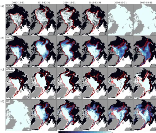
avail-Figure 7.Comparison of MYI concentration estimated from the NSIDC SIA product(a), from the SICCI SIA product(b), downloaded from OSI SAF(c)and from University of Bremen(d). Daily maps are generated for 31 December of the years from 2012 to 2016 and for 29 March 2017 from available data. Red contours denote extent of MYI in the SICCI product at 5 % concentration.
able from several resources including OSI SAF (Aaboe et al., 2017) and University of Bremen (Ye et al., 2016a). MYI can also be estimated from the NSIDC SIA product if we assume that bins with ice older than 1 year contain 100 % MYI and other bins contain 0 %. Total concentration of MYI from the SICCI product (with due consideration of SIC) was estimated as a sum of all multi-year fractions.
Intercomparison of MYI maps from four sources indicated that the general spatial distribution and temporal evolution is rather similar (Fig. 7): most of MYI is observed in the Canadian sector; a thin filament is exported through the Fram Strait; in some years the Beaufort Gyre advects MYI along
the Beaufort Sea coast; and sleeves of enhanced MYI con-centration are elongated towards the Laptev Sea.
discontinu-Figure 8.Seasonal dynamics of area of sea ice age fractions (filled plots) and multi-year ice area (dots) derived from the NSIDC product(a), from the SICCI product(b), from the UB product (black dots) and from the OSI SAF (yellow dots).
ous; generally it shows lower extent of MYI than other prod-ucts, but in some periods the extent is much higher (e.g., on 29 March 2017 in the Beaufort Sea). The UB product is also continuous and apparently can resolve smaller spatial details but the atmospheric influence seems to reduce MYI concen-tration in the middle of the ice pack (e.g., along the 150◦ meridian in 2013 or above the Yermak Plateau in 2015).
The time series of MYI areas are compared with regard to both seasonal dynamics (Fig. 8) and interannual variations (Fig. 9). Areas of ice age fractions of each age in the Arctic ocean are estimated individually from the NSIDC and SICCI products and plotted against time. For the NSIDC product the area of an ice age fraction is calculated as a number of all pixels corresponding to this ice age fraction multiplied by the area of the pixel. Similarly the MYI area from the OSI SAF product is estimated from the number of MYI pixels. For the SICCI product the area is estimated as the integral of the corresponding ice age fraction over all pixels. Similarly the MYI area from the UB product is estimated as the integral of MYI concentration over all pixels.
The seasonal variations of ice age fraction areas follow similar pattern for the NSIDC and SICCI products (Fig. 8): the sea ice area minimum (4×10⁶km2) is observed in mid-September, and it is followed by a rapid growth of the FYI (blue in Fig. 8) until the beginning of the next year. A sta-ble winter, when total area remain practically unchanged at level of 7–8×10⁶km2, is over in May and is followed by a rapid decrease of FYI. Unlike FYI, the area of MYI frac-tions cannot increase – it only gradually decreases due to
ice convergence and melting. Maximum area of the 2YI is also observed in mid-September – at this point all FYI from the previous year is considered as the ice which has survived summer melting and it becomes 2YI. Other fractions of older ice increase their age by 1 year in the same fashion.
The MYI area is shown in Figs. 8 and 9 as a demarca-tion of the blue and orange areas and as black and yellow dots. A comparison of MYI areas from the four products re-veals several differences. The NSIDC MYI area decreases in two regimes: a relatively slow decrease during winter solely due to convergence and a faster decrease at the end of spring when melting reaches MYI. The SICCI MYI area decrease also accelerates towards spring but more gently – melting affects MYI already starting from the beginning of spring. The MYI areas from UB and OSI SAF correspond well to the SICCI algorithm but exhibit much more sporadic vari-ability, including short periods of an inexplicable increase in MYI area. Although the MYI extent in the OSI SAF product is somewhat lower than of the other products (see maps in Fig. 7) the OSI SAF MYI area corresponds well to other es-timates (Figs. 8 and 9) because concentration of MYI within the ice extent is assumed to be 100 %.
Figure 9.Interannual dynamics of area of sea ice age fractions (bars) and multi-year ice area (dots) derived from NSIDC product (left bars), from NERSC product (right bars), from UB product (black dots) and from OSI SAF (black stars).
The interannual variability can be seen on the plot of areas of the ice age fractions for 1 January of 2013, 2014, 2015 and 2016 in Fig. 9. The total ice area (entire height of the columns) is lower for the SICCI product because it is calcu-lated as an integral ice concentration over all pixels whereas for the NSIDC it is calculated as sum of pixels within ice extent. The total MYI area is rather similar across the four products, but the area of older sea ice (≥2 years) fractions is lower by almost 20 % in the SICCI product.
4.3 Comparison of MYI with SAR
An independent validation of the SICCI MYI product was performed using a mosaic of synthetic aperture radar (SAR) images in HH polarization from Sentinel-1 A and B satellites acquired around 1 January 2016. MYI appears as brighter and more homogeneous texture on SAR images which al-lows one to draw an outline and compare it with outlines of MYI from the SICCI product as shown in Fig. 10. The SICCI MYI product corresponds very well to the SAR-derived MYI extent although it has much smoother boundaries due to low resolution of the input sea ice drift product (65 km). The low resolution is also the reason why SICCI MYI does not reach the coast, leaving a 50 km gap along the shoreline. The most considerable difference is observed in the Beau-fort Sea where the SAR-based MYI is seen as a stretched “archipelago” of MYI “islands”. In this area the SICCI prod-uct exhibits erroneously smooth decline in MYI concentra-tion and fills the gap between the MYI “archipelago” and the central Beaufort Sea.
Figure 10.Comparison of MYI extent derived by SAR visual inter-pretation (light blue) and from SICCI SIA product (red) on top of mosaic of Sentinel-1 SAR images for 1 January 2016. The thick red line shows 15 % threshold and thin red line shows 50 % threshold.
5 Discussion
Figure 11.Comparison of sea ice age for 1 January 1985 initiated from ice parcels with various density (1 parcel per 12×12 km, 6×6 km, 3×3 km).
the SIA and on the eventual application. For example, in our opinion, weighted average is the optimal method for graph-ical representation of SIA maps as it depicts the smooth na-ture of SIA distribution and accounts not only for the old-est ice fractions but also for the younger ones. However, for other applications, e.g., assimilation into models, a different method may be preferred. The SIA distribution can also be used to calculate MYI concentration for various applications, including calibration/validation of the PAMW-based MYI al-gorithms, improvement of the freeboard to sea ice thickness conversion for altimeter data and estimation of sea ice rough-ness for assimilation into models.
The motivation for implementing the Eulerian advection scheme in the new algorithm was to produce continuous and smooth spatial distributions of SIA fractions and also to pre-vent undersampling of the results. In the experiments with the NSIDC algorithm it was discovered that the density of starting points of the sea ice drift vectors indirectly influ-ences the area of MYI. Too low density (e.g., 1 drifter in each 12×12 km box as designed at NSIDC) leads to under-sampling of the ice age observations in the zone of strong di-vergence very early – only after a few years of propagation. With a two or four times higher number of initial points, un-dersampling is still experienced after 5 years of Lagrangian propagation. Observations that the Lagrangian approach in-troduces problems due to the dispersion of tracers were also previously reported in Rybak and Huybrechts (2003). The NSIDC method was run with three different initial densi-ties of ice parcels: one drifter per 12×12 km or 6×6 km or 3×3 km box. The results show that lower initial densities re-sult in a map of SIA with sparse presence of old ice fractions (Fig. 11a) and increasing the initial density of drift vectors leads to increase of concentration of the older ice (Fig. 11b and c). Consequently the area of older ice fractions≥6 years) increases and the area of younger ice fractions (≤5 years) decreases when the initial density is increased. Impact of the
increased initial density on increased MYI area is indepen-dent of the forcing and was demonstrated also for the OSI SAF ice drift field (not shown here).
The new sea ice drift product derived from AMSR2 also has a significant impact on the accuracy and reliability of the results. It accurately reproduces the sea ice circulation in the Arctic, is void of artifacts and produces homogeneous distri-bution of SIA fractions. It was discovered that the initial SID product is contaminated with high-frequency noise. Cleaning of SID with a median filter reduced small-scale deformations and prevented appearance of FYI discontinuities in artificial divergence zones. At the same time the low spatial resolu-tion of SID (65 km) limits the algorithm from reproducresolu-tion of fine-scale features in MYI distribution and may lead to over-smoothing in areas with high ice drift speed gradients (e.g., western Beaufort Sea).
con-straining by the SIC but more accurate estimates of long-term changes in the residence time will be possible when longer time series of the new SIA product become available.
The sea ice type algorithms based on PAMW satellite ob-servations have higher spatial resolution than the ice-drift-based algorithms but inevitably suffer from the unaccounted atmospheric impact or melt ponds and have to be corrected using information on air temperature or ice motion (Ye et al., 2016a, b). The method in our paper has high potential for complementing the PAMW algorithms and production of high-resolution and consistent MYI estimations. Such com-bined procedure can be realized, for example, as a machine learning algorithm which is trained to output SICCI MYI us-ing PAMW brightness temperatures (TB) as input. The ma-chine learning block can be realized as a simple polynomial regression or as a more complex neural network (Haykin, 1998). The training can be performed either on a per image basis, when only one mosaic of brightness temperatures is used as input and only one snapshot of MYI is used as out-put, or on a seasonal (or even satellite mission) basis, when information from many images is used for training. Alterna-tively, both SICCI MYI estimations and brightness tempera-tures can serve as input to classification algorithms, such as Bayesian classifier (Zhang, 2004) or support vector machines (Smola and Schölkopf, 2004).
6 Conclusions
We have developed a new algorithm for estimating sea ice age distribution using sea ice drift and concentration products. The algorithm is based on the Eulerian advection scheme which provides smooth distribution of the ice age pa-rameters and prevents the undersampling problem that may occur when a Lagrangian tracking approach is used. Another advantage of the selected scheme is the ability to generate not just a single age characteristic but a distribution of sea ice age fractions. First, this allows for flexibility in choosing the ice age definition and application of a statistical measure to compute SIA and, second, this provides individual spa-tial distributions of ice age fractions that can be assimilated into models or used for ice type delineation. For example, concentration of multi-year ice can be computed as a sum of multi-year ice fractions and used for defining ice density and snow thickness for the ice thickness algorithms, ice rough-ness for the ice circulation models and so on.
The new algorithm is driven by the new sea ice drift prod-ucts from OSI SAF, which is void of potential artifacts due to inclusion of autonomous ice drifter buoys. This leads to a more homogeneous distribution of ice age fractions over the Arctic Ocean. The algorithm is also constrained by the ob-served sea ice concentration from OSI SAF, which reduces fractions of old ice and, consequently, ice age by 20–30 %. It was applied to generate time series of daily sea ice age fraction product from October 2012 to October 2017.
Com-parisons with the NSIDC SIA time series indicate that the fractions of MYI in the new product melt faster during the year and after a spin-up time of 3 years the area of older ice in the SICCI product is almost 20 % lower than in the NSIDC product.
Data availability. The data generated with the algorithm are openly available at FTP (for bulk download; ftp://ftp.nersc.no/ ArcticData/esa_cci_sea_ice_age/) and at THREDDS (subsetting and online visualization; http://thredds.nersc.no/thredds/arcticData/ esa-cci-sea-ice-age.html) in netCDF format following CF conven-tions containing values of sea ice age fracconven-tions concentraconven-tions, MYI concentration, and sea ice age computed using weighted average (Korosov amd Rampal, 2018). Detailed information on datasets used in this paper can be found in Sect. 2.
Author contributions. AK developed and applied the presented al-gorithm, with contributions from PR. TL provided the new sea ice drift product. SA provided the OSI SAF ice type data. YY and GH provided the new sea ice type product. LTP and RS provided the mosaic of SAR images and multi-year ice outline. All co-authors participated in fruitful discussions and writing the manuscript.
Competing interests. The authors declare that they have no conflict of interest.
Acknowledgements. This work has been supported by the Sea Ice Age option of the Sea Ice Climate Change Initiative project funded by the European Space Agency, contract number 4000112229/15/I-NB.
Edited by: Jennifer Hutchings
Reviewed by: three anonymous referees
References
Aaboe, S., Breivik, L.-A., Sørensen, A., Eastwood, S., and Lavergne, T.: Global Sea Ice Edge and Type Product User’s Manual – v2.2, Tech. Rep. SAF/OSI/CDOP2/MET-Norway/TEC/MA/205, EUMETSAT OSI SAF – Ocean and Sea Ice Satellite Application Facility, available at: http://osisaf.met. no/docs/osisaf_cdop3_ss2_pum_sea-ice-edge-type_v2p2.pdf (last access: 13 June 2018), 2017.
Brodzik, M. J., Billingsley, B., Haran, T., Raup, B., and Savoie, M. H.: EASE-Grid 2.0: Incremental but Significant Improve-ments for Earth-Gridded Data Sets, ISPRS Int. Geo.-Inf., 1, 32– 45, https://doi.org/10.3390/ijgi1010032, 2012.
Fowler, C., Emery, W. J., and Maslanik, J.: Satellite-derived evolution of Arctic sea ice age: October 1978 to March 2003, IEEE Geosci. Remote S., 1, 71–74, https://doi.org/10.1109/LGRS.2004.824741, 2004.
Kwok, R. and Cunningham, G. F.: Variability of Arctic sea ice thickness and volume from CryoSat-2, Philos. T. R. Soc. A, 373, 20140157, https://doi.org/10.1098/rsta.2014.0157, 2015. Lavergne, T.: Algorithm Theoretical Basis Document for the
OSI SAF Low Resolution Sea Ice Drift Product – v1.3, Tech. Rep. SAF/OSI/CDOP/met.no/SCI/MA/130, EUMETSAT OSI SAF – Ocean and Sea Ice Sattelite Application Facility, available at: http://osisaf.met.no/docs/osisaf_cdop2_ss2_atbd_ sea-ice-drift-lr_v1p3.pdf (last access: 13 June 2018), 2016a. Lavergne, T.: Validation and Monitoring of the OSI SAF
Low Resolution Sea Ice Drift Product – v5, Tech. Rep. SAF/OSI/CDOP/met.no/T&V/RP/131, EUMETSAT OSI SAF – Ocean and Sea Ice Sattelite Application Facility, avail-able at: http://osisaf.met.no/docs/osisaf_cdop2_ss2_valrep_ sea-ice-drift-lr_v5p0.pdf (last access: 13 June 2018), 2016b. Lavergne, T., Eastwood, S., Teffah, Z., Schyberg, H., and Breivik,
L.-A.: Sea ice motion from low resolution satellite sensors: an alternative method and its validation in the Arctic, J. Geophys. Res., 115, C10032, https://doi.org/10.1029/2009JC005958, 2010.
Maslanik, J. A., Fowler, C., Stroeve, J., Drobot, S., Zwally, J., Yi, D., and Emery, W.: A younger, thinner Arctic ice cover: In-creased potential for rapid, extensive sea-ice loss, Geophys. Res. Lett., 34, L24501, https://doi.org/10.1029/2007GL032043, 2007. Maslanik, J. A., Stroeve, J., Fowler, C., and Emery, W.: Distribution and trends in Arctic sea ice age through spring 2011, Geophys. Res. Lett., 38, L13502, https://doi.org/10.1029/2011GL047735, 2011.
Perovich, D. K., Meier, W. N., Tschudi, M. A., Farrell, S. L., Ger-land, S., and Hendricks, S.: Sea Ice, in: Arctic Report Card 2015, Tech. rep., 2015.
Polyakov, I. V., Walsh, J. E., and Kwok, R.: Recent Changes of Arc-tic Multiyear Sea Ice Coverage and the Likely Causes, B. Am. Meteorol. Soc., 93, 145–151, https://doi.org/10.1175/BAMS-D-11-00070.1, 2012.
Rampal, P., Weiss, J., and Marsan, D.: Positive trend in the mean speed and deformation rate of Arctic sea ice, 1979–2007, J. Geophys. Res., 114, C05013, https://doi.org/10.1029/2008JC005066, 2009.
Rigor, I. G. and Wallace, J. M.: Variations in the age of Arctic sea-ice and summer sea-sea-ice extent, Geophys. Res. Lett., 31, L09401, https://doi.org/10.1029/2004GL019492, 2004.
Rybak, O. and Huybrechts, P.: A comparison of Eule-rian and Lagrangian methods for dating in
numer-Tonboe, R., Lavelle, J., Pfeiffer, H., and Howe, E.: Prod-uct User Manual for OSI SAF Global Sea Ice Con-centration Product OSI-401-b Version 1.6, Tech. Rep. SAF/OSI/CDOP3/DMI/MET/TEC/MA/204, EUMETSAT OSI SAF – Ocean and Sea Ice Satellite Application Facility, available at: http://osisaf.met.no/docs/osisaf_cdop3_ss2_pum_ ice-conc_v1p6.pdf (last access: 13 June 2018), 2017a.
Tonboe, R., Pfeiffer, H., Jensen, M., and Howe, E.: Vali-dation Report for OSI SAF Global Sea Ice Concen-tration Product OSI-401-b Version 1.6, Tech. Rep. SAF/OSI/CDOP2/DMI/SCI/RP/225, EUMETSAT OSI SAF – Ocean and Sea Ice Satellite Application Facility, available at: http://osisaf.met.no/docs/osisaf_cdop2_ss2_valrep_ice-conc_ v1p1.pdf (last access: 13 June 2018), 2017b.
Tschudi, M., Fowler, C., Maslanik, J., and Stroeve, J.: Track-ing the Movement and ChangTrack-ing Surface Characteristics of Arctic Sea Ice, IEEE J. Sel. Top. Appl., 3, 536–540, https://doi.org/10.1109/JSTARS.2010.2048305, 2010.
Tschudi, M., Fowler, C., Maslanik, J., Stewart, J. S., and Meier, W.: EASE-Grid Sea Ice Age, data set, NSIDC-0611, https://doi.org/10.5067/PFSVFZA9Y85G (last access: 1 September 2017), 2016a.
Tschudi, M., Fowler, C., Maslanik, J., Stewart, J. S., and Meier, W.: Polar Pathfinder Daily 25 km EASE-Grid Sea Ice Motion Vectors, Version 3, data set, NSIDC-0116, https://doi.org/10.5067/O57VAIT2AYYY (last access: 1 September 2017), 2016b.
Tschudi, M. A., Stroeve, J. C., and Stewart, J. S.: Relating the Age of Arctic Sea Ice to its Thickness, as Measured during NASA’s ICESat and IceBridge Campaigns, Remote Sens., 8, 457, https://doi.org/10.3390/rs8060457, 2016c.
World Meteorological Organization (WMO): Statement on the sta-tus of the global climate in 2015, WMO report No. 1167, 28 pp., available at: http://library.wmo.int/pmb_ged/wmo_1167_en.pdf (last access: 13 June 2018), 2016.
Ye, Y., Heygster, G., and Shokr, M.: Improving Multi-year Ice Concentration Estimates With Reanalysis Air Temperatures, IEEE T. Geosci. Remote, 54, 2602–2614, https://doi.org/10.1109/TGRS.2015.2503884, 2016a.
Ye, Y., Shokr, M., Heygster, G., and Spreen, G.: Improving Multi-year Sea Ice Concentration Estimates with Sea Ice Drift, Remote Sens., 8, 397, https://doi.org/10.3390/rs8050397, 2016b. Zhang, H.: The optimality of naive Bayes, American Association