https://doi.org/10.5194/amt-10-4805-2017 © Author(s) 2017. This work is distributed under the Creative Commons Attribution 4.0 License.
Continuous light absorption photometer for long-term studies
John A. Ogren1,2, Jim Wendell1, Elisabeth Andrews2, and Patrick J. Sheridan1
1Global Monitoring Division, Earth System Research Laboratory, National Oceanic and
Atmospheric Administration, Boulder, 80305, USA
2Cooperative Institute for Research in Environmental Sciences, University of Colorado,
Boulder, 80303, USA
Correspondence:John A. Ogren ([email protected]) Received: 23 June 2017 – Discussion started: 27 July 2017
Revised: 23 October 2017 – Accepted: 3 November 2017 – Published: 11 December 2017
Abstract.A new photometer is described for continuous de-termination of the aerosol light absorption coefficient, opti-mized for long-term studies of the climate-forcing proper-ties of aerosols. Measurements of the light attenuation co-efficient are made at blue, green, and red wavelengths, with a detection limit of 0.02 Mm−1 and a precision of 4 % for hourly averages. The uncertainty of the light absorption coef-ficient is primarily determined by the uncertainty of the cor-rection scheme commonly used to convert the measured light attenuation to light absorption coefficient and ranges from about 20 % at sites with high loadings of strongly absorb-ing aerosols up to 100 % or more at sites with low loadabsorb-ings of weakly absorbing aerosols. Much lower uncertainties (ca. 40 %) for the latter case can be achieved with an advanced correction scheme.
1 Introduction
Reliable observations of aerosol light absorption are crucial for quantifying the radiative forcing of climate. As a con-sequence, light absorption measurements are recommended for all stations in the Global Atmosphere Watch network, which is coordinated by the World Meteorological Organi-zation (World Meteorological OrganiOrgani-zation, 2016). Aerosol light absorption is often dominated by soot-like particles pro-duced by the incomplete combustion of carbonaceous fu-els, commonly termed “black carbon”. There are two basic approaches for determining the aerosol light absorption co-efficient, suspended-state methods, where the absorption is measured while the particles are suspended in air, and filter-basedmethods, where the particles are deposited on a filter
for real-time optical analysis. Suspended-state methods are inherently more accurate, because the physical state of the particles can be changed by the act of filtration, although both are subject to sampling artifacts associated with bringing particles from ambient conditions into a laboratory. Unfor-tunately, currently available instruments for suspended-state measurements are more expensive, less sensitive, and more difficult to operate than filter-based methods, making them better suited for use in intensive field campaigns or as lab-oratory reference instruments. Filter-based instruments, be-cause of their lower cost and simpler operation, have been the preferred choice for long-term observations of aerosol light absorption in monitoring networks.
NOAA has used filter-based instruments for measuring the aerosol light absorption coefficient at baseline observa-tories for over two decades. Both Aethalometers (Hansen et al., 1984) and Particle Soot Absorption Photometers (PSAP; Bond et al., 1999) have been used. These instruments, as well as the Multi-Angle Absorption Photometer (MAAP; Petzold and Schönlinner, 2004), lack one or more desirable features for long-term observations of the aerosol light absorption co-efficient for studies of aerosol forcing of climate. For exam-ple, the MAAP only measures at a single wavelength, the PSAP can require frequent (hourly to daily) filter changes, and the Aethalometer does not yet have a widely accepted correction scheme (see, e.g., Collaud Coen et al., 2010).
To address these issues, NOAA developed and built a filter-based instrument, the Continuous Light Absorption Photometer (CLAP), with the following design features:
smaller than 10 µm aerodynamic diameter; – precisely defined filter spot areas;
– optical configuration and filter media comparable to the PSAP, to allow use of the Bond et al. (1999) correction scheme for interfering effects caused by filter loading and multiple scattering;
– low cost and small size.
Unlike the MAAP, the CLAP does require a co-located aerosol light scattering or extinction measurement to derive aerosol light absorption.
This paper describes the CLAP model 10, so numbered be-cause it was originally designed in 2010. As the original de-sign evolved during development, several small adjustments were made to the prototype to provide the above features:
– A two-part design, where the top half must be manually removed to change the filter, was chosen to keep the mechanical design simple by eliminating the need for moving parts.
– O-rings for sealing the filter were eliminated, because the o-ring caused the edge of the spot to be diffuse and variable.
– A redesigned voltage regulator eliminated failures en-countered in the field.
– Use of a torque driver secured the top and bottom as-semblies after a filter change. The initial design used thumbscrews, but their uncontrolled torque sometimes resulted in incomplete sealing of the two assemblies. The CLAP contains an embedded microprocessor to mea-sure signals and control valves and heaters, but for simplicity the task of calculating the light absorption coefficient is del-egated to an external computer. A simple user interface and menu system are provided for manual or computerized con-trol of all CLAP functions.
ATN= −ln
I s
Ir
, (1)
and the time rate of change of attenuation yields the attenua-tion coefficient (σatn, m−1),
σatn=
A Q
(ATN(t2)−ATN(t1))
(t2−t1)
= A
Q 1ATN
1t , (2)
where ATN(t )is the filter attenuation at timest1andt2(in s),
Q(m3s−1)is the sample flow rate through the filter, andA (m2)is the area of the exposed spot on the filter.
The aerosol light absorption coefficientσapis derived from
the attenuation coefficient after corrections for changes in at-tenuation caused by light scattering from particles collected on the filter, multiple scattering and absorption of light within the filter medium, and reduction of the multiple-scattering ef-fect as the filter attenuation increases. These corrections for the PSAP were derived by Bond et al. (1999) and further elaborated by Ogren (2010):
σap=0.85
f (τ ) σatn
K2
−K1σsp
K2
, (3)
whereσspis the aerosol light-scattering coefficient adjusted
to the wavelength of the absorption measurement. The trans-mittance correction term is defined as
f (τ )=(1.0796τ+0.71)−1, (4) whereτ=(Is(t ) /Ir(t ) )(Is(0) /Ir(0) )is the normalized
filter transmittance at timet relative to transmittance at the start of sampling (t=0). The constants in Eq. (3) were derived by Bond et al. (1999) as K1=0.02±0.02 and
K2=1.22±0.20, where the uncertainties are given for the
95 % confidence level. The transmittance correction term, f (τ ), and K2 correct for the effects of filter loading and
multiple-scattering enhancement of absorption by particles within the filter matrix, while theK1-term corrects for the
An alternate correction scheme for the PSAP was reported by Virkkula et al. (2005) and Virkkula (2010).
The CLAP differs from the PSAP in that it utilizes solenoid valves to cycle through eight sample filter spots and two reference (i.e., unsampled) filter spots, enabling the in-strument to run at ideal conditions (filter transmittance, τ, greater than 0.7) eight times as long as the single-spot PSAP. The CLAP was designed to use 47 mm diameter, glass-fiber filters (Pallflex type E70-2075W), identical to the original PSAP filters except for size. These filters are made of two fibrous layers – borosilicate glass fibers overlaying a cellu-lose fiber backing material (for strength and stability). The cellulose fiber layer may take up water under conditions of high humidity, which is one reason that the CLAP has an internal heater to lower the sample relative humidity inside the instrument. The internal heater consists of two 78 ohm thin-film heaters glued to the bottom of the aluminum plate that holds the filter (Fig. 1). The temperature of this plate is measured with a thermistor and the microprocessor controls the power supplied to the heater in order to maintain the de-sired temperature. The plate temperature is normally set to 35–39◦C, which is sufficient to reduce the relative humidity to below 40 % most of the time. The temperature is typically maintained within 0.1◦C of the set point temperature, except in cases where the heat dissipated by the solenoid valves and electronics inside the CLAP is sufficient to cause the plate temperature to exceed the set point temperature; such cases occur in warm laboratories and require an operating temper-ature of 39◦C to achieve stable operation. Some losses of semi-volatile species might occur at these temperatures. The effects of such possible losses on the measured attenuation coefficient are unknown but assumed to be small because the dominant light-absorbing species (black carbon) is not volatile and the amount of heating is relatively small; how-ever, this is an area where further research would be useful.
A photograph and cutaway drawing of the CLAP opti-cal and flow paths, as well as the internal configuration, are shown in Fig. 1; an annotated version of Fig. 1b is included in the Supplement (Fig. S1). The round “top hat” contains the white hemisphere and LED light source, with the sample inlet tube located at the center. A manifold in the upper plate directs the sample flow to one of eight sample spots on the fil-ter below; miniature solenoid valves in the bottom part select the active sample spot. An external tube returns the filtered sample flow to the upper plate where it flows through one of the two reference spots, as selected by the miniature solenoid valves, to provide the measurement ofIr. The reference
mea-surement switches between the two reference spots each time the sample spot is changed because experience with the pro-totype instrument revealed that ATN drifts excessively dur-ing the first 10–20 min after a fresh sample spot is selected if the same reference spot is used. This drift is minimized if the reference spot is alternated, presumably because some time is needed for the reference spot to relax from the stretching caused by airflow through the filter. By switching the
refer-ence spot each time the sample spot is changed, both will stretch to roughly the same extent when exposed to the flow regime. If there were only one reference spot, that spot would already be stretched, leading to large ATN drift until the sam-ple spot reached a similar stretched state.
Diffuse sample illumination is provided by three sets of upward-facing light-emitting diodes (LED) in the upper half of the instrument. The LEDs illuminate the concave side of a white hemisphere, and the upward-facing detectors, in the lower half of the instrument, view this hemisphere through the sample deposit on the fiber filter. Because a parallel mea-surement of aerosol light-scattering coefficient is required for the calculation of the light absorption coefficient (Eq. 3), the wavelengths of the LEDs should match the wavelengths of the co-located scattering measurements as closely as possi-ble. However, LEDs of sufficient output intensity were not available at the TSI nephelometer (model 3563) wavelengths of 450, 550, and 700 nm, leading to the selection of LEDs with wavelengths of 468, 529, and 653 nm (see below).
A Texas Instruments MSP430F2618 microprocessor pro-vides the minimum functionality for measuring signals (light intensity reaching the 10 detectors, flow rate, case temper-ature, and sample temperature) and controlling the hard-ware (light source, case heater, and solenoid valves). The LEDs are cycled through four states (blue, green, red, dark) each second. Analog voltages from the detectors are dig-itized with 20-bit analog/digital converters (Texas Instru-ments DDC112); oversampling of the A/D converter in-creases the effective resolution to 22 bits. During develop-ment of the prototype CLAP, it became clear that noise lev-els of 1 Hz light intensities were unacceptably high and that some smoothing was needed. Consequently, a digital low-pass filter was implemented in the microprocessor software; the default filter is a four-stage, single-pole design with an effective first-order time constant of 2.6 s.
The internal software detects when the push button on the front panel is depressed and controls whether a red indicator lamp is lit or not; this lamp is off during normal sampling and on during a filter change. A blinking lamp indicates an error condition that must be corrected before continuing. A digital panel meter displays the sample flow rate, which is controlled by a needle valve; active flow control is not needed, as the flow rate typically varies by less than 1 % during sampling. Sensor calibration and configuration parameters are stored in nonvolatile memory and are accessible through a menu-based user interface via the RS232C serial port. An exter-nal computer is required for data logging, instrument control (e.g., switching to the next filter spot), and calculation of the attenuation coefficient.
Af-Figure 1. (a)Photograph of CLAP and(b)cross-sectional view of flow and optical paths in upper section and three-dimensional view of CLAP internal configuration in lower section. Scale on ruler on left image is in millimeters. An annotated version of(b)is included in the Supplement (Fig. S1).
ter each filter change, the upper half is secured to the lower half by tightening the four nuts to a torque of 2.5 N-m.
At NOAA federated network sites the CLAP is typically installed so that it draws its sample air through a modified TSI nephelometer (TSI, Inc., model 3563) blower bypass block. A drawing of the modified blower block is included in the Supplement (Fig. S2). This setup allows for the CLAP zero reading to be measured each time a nephelometer back-ground check with filtered air is performed (typically hourly at NOAA network sites). The vacuum for the CLAP is pro-vided by an external pump, which is typically a carbon vane pump.
3 Characterization
3.1 Particle sampling efficiency
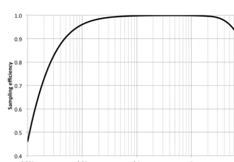
The internal flow paths through the CLAP were chosen to minimize losses of particles in the size range of 0.01–10 µm. Internal flow velocities at the design volumetric flow rate of 1.0 L min−1were 0.5–1 m s−1, with flow Reynolds num-bers of 230–300. A simplified model of the flow through the CLAP was used to estimate particle losses due to diffusion, impaction, and sedimentation. The combined particle sam-pling efficiency shown in Fig. 2 indicates that particle losses are less than 10 % for particles with aerodynamic diameters of 0.005–7 µm, and less than 1 % for 0.03–2.5 µm particles.
Figure 2.Calculated sampling efficiency of particles reaching the CLAP filter.
3.2 Wavelength response
Figure 3. Normalized spectral output of the light source for the blue, green, and red channels, and spectral sensitivity of the detec-tors (black curve).
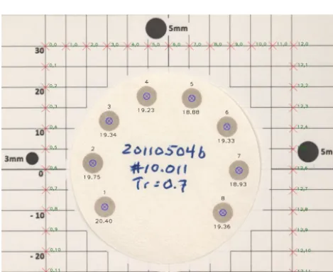
Figure 4.Example of photographic analysis of spot area. Numbers 1–8 above each spot indicate spot number, while the numbers below each spot indicate spot area in mm2.
3.3 Spot area
The spot areas were determined by an automated digital anal-ysis of photographs of exposed filters. The filters were placed on a grid with 5 mm line spacing, and photographs were taken with a high-resolution digital camera (12–16 megapix-els). The lens was an Olympus 60 mm f2.8 Macro (120 mm equivalent). The analysis program determined the pixel lo-cations of the grid intersection points and the approximate center of each spot, and then identified the outline of each spot based on the edge contrast. The area of each spot was calculated as the product of the number of pixels inside the outline and the size of each pixel. An example of the result-ing analysis is shown in Fig. 4.
Table 1.Spectral output characteristics of the light source. Values in parentheses are the coefficients of variation of measurements on 31 light sources. FWHM denotes the width of the curves at half the peak intensity.
Wavelength at Wavelength FWHM peak output (nm) centroid (nm) (nm) Blue 462.0 (0.3 %) 467.6 (0.5 %) 27.7 Green 522.3 (0.1 %) 528.7 (0.2 %) 39.8 Red 653.4 (0.1 %) 653.0 (0.1 %) 20.0
Each pixel in the 12 megapixel images was 23.8 µm square. A visual examination of the results of the automated image analysis revealed that the edge of the spots was iden-tified within one pixel; i.e., the uncertainty of the measured spot radius was 23.8 µm. This uncertainty corresponds to an uncertainty of the spot area of 1.9 %. Later images were taken with a 16 megapixel camera, yielding a spot area uncertainty of 1.6 %. For subsequent uncertainty calculations, we used a conservative estimate of the spot area uncertainty of 2 %.
The traditional method for measuring spot sizes relies on repeated measurements of the spot diameter by several ana-lysts using a magnifier and reticle. We measured the size of 12 spots manually (5 analysts, in a “blind” experiment where each analyst was unaware of the others’ results) and derived spot areas that were 1.3 % smaller than those derived with the automated image analysis, well within the combined uncer-tainty of the two methods. This limited study suggests that the uncertainty of the spot areas measured either manually or automatically is likely to be 2 % or lower.
The average area of 248 spots from a total of 31 individual instruments was 19.9 mm2with a coefficient of variation of 2.6 %. The averaged measured area is 14 % greater than the area of the 3/16 inch (4.76 mm) diameter holes that define the spots, suggesting that there may be a slight side leak-age flow in the fiber filters. Another possible reason for the slightly larger spot size is that the holes were deburred, yield-ing spot areas slightly larger than the machined hole. These possibilities reinforce the importance of measuring the spot areas rather than relying on internal dimensions.
3.4 Precision
Figure 5.Standard deviation of the attenuation coefficient measured by nine CLAPs (1 h averages, 529 nm wavelength). The line indi-cates the slope of the regression, forced through the origin.
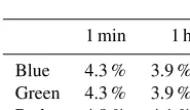
Table 2.Precision of the CLAP attenuation coefficients for 1 min and 1 h averaging times.
1 min 1 h Blue 4.3 % 3.9 % Green 4.3 % 3.9 % Red 4.8 % 4.1 %
The nine CLAP mass flow meters were calibrated prior to the experiment with a BIOS Definer 220M flow calibrator. The coefficient of variation of the repeated flow measure-ments with this calibrator in our laboratory was measured to be 0.2 %, which indicates that the flow calibration is not a major contributor to the overall CLAP precision. The calibra-tor manufacturer’s reported accuracy of 1 % is irrelevant for these precision tests, because the same flow calibrator was used for all instruments. However, the flow calibrator tainty should be included when calculating the overall uncer-tainty of the CLAP measurements.
3.5 Noise
The noise characteristics of each CLAP were measured as part of the manufacturing process as well as on occasions thereafter when the instruments were returned for servicing. In a typical noise test, the CLAP sample intensities and flow rates were recorded at 1 Hz for about 8 h on each spot while the instrument sampled filtered room air. The resulting time series for each spot was randomly sampled 500 times for se-lected averaging times 1t, (1 <1t< 104s) and the attenua-tion (Eq. 1) and attenuaattenua-tion coefficient (Eq. 2) were calcu-lated for each 1 s time step. The average attenuation coeffi-cient was calculated in two ways for each randomly chosen sample:
Figure 6.Standard deviation of the attenuation coefficient measured on filtered air as a function of averaging time. The thick black line with solid symbols represents the measurement data based on 8 h of measurements/spot; the thin black line with open symbols shows the measurement data when each spot was sampled for 1 week; the red line represents the approximate slope for 5–100 s averaging time; the blue line represents the approximate slope for 2 min to 1-day averaging times.
– arithmetic – the 1 Hz attenuation coefficients were aver-aged over the time interval1t;
– difference – the 1 Hz attenuation at the start and end times of the time interval1t was used to calculate the average attenuation coefficient from Eq. (2).
The standard deviation of the 500 random samples is inter-preted as the measurement noise associated with the averag-ing time1t.
Results from this analysis are shown as the thick black line in Fig. 6 for the arithmetic averages; the correspond-ing results for the difference-based averages were indistin-guishable from the arithmetic averages and are not shown. Furthermore, the results for the three wavelengths were very similar and so the figure shows the combined statistics for all wavelengths. The results represent a total of 3778 h of mea-surements using 28 different instruments. The statistics from this analysis are unreliable for averaging times longer than about 3 h, because the noise runs were generally around 8 h long. The error bars indicate the±1 standard deviation range of the results from all the different spots, instruments, and wavelengths for each averaging time; the lower bars for the rightmost points are not shown because the standard devia-tions were greater than the means for averaging times greater than 10 000 s (3 h).
sym-bols. The overlap between the two experiments for averag-ing times of 60–10 000 s indicates the consistency of the two approaches.
The slope of the curves in Fig. 6 is about −1 for aver-aging times of 10–100 s (red line) and about−0.5 for aver-aging times of 2–1440 min (blue line). For general use, the noise level of the CLAP attenuation coefficient can be ap-proximated as 0.10 Mm−1·(1t /100 s)n , with n= −1 for 5 s <1t <100 s andn= −0.5 for 100 s <1t <= 24 h. The overall statistics for 1 min averages yield a noise level of 0.19 Mm−1 with a coefficient of variation of 38 % for the 28 instruments tested (cf. 0.17 Mm−1 using the algorithm above).
Müller et al. (2011) reported noise levels of absorption co-efficients from six, 3-wavelength PSAPs of 0.06–0.07 Mm−1 for 1 min averages for all three wavelengths. The correspond-ing noise levels in terms of the attenuation coefficient are 0.13–0.15 Mm−1, i.e., slightly lower than the CLAP value
of 0.19 Mm−1. However, Müller et al. (2011) used an aver-aging method that was based on 1 min averages of the sam-ple intensities; i.e., the 1 min averages of the PSAP atten-uation coefficient used data from two consecutive minutes. As a consequence, it is appropriate to compare the noise from 2 min average attenuation coefficients for the CLAP (0.11 Mm−1)to the 1 min averages from the PSAP noise tests (ca. 0.14 Mm−1).
Springston and Sedlacek (2007, hereafter SS07) presented a comprehensive analysis of the PSAP noise characteristics. Many of their results are specific to the peculiarities of the internal data processing and serial output of the PSAP and are not applicable to the CLAP. In fact, one of the design goals for the CLAP was to implement straightforward inter-nal data processing and high-resolution serial data reports, as recommended by SS07, in order to avoid the limitations of the PSAP serial data reports. However, the results in Fig. 6 are comparable to the results for Case II reported in Fig. 4 of SS07, which show a noise level of 0.05 Mm−1 for 1 min averages of the single PSAP that was tested. The value of 0.05 Mm−1needs to be multiplied by the transmittance cor-rection factor f (τ )to convert it to the noise of the atten-uation coefficient. Assuming that SS07 measured the noise on blank filters (τ =1), their results correspond to a noise level of the attenuation coefficient of 0.09 Mm−1for 1 min averages, about half the magnitude of the CLAP noise. The source of the discrepancy between the PSAP noise levels re-ported by Müller et al. (2011) and SS07 is not understood, but might be a result of unit-to-unit variability (i.e., SS07 perhaps tested a PSAP with unusually low noise levels). As a result, about all that can be concluded is that the CLAP and PSAP noise levels are similar, to within a factor of 2.
The slope of the regression line relating log(noise) to log(averaging time) for the SS07 Case II is −1 for averag-ing times of 4–100 s, indistaverag-inguishable from the results for the CLAP shown in Fig. 6.
3.6 Measurement uncertainty
The uncertainty of the measured attenuation coefficient (Eq. 2) is given by
δσatn σatn = (5) v u u t δ1ATN 1ATN 2 noise + δσ atn σatn 2 precision + δQ Q 2 ,
whereδXdenotes the uncertainty ofX. Equation (5) assumes that the uncertainty of the measurement interval1t is negli-gible. The 2 % uncertainty of the spot area is implicitly in-cluded in the 4 % precision of the CLAP measurements and should not be counted twice. As a result, the uncertainty of the measured attenuation coefficient, including the 4 % pre-cision and the 1 % uncertainty of the flow calibration, is cal-culated as δσatn σatn = s δ1ATN 1ATN 2 noise
+(0.01)2+(0.04)2
= s δσ atn σatn 2 noise
+(0.041)2. (6)
The noise term in Eq. (6) is calculated from the noise mea-surements described in Sect. 3.6, as shown in Fig. 6. Applica-tion of Eq. (6) for different attenuaApplica-tion coefficients and aver-aging times yields the relative uncertainty in the attenuation coefficient, expressed at the 95 % confidence level, as a func-tion of averaging time and attenuafunc-tion coefficient (Fig. 7). For hourly averages and attenuation coefficients larger than 2 Mm−1, the uncertainty of the attenuation coefficients mea-sured by the CLAP is 8 %, determined entirely by the flow calibrator accuracy and the CLAP precision.
The uncertainty of the absorption coefficient (Eq. 3) can be written as
δσap σap = 1 K2 (7) v u u
t(K2+aK1)2 " δσatn σatn 2 noise
+(0.41)2 #
+(aδK1)2+(δK2)2,
where a=$0/ (1−$0) and $0=σsp/ σsp+σap is the
single-scattering albedo. The quantity in square brackets in Eq. (7) is the uncertainty of the attenuation coefficient (Eq. 6), and the uncertainties of the parameters of the Bond et al. (1999) correction areδK1=0.01 andδK2=0.1 (at the
Figure 7.Uncertainty of CLAP measurements of the attenuation coefficient as a function of averaging time and attenuation coeffi-cient, expressed as the 95 % confidence level.
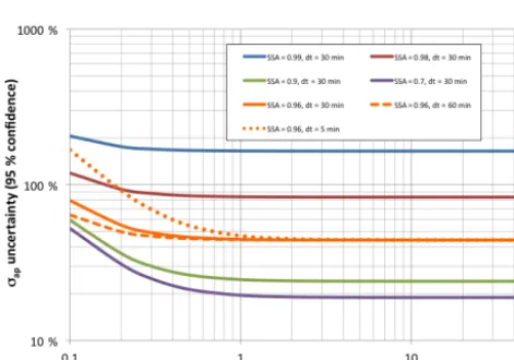
Figure 8.Uncertainty of CLAP measurements of the absorption efficient (95 % confidence level) as a function of the attenuation co-efficient, for various values of the single-scattering albedo (SSA) and averaging time (dt). Solid lines are all for 30 min averaging time, dashed lines are for other averaging times as noted in the leg-end.
et al. (1999) correction for averaging times of 5 min or more and attenuation coefficients of 1 Mm−1or more. The results in Fig. 8 are consistent with the results derived for the PSAP by Müller et al. (2014, Fig. 14b).
Equation (7) shows that values of both the single-scattering albedo and attenuation coefficient are needed to derive the uncertainty of the absorption coefficient, which precludes giving a single value for the uncertainty of the ab-sorption coefficient for ambient aerosol measurements. How-ever, NOAA and collaborators have operated CLAPs at a va-riety of sites with a wide range of single-scattering albedos and attenuation coefficients, which allows calculation of the frequency distribution of the uncertainty of the absorption coefficients measured at those sites. Figure 9 illustrates the
Figure 9.Percent uncertainty of the 30 min average light absorp-tion coefficient as a funcabsorp-tion of single-scattering albedo and atten-uation coefficient. The median uncertainty and interquartile range are shown for values measured for 2013–2016 at eight sites (ARN, El Arenosillo, Spain; BND, Bondville, USA; BRW, Barrow, USA; GSN, Gosan, South Korea; LLN, Mt. Lulin, Taiwan; MLO, Mauna Loa, Hawaii; SUM, Summit, Greenland; THD, Trinidad Head, USA). Uncertainties are given at the 95 % confidence level.
uncertainty of the derived absorption coefficient at 95 % con-fidence calculated using Eq. (7) for 30 min averages, along with the interquartile range of the single-scattering albedo and attenuation coefficient for eight sites. An averaging time of 30 min was chosen because these sites (except SUM) em-ploy switched impactors to measure both PM10and PM1size
ranges over the course of 1 h, and so the hourly averages from these stations are based on about 30 min of data for each size cut. The station-specific results in Fig. 9 are combined values for all three wavelengths of the CLAP and for both the PM10
and PM1size ranges, for the 4-year period 2013–2016. The
lowest uncertainties are seen for stations with greater absorp-tion and lower single-scattering albedo (e.g., ARN, GSN) and the highest uncertainties are seen when absorption is low and single-scattering albedo is high (e.g., BRW). The overall median uncertainty of the derived absorption coefficient for these eight stations is 30 %, and 75 % of the time the uncer-tainty is below 49 %.
The uncertainties shown in Fig. 9 are primarily deter-mined by the uncertainty of theK1 and K2 parameters of
the Bond et al. (1999) correction scheme. An advanced cor-rection scheme, the constrained two-stream (CTS) method reported by Müller et al. (2014), yields much lower uncer-tainties for weakly absorbing aerosols, with unceruncer-tainties re-duced to about 30 % for a single-scattering albedo of 0.98. 3.7 Comparison with PSAP
LLN (red) N = 39320
Slope = 0.72 ± 0.000 Intercept = −0.002 ± 0.001 0
10 20 30 40
0 20 40 60
PSAP attenuation coefficient (Mm−1)
CLAP atten
uation coefficient (Mm
−
1)
(a)
APP (red) N = 32263
Slope = 0.85 ± 0.001 Intercept = −0.022 ± 0.003 0
4 8 12
0 5 10
PSAP attenuation coefficient (Mm−1)
CLAP atten
uation coefficient (Mm
−
1)
(b)
THD (red) N = 11788
Slope = 0.97 ± 0.003 Intercept = 0.100 ± 0.003 −2
0 2 4
−2 0 2 4
PSAP attenuation coefficient (Mm−1)
CLAP atten
uation coefficient (Mm
−
1)
(c)
THD (blue) N = 11738
Slope = 1.06 ± 0.002 Intercept = 0.164 ± 0.003 −3
0 3 6
−2.5 0.0 2.5 5.0 7.5
PSAP attenuation coefficient (Mm−1)
CLAP atten
uation coefficient (Mm
−
1)
(d)
Figure 10.Comparison of attenuation coefficients measured with CLAP and PSAP at three stations(a)LLN, Mt. Lulin, Taiwan;(b)APP, Appalachian State University, Boone, NC, USA; (c)THD, Trinidad Head, CA, USA;(d)THD, blue wavelength. Results are for the red wavelength, except for(d). The shaded areas contain 90 % of the observations and the color shading distinguishes the deciles of the two-dimensional probability distribution function of the measurements. The orthogonal regression lines are shown in blue and the 1:1 line is gray and dashed. Slopes and intercepts of the orthogonal regression lines are included along with their uncertainties (95 % confidence) and the number of hourly observations (N); the regression lines account for over 98 % of the variance in each data set.
of parallel operation with the existing PSAPs was required before the PSAPs were retired from service. The resulting data set for a statistical comparison of the CLAP and PSAP measurements is comprised of 27 station-years of data from 17 stations. An example of the comparison for four stations, spanning the full range of the regression slopes, is shown in Fig. 10. The PSAP and CLAP filter changes were not syn-chronized for these comparisons, resulting in different trans-mittances reported by the two instruments. The transmittance correction factorf (τ )(Eq. 4) was applied to the attenuation coefficients calculated with Eq. (2) to put the two measure-ments on a comparable basis. The regression analysis was done with a principal component technique that minimizes the orthogonal distance to the regression line so that uncer-tainties in both the x- andy-variables are considered. The final analysis excluded points that are more than three stan-dard deviations from the regression line to reduce the sensi-tivity to outliers. Intercepts of the regression lines were gen-erally small (median−0.02 Mm−1, mean 0.04 Mm−1)with respect to the noise level of hourly averages from the CLAP (0.035 Mm−1at 95 % confidence) and so were neglected for the following analysis. However, a least-squares linear
re-gression analysis, with the rere-gression line forced through the origin, was also performed: the resulting regression line slopes were, on average, within 1 % of the slopes of the or-thogonal regression. The results from the oror-thogonal regres-sion analysis are considered to be more representative of the quantitative relationship between the CLAP and PSAP atten-uation coefficients because the analysis allows for variations in both variables, whereas ordinary least-squares analysis al-lows for variations in only the independent variable.
The analysis exemplified in Fig. 10 was repeated for all stations and wavelengths. The average slopes of the regres-sion lines were 0.95, 0.92, and 0.86 for the blue, green, and red wavelength channels, respectively; the overall mean slope was 0.91 with a standard deviation of 0.10. The regres-sion slopes are plotted in Fig. 11 as a function of the mean attenuation coefficient.
Figure 11.Slope of orthogonal regression line relating attenuation coefficients measured by CLAP vs. PSAP as a function of mean attenuation coefficient for 17 stations. The blue line indicates the median slope of 0.914. Data are given for all measured wavelengths.
than the PSAP results for the blue, green, and red mea-surement wavelengths, respectively. No correction for these slight differences is made in the CLAP-PSAP comparison re-ported here.
A comprehensive evaluation of the precision and noise level of PSAP measurements is not available, although the limited evaluations that have been published (Bond et al., 1999; Müller et al., 2011) suggest that the uncertainty of the attenuation coefficients measured with the PSAP is probably similar to, and perhaps somewhat greater, than that derived here for the CLAP. Assuming that the two measurements each have a comparable uncertainty of 10 % and disregarding the contribution of measurement noise, then the resulting un-certainty of the ratio of the two measurements is 14 % (95 % confidence bound). The average ratio of 0.91 derived here is thus indistinguishable from unity with better than 95 % con-fidence, indicating that measurements of the attenuation co-efficient with the CLAP and PSAP are equal within the un-certainty of the measurements.
4 Operation with alternative filter
The Pallflex E70-2075W filters are no longer commercially available so a replacement filter (model 371M, Azumi Fil-ter Paper Co., Japan) has been investigated. These filFil-ters were evaluated by Irwin et al. (2015) for use in the COS-MOS. Irwin et al. (2015) developed an alternative transmit-tance correction f (τ ) for COSMOS and compared results from 10 days of parallel operation of two COSMOS units in Tokyo equipped with Azumi and Pallflex filters. They re-ported that black carbon concentrations measured by COS-MOS with Azumi filters were 6–8 % higher than the values measured with Pallflex filters, depending on the transmit-tance correction used. The 6–8 % difference in black carbon
ters. These experiments do not represent a comprehensive evaluation of the CLAP response to Azumi filters but rather a study of the feasibility of using Azumi filters in the CLAP; a more comprehensive evaluation will be the subject of a future paper. The first experiment sampled ambient air in Boulder, Colorado, while the second sampled nebulized and dried Regal Black particles (REGAL R400 pigment black, Cabot Corp., USA) in the laboratory. In both experiments, one CLAP used the Pallflex E70-2075W filter and the sec-ond CLAP used the Azumi 371M filter. The raw CLAP data were corrected in real-time using the measured spot areas and flow calibrations, and 1 min averages were recorded. The slope of the regression line of the attenuation coefficients measured on Azumi vs. Pallflex filters, forced through the origin, was calculated using three different transmittance cor-rections: no correction,f (τ )from the Bond et al. (1999) cor-rection (Eq. 4), and the alternative corcor-rections derived for COSMOS by Irwin et al. (2015). Separate equations were used for Pallflex and Azumi filters for the latter case (Eqs. 10 and 11, respectively, from Irwin et al., 2015). Linear regres-sions were performed on trimmed data, where only the cen-tral 95 % of the data were considered. The linear regression line was forced through the origin, because the unforced re-gression lines all had intercepts very close to zero. Results obtained from the two filters were highly correlated, with co-efficients of determination of 0.98 or greater.
The ambient measurements used in this comparison were made from 2 December 2015 to 19 February 2016. Approx-imately 100 000 1 min average values were available for the comparison. The laboratory measurements on Regal Black were of much shorter duration, consisting of about 300 min of data from three runs when the transmittance on the Pallflex filters decreased from 1 to about 0.5.
Light attenuation coefficients measured on the Azumi fil-ters were consistently about 25 % greater than those mea-sured on the Pallflex filters, regardless of the scheme used to correct for the dependence on instrument response on fil-ter loading (Table 3). This difference is likely due to dif-ferent physical and optical properties of the filters, e.g., pore size, fiber diameter, particle penetration depth, and multiple-scattering characteristics. The results from Boul-der are consistent with Irwin et al.’s results from Tokyo in showing that the different correction schemes do not cre-ate a large difference in the ratio of light absorption coeffi-cients (or equivalent black carbon mass concentration). How-ever, the Azumi/Pallflex light attenuation ratios measured with CLAPs in Boulder (ca. 1.25) are substantially greater than the ratios measured with COSMOS in Tokyo (ca. 1.05). Some possible hypotheses that explain the different results from Boulder compared to Tokyo are as follows:
– The light absorbing particles in Boulder are different from those in Tokyo.
– There are sampling issues, such as different particle losses downstream of each instrument inlet.
– The powerful heater in COSMOS alters the particles in a way that changes the filter response.
– The optics in the CLAP and COSMOS are different. Further experiments are needed to test these hypotheses.
5 Conclusions
The CLAP has proven to be a reliable instrument for deter-mining the aerosol light absorption coefficient under a wide variety of sampling conditions, including from research air-craft (Aliabadi et al., 2015; Backman et al., 2016; Sherman et al., 2015; Schmeisser et al., 2017; Sinha et al., 2017; Sor-ribas et al., 2017). The two-part design, with the associated need to separate the two halves for each filter change, has been mostly problem-free. Likewise, the need for a torque driver to bind the two parts together has not been an oper-ational hurdle. With its small internal heaters, sensitivity to sample temperature and relative humidity is much reduced compared to the PSAP. Filter changes are typically needed once per month at remote sites, once or twice per week at ru-ral continental sites, and daily at very polluted sites. Compar-ison of attenuation coefficients measured with the CLAP and PSAP at 17 sites indicates that the results are equal within the uncertainty of the measurements.
As of mid-2017, 22 CLAPs have been deployed at long-term monitoring sites operated by NOAA and its partners. A commercial version of the CLAP, called the Tri-color Absorption Photometer (TAP, Brechtel Manufacturing, Inc., Hayward, CA, USA), is now available, and production of
Table 3.Ratio of the light attenuation coefficient measured with Azumi filter to the value measured with Pallflex filter.
Transmittance correction Ambient Black No correction 1.25 1.21 Bond et al. (1999) 1.30 1.25 Irwin et al. (2015) 1.26 1.21
CLAPs at NOAA is expected to wind down as a result. Eval-uation of the TAP response to laboratory and urban aerosols will be the subject of a future paper.
The Pallflex filter originally used in the CLAP and PSAP is no longer available. Limited tests with a replacement filter (Azumi 371M) show a high correlation between the two filter types, with the Azumi filter yielding attenuation coefficients that are about 25 % higher than the Pallflex filter. Further research is needed to assess whether a different correction scheme will be needed for the Azumi filter.
Code availability. Technical information on the CLAP, includ-ing construction drawinclud-ings, schematics, printed circuit board layouts, and source code, are available upon request from [email protected], under the terms of the GNU General Public License v2.
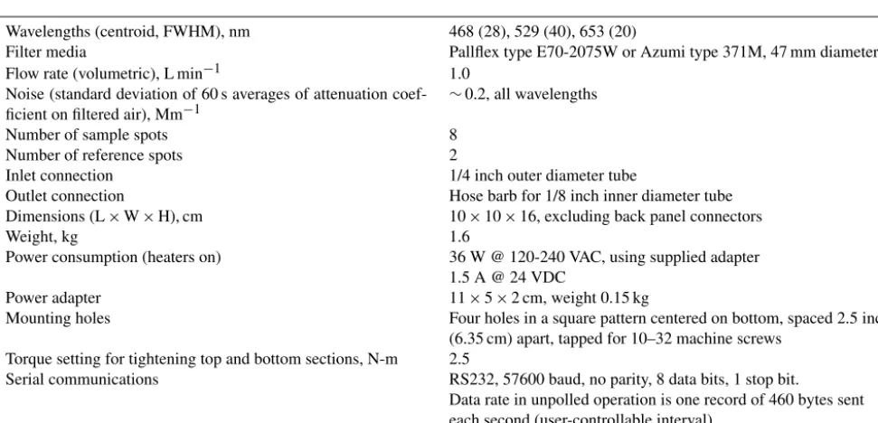
Dimensions (L×W×H), cm 10×10×16, excluding back panel connectors
Weight, kg 1.6
Power consumption (heaters on) 36 W @ 120-240 VAC, using supplied adapter 1.5 A @ 24 VDC
Power adapter 11×5×2 cm, weight 0.15 kg
Mounting holes Four holes in a square pattern centered on bottom, spaced 2.5 inch (6.35 cm) apart, tapped for 10–32 machine screws
Torque setting for tightening top and bottom sections, N-m 2.5
Serial communications RS232, 57600 baud, no parity, 8 data bits, 1 stop bit.
The Supplement related to this article is available online at https://doi.org/10.5194/amt-10-4805-2017-supplement.
Author contributions. JO designed the experiments and JO, PS and EA carried them out. JW designed and built the instruments, and wrote the operating software. JO prepared the manuscript with con-tributions from all co-authors.
Competing interests. The authors declare that they have no conflict of interest.
Disclaimer. The scientific results and conclusions, as well as any views or opinions expressed herein, are those of the author(s) and do not necessarily reflect the views of NOAA or the Department of Commerce. The mention of a commercial company or product does not constitute an endorsement by the NOAA Global Monitor-ing Division. Use of information from this publication concernMonitor-ing proprietary products or the test of such products for publicity or advertising purposes is not authorized.
Acknowledgements. The authors are grateful to Wilfred von Dauster for taking the photograph for spot size determination, Derek Hageman for writing the data acquisition software and assisting with data analysis, Anne Jefferson for comments on the draft manuscript, Katy Sun for assistance in preparing figures, James Sherman for providing data from APP, Mar Sorribas for providing data from ARN, Sang-Woo Kim for providing data from GSN, and Neng-Huei Lin and the Taiwan EPA for providing data from LLN. Funding of this effort was provided by the NOAA Climate Program Office.
Edited by: Willy Maenhaut
Reviewed by: three anonymous referees
References
Aliabadi, A. A., Staebler, R. M., and Sharma, S.: Air quality mon-itoring in communities of the Canadian Arctic during the high shipping season with a focus on local and marine pollution, At-mos. Chem. Phys., 15, 2651–2673, https://doi.org/10.5194/acp-15-2651-2015, 2015.
Backman, J., Schmeisser, L., Virkkula, A., Ogren, J. A., Asmi, E., Starkweather, S., Sharma, S., Eleftheriadis, K., Uttal, T., Jefferson, A., Bergin, M., and Makshtas, A.: On Aethalome-ter measurement uncertainties and multiple scatAethalome-tering en-hancement in the Arctic, Atmos. Meas. Tech. Discuss., https://doi.org/10.5194/amt-2016-294, in review, 2016. Bond, T. C., Anderson, T. L., and Campbell, D.: Calibration and
intercomparison of filter-based measurements of visible light ab-sorption by aerosols, Aerosol Sci. Tech., 30, 582–600, 1999. Collaud Coen, M., Weingartner, E., Apituley, A., Ceburnis, D.,
Fierz-Schmidhauser, R., Flentje, H., Henzing, J. S., Jennings, S.
G., Moerman, M., Petzold, A., Schmid, O., and Baltensperger, U.: Minimizing light absorption measurement artifacts of the Aethalometer: evaluation of five correction algorithms, Atmos. Meas. Tech., 3, 457–474, https://doi.org/10.5194/amt-3-457-2010, 2010.
Hansen, A. D. A., Rosen, H., and Novakov, T.: The aethalometer – An instrument for the real-time measurement of optical absorp-tion by aerosol particles, Sci. Total Environ, 36, 191–196, 1984. Irwin, M., Kondo, Y., and Moteki, N.: An empirical cor-rection factor for filter-based photo-absorption black carbon measurements, J. Aerosol Sci., 80, 86–97, https://doi.org/10.1016/j.jaerosci.2014.11.001, 2015.
Kondo, Y., Sahu, L., Kuwata, M., Miyazaki, Y., Takegawa, N., Moteki, N., Imaru, J., Han, S., Nakayama, T., Kim Oanh, N. T., Hu, M., Kim, Y. J., and Kita, K.: Stabilization of the mass ab-sorption cross section of black carbon for filter-based abab-sorption photometry by the use of a heated inlet, Aerosol Sci. Tech., 43, 741–756, https://doi.org/10.1080/02786820902889879, 2009. Müller, T., Henzing, J. S., de Leeuw, G., Wiedensohler, A.,
Alastuey, A., Angelov, H., Bizjak, M., Collaud Coen, M., En-gström, J. E., Gruening, C., Hillamo, R., Hoffer, A., Imre, K., Ivanow, P., Jennings, G., Sun, J. Y., Kalivitis, N., Karlsson, H., Komppula, M., Laj, P., Li, S.-M., Lunder, C., Marinoni, A., Mar-tins dos Santos, S., Moerman, M., Nowak, A., Ogren, J. A., Pet-zold, A., Pichon, J. M., Rodriquez, S., Sharma, S., Sheridan, P. J., Teinilä, K., Tuch, T., Viana, M., Virkkula, A., Weingart-ner, E., Wilhelm, R., and Wang, Y. Q.: Characterization and in-tercomparison of aerosol absorption photometers: result of two intercomparison workshops, Atmos. Meas. Tech., 4, 245–268, https://doi.org/10.5194/amt-4-245-2011, 2011.
Müller, T., Virkkula, A., and Ogren, J. A.: Constrained two-stream algorithm for calculating aerosol light absorption coefficient from the Particle Soot Absorption Photometer, Atmos. Meas. Tech., 7, 4049–4070, https://doi.org/10.5194/amt-7-4049-2014, 2014.
Ogren, J. A.: Comment on calibration and intercompar-ison of filter-based measurements of visible light ab-sorption by aerosols, Aerosol Sci. Tech., 44, 589–591, https://doi.org/10.1080/02786826.2010.482111, 2010.
Ogren, J. A.: Data files for CLAP paper figures and tables, available at: ftp://aftp.cmdl.noaa.gov/data/aer/papers/Ogren_2017_AMT_ CLAP, last access: 6 December 2017.
Petzold, A. and Schönlinner, M.: Multi-angle absorption photometry–a new method for the measurement of aerosol light absorption and atmospheric black carbon, J. Aerosol Sci., 35, 421–441, 2004.
Schmeisser, L., Andrews, E., Ogren, J. A., Sheridan, P., Jefferson, A., Sharma, S., Kim, J. E., Sherman, J. P., Sorribas, M., Kalapov, I., Arsov, T., Angelov, C., Mayol-Bracero, O. L., Labuschagne, C., Kim, S.-W., Hoffer, A., Lin, N.-H., Chia, H.-P., Bergin, M., Sun, J., Liu, P., and Wu, H.: Classifying aerosol type using in situ surface spectral aerosol optical properties, Atmos. Chem. Phys., 17, 12097–12120, https://doi.org/10.5194/acp-17-12097-2017, 2017.