www.geosci-model-dev.net/5/1395/2012/ doi:10.5194/gmd-5-1395-2012
© Author(s) 2012. CC Attribution 3.0 License.
Geoscientific
Model Development
Implementation of multirate time integration methods for air
pollution modelling
M. Schlegel1, O. Knoth1, M. Arnold2, and R. Wolke1
1Leibniz Institute for Tropospheric Research, Permoserstraße 15, 04318 Leipzig, Germany
2Martin Luther University Halle-Wittenberg, Institute of Mathematics, 06099 Halle (Saale), Germany Correspondence to: R. Wolke ([email protected])
Received: 11 July 2011 – Published in Geosci. Model Dev. Discuss.: 15 November 2011 Revised: 5 September 2012 – Accepted: 9 October 2012 – Published: 12 November 2012
Abstract. Explicit time integration methods are charac-terised by a small numerical effort per time step. In the appli-cation to multiscale problems in atmospheric modelling, this benefit is often more than compensated by stability problems and step size restrictions resulting from stiff chemical reac-tion terms and from a locally varying Courant-Friedrichs-Lewy (CFL) condition for the advection terms. Splitting methods may be applied to efficiently combine implicit and explicit methods (IMEX splitting). Complementarily multi-rate time integration schemes allow for a local adaptation of the time step size to the grid size. In combination, these ap-proaches lead to schemes which are efficient in terms of eval-uations of the right-hand side. Special challenges arise when these methods are to be implemented. For an efficient im-plementation, it is crucial to locate and exploit redundancies. Furthermore, the more complex programme flow may lead to computational overhead which, in the worst case, more than compensates the theoretical gain in efficiency. We present a general splitting approach which allows both for IMEX split-tings and for local time step adaptation. The main focus is on an efficient implementation of this approach for parallel com-putation on computer clusters.
1 Introduction
Atmospheric processes can be described using advection-diffusion-reaction equations. The advection term describes transport due to wind, diffusion describes turbulent mixing on spatial scales below the cell size. Both of these terms can efficiently be solved using explicit Runge-Kutta (RK) methods. So called Runge-Kutta-Chebychev methods were
developed for the coupled treatment of advection-diffusion problems (Verwer, 1996), (Verwer et al., 2004). Depend-ing on the specific simulation, the reaction terms may de-scribe microphysical processes or chemical reactions of pol-lutants including source terms. These terms are usually stiff as characteristic times of involved processes differ signifi-cantly. Employing explicit methods is not efficient in this case as stability requirements limit the time step size to un-practically small values. Implicit methods have proven to be much more efficient for the chemistry problem.
Implicit/explicit (IMEX) splittings have been developed which allow for an efficient solution of advection-diffusion-reaction equations. Complementarily since the 1980s ex-plicit multirate methods have been developed (e.g., Osher and Sanders, 1983; Tang and Warnecke, 2005) which allow for efficient solution of problems which can be split into non-stiff sub-systems with differing characteristic times, for ex-ample, advection on locally refined grids. Generally, multi-rate schemes result only in a significant reduction of com-putational costs if the amount to compute the part which re-quires smaller time steps is low in comparison to the total effort.
In the majority of current atmospheric models simple op-erator splittings are employed while the usage of multirate methods is rare. In Schlegel et al. (2009, 2012) we presented a generic splitting approach which can be employed to struct a multirate-IMEX scheme. The current paper is con-cerned with the efficient implementation of this scheme in the state-of-the-art Multiscale Atmospheric Chemistry and Transport model COSMO-MUSCAT (Wolke et al., 2004; Hinneburg et al., 2009) developed at the Institute for Tro-pospheric Research in Leipzig.
The remainder of this paper is structured as follows. First, we will mathematically outline a generic splitting scheme. The subsequent section is concerned with the focus of this paper, i.e., details of a practical implementation. We shall present the programme flow, details on data exchange and a balancing approach in separate subsections. Finally, we present two scenarios and discuss the obtained reduction of computational cost for each of them.
2 Mathematical preliminaries
In Schlegel et al. (2009) we presented a general splitting that may be employed to generate multirate methods, called re-cursive flux splitting multirate (RFSMR). The approach is based on an IMEX splitting presented by Knoth and Wolke (1998a), which we briefly outline here. These schemes can be seen as a higher-order generalisation of the popular source splitting approach (Verwer et al., 2002). Consider an equa-tion
w0=F (w)+G(w).
In the context of this paperGrepresents advection with com-paratively low Courant numbers. The other term,F, may rep-resent diffusion-reaction or advection with higher Courant numbers.
Denote the time substeps in the explicit method byτi= t0+1t ci withci monotonically increasing withi. Then the algorithm computing an approximate solutionw1for timet1 from an approximate solutionw0at timet0can be outlined as follows
W1=w0, (1)
ri = i−1 X j=1
aij−ai−1,jG Wj, (2)
vi(τi−1)=Wi−1, (3)
dvi dτ =
1 ci−ci−1
ri+F (vi) , (4)
τ∈τi−1, τi
, i=2, ..., s+1,
Wi =vi(τi) , (5)
w1=Ws+1, (6)
withs denoting the number of stages of an explicit Runge-Kutta (ERK) method with parameters (a, b, c) in standard RK notation. Additionally ri denotes a source term cor-related to the advection term G. For simplicity we define as+1,j=bj, thus, avoiding a separate treatment of the sum-mation stage. For stagesiwithci=ci−1we replace (3),...,(5) with a purely explicit step:
Wi =Wi−1+1t ri
=Wi−1+1t i−1 X j=1
aij−ai−1,j
G Wj
, (7)
which we will call a correction step.
Defining F (v)≡0 we obtain the underlying explicit method, subsequently called the outer method. Generally we requirew0=G(w)to be non-stiff.
Solving the inner system Eq. (4) with an implicit integra-tor leads to an IMEX splitting. The systemv0=ri+F (v) then may be stiff. To obtain an explicit multirate method the inner system must be solved using an explicit Runge-Kutta method. In the latter contextv0=ri+F (v)is required to be non-stiff, but it may impose stricter time step restrictions than G. This situation arises e.g., when transport is simulated on a locally refined grid. To make a distinction possible, we de-note the parameters of the outer method with a superscript “O” in contrast to the parameters of the inner method (em-ployed for the solution of Eq. 4) denoted by a superscript “I”. An explicit multirate method based on the above split-ting then reads
W1=w0, (8)
ri = i−1 X j=1
˜
aijOG Wj, (9)
Vi,1=Wi−1, (10)
Vi,k=Vi,k−1+1tc˜iO k−1 X j=1
˜
akjI 1
˜
ciOri
+F Vi,j !
, (11)
i=2, ..., sO+1, k=2, ..., sI+1, (12)
Wi =Vi,sI+1. (13)
with the tilde parameters denoting the increments per RK stage
˜
aij =
aij−ai−1,j ifi < s+1 bj−as,j ifi=s+1 ,
˜
ci =
ci−ci−1ifi < s+1 1−cs ifi=s+1 ,
for an explicit base method withsstages.
Note that the time step ratio R, i.e., the ratio of the time step of the outer method (macro time step) to the time step of the inner method (micro time step), depends only on the nodes ciO of the outer method. Formally the inner method is executed sO times with time step sizes of (1t (cO2−cO1), 1t (c3O−cO2), ...). This is no severe limitation, however, as the inner method may for instance be replaced by a composition ofnsteps of size1t /nto obtain the de-sired time step ratio, see Table 1. Finally the splitting may be applied recursively to obtain a multirate-IMEX splitting, see Schlegel et al. (2012).
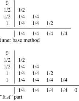
Table 1. RFMSMR(RK2a) – an example for a 2nd order multirate scheme with time step ratioR=2; redundant stages omitted.
0
1 1
1/2 1/2 (RK2a)
0 1/2 1/2 1/2 1/4 1/4
1 1/4 1/4 1/2
1/4 1/4 1/4 1/4 outer base method inner base method
0 1/2 1/2 1/2 1/2 0
1 1 0 0
1 1 0 0 0
1/2 0 0 0 1/2
0 1/2 1/2 1/2 1/4 1/4
1 1/4 1/4 1/2 1 1/4 1/4 1/4 1/4
1/4 1/4 1/4 1/4 0
“slow” part “fast” part
additional order condition is satisfied by the outer method, sO
X i=1
ciO+1−cOi i−1 X j=1
aOi+1,j+ai,jOcOj =1 3.
Third order accuracy in time has been documented by nu-merical tests and has also been proven formally. Order condi-tions for partitioned Runge-Kutta methods can be found for instance in Jackiewicz and Vermiglio (1998).
In order to apply this multirate approach to the advection equation, the advection operator must be split. Commonly a splitting by components is employed. Unfortunately the methods generated via RFSMR generally have unequal sum-mation weightsbfast6=bslow(see Table 1 for an example), so that the methods do not preserve the linear invariants of the system such as the total mass of pollutants. Mass conserva-tion, however, is a strict requirement for atmospheric mod-els. The solution of this problem is to employ a splitting by fluxes. Applied to a decomposition of the domain into slow and fast blocks, flux splitting means that every block com-putes the fluxes leaving its cells. Thus, fast fluxes leaving cells with a stricter local Courant-Friedrichs-Lewy (CFL) re-striction are updated more frequently per macro time step than slow fluxes. As the individual cell outfluxes are com-puted exactly the same way and based on the same concen-tration vector as the corresponding cell influxes, this kind of splitting guarantees mass conservation independent from the partitioned time integration scheme.
3 Implementation details
As the name already suggests the recursive flux splitting mul-tirate algorithm is especially suitable for recursive imple-mentation. This kind of implementation makes it simple to exploit redundancies. The primary aim of multirate meth-ods is to reduce computational cost, usually measured in evaluations of the right-hand side. An objection obvious to
programmers is that the bottleneck in modern hardware is memory access rather than the actual computations on the CPU. This holds the more if a multi-node cluster is employed and data has to be exchanged across the network. Fortunately RFSMR can be implemented with only little memory over-head; additionally communication workload is reduced.
The algorithm is implemented in the multi-scale atmo-spheric chemistry and transport model MUSCAT, (Wolke and Knoth, 2000; Knoth and Wolke, 1998b) developed at the Leibniz Institute for Tropospheric Research in Leipzig. This model is used for scientific process studies as well as online coupled with a meteorological model for several air quality applications in local and regional areas. MUSCAT describes the transport as well as chemical transformations for several gas phase species and particle populations in the atmosphere. The spatial discretisation of the mass balance equations is performed by finite volume techniques on a hi-erarchical grid structure. A second order IMEX scheme is applied for the time integration. The step size control during the implicit integration leads to load imbalances. Therefore, a dynamic workload balancing is implemented (Wolke et al., 2004). This is done using the ParMetis libraries (Karypis et al., 2011; Karypis, 1999). The MUSCAT code is mainly written in FORTRAN90/95 and uses a few additional C li-braries.
This section is organised as follows: first, we shall explain how data is organised in our model, then present the pro-gramme flow of local computations and finally explain data exchange strategies. Since the workload balancing gets more complicated as the programme complexity increases, we will also comment on this issue.
3.1 Data organization and spatial structure
In MUSCAT data is organised hierarchically: the three di-mensional computational domain is decomposed statically into rectangular blocks. This decomposition is applied in
1398 M. Schlegel et al.: Implementation of splitting methods
Table 1.RFMSMR(RK2a) – an example for a 2nd order multirate scheme with time step ratioR= 2; redundant stages omitted.
0 1 1
1/2 1/2 (RK2a)
0 1/2 1/2 1/2 1/4 1/4
1 1/4 1/4 1/2 1/4 1/4 1/4 1/4 outer base method inner base method
0 1/2 1/2 1/2 1/2 0
1 1 0 0
1 1 0 0 0
1/2 0 0 0 1/2
0 1/2 1/2 1/2 1/4 1/4
1 1/4 1/4 1/2 1 1/4 1/4 1/4 1/4
1/4 1/4 1/4 1/4 0 “slow” part “fast” part
naive cells
extended array including halo cells
halo
additional data structure for exchange with...
...northern neighbor
...southern neighbor ...eastern neighbor
...western neighbor
simulation domain
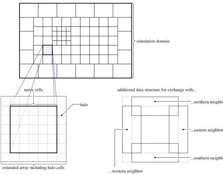
Fig. 1.Illustration of block structure for simulation domain as well as one generic block in MUSCAT.
Fig. 1. Illustration of block structure for simulation domain as well as one generic block in MUSCAT.
horizontal direction only so that every block ranges from ground level through the top of the domain to simulate. An important feature is that each block may have its own spatial refinement level. Thus, selected regions may be examined in more detail. The cell size always is the macro cell size di-vided by an integer power of two. If two blocks are adjacent, their spatial refinement level is allowed to differ by a factor of two maximum. Cell size, adjacency to other blocks, tem-poral refinement level, etc., form the block meta data. Even for parallel processing meta data of all blocks is present on all processors. The main part of the data consists of concen-tration arrays and a number of difference arrays associated with the stage vectors of the employed explicit Runge-Kutta method. Opposed to the meta data, the main data of the block is present only on the processor the block is associated with. Additional variables include geometric data per cell (volume, extend per axis etc.) defined on initialisation and meteorolog-ical data such as wind speed or density of air. The latter may be provided by the COSMO model (Sch¨attler et al., 2011; Steppeler et al., 2003) of the German weather service via on-line coupling or by a simple test driver.
The declaration of the concentration array is done in such a way that cell local values, i.e., the concentrations of the different tracers or species inside of a cell are directly ad-jacent in physical memory. The cell data in turn is organ-ised so that cells within one column (i.e., cells at the same horizontal position) have minimal distance in memory. This layout is advantageous for the computations executed most frequently, i.e., cell local chemistry and column local (verti-cal) diffusion. A number of fully coupled implicit chemistry diffusion steps have to be performed per advection step. This part contributes mainly to the overall computational cost. All arrays have the same shape and dimension making vectorised operations possible.
M. Schlegel et al.: Implementation of splitting methods 1399
neighbouring blocks are needed along the respective bound-aries, see Fig. 1. These data structures correspond to the source termr occurring in Eqs. (4) and (11). Employing a limited third order upwind spatial discretisation (Hundsdor-fer and Verwer, 2003), the halo has to be one cell wide while the additional data structures overlap with the halo cells and the outermost row of actual cells.
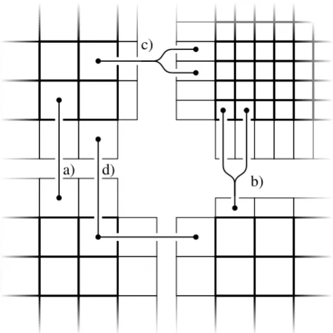
Though the grid of the block is logically cartesian, its geo-metrical interpretation may be different. First of all, the sim-ulation domain usually represents a volume above a spheri-cal surface. Furthermore, perpendicularly to the interface the ghost cells have the extent of the actual cells they overlap with, see Fig. 2. The possible relations between actual cells and ghost cells representing the same physical volume are also marked in Fig. 2. The respective volume may be repre-sented by:
a. one inner cell and one ghost cell,
b. two inner cells and one ghost cell of a coarser neigh-bour,
c. one inner cell and two ghost cells of a finer neighbour or
d. inner cell(s) and ghost cell(s) for each of two neigh-bours.
Case (d) only occurs at block corners and may be compli-cated for neighbour blocks with different spatial refinement levels. These different possible relations have to be taken into account when data is exchanged between blocks.
Keep in mind that the domain is decomposed in the hori-zontal direction only, so that all of the above holds not only for cells in one vertical layer, but also for the columns, rang-ing from the bottom through the top of the simulation do-main.
3.2 Programme flow
In this section we shall discuss the MUSCAT programme flow. For simplicity we shall concentrate on the main inte-gration loop, omitting initialisation, finalisation and output routines. Algorithm (1),...,(6) translates directly into an im-plementation. The following pseudo code evolves all blocks on the given time level fromt0tot0+1t. Here and subse-quently we will employ the terms “time level” and “temporal refinement level” synonymously. In the pseudo code we also shortly write “level”. The macro time step is equivalent to the lowest level.
Table 2.
Examples of two stage, second order explicit Runge-Kutta
methods.
0
1
1
1/2
1/2
0
1/2
1/2
0
1
(RK2a)
(RK2b)
a)
d)
c)
b)
Fig. 2.
Geometrical cell structure of adjacent blocks. Halo cells
depicted with thinner contours. Connectors between blocks indicate
multiple representations of the same physical volume.
stage vectors are only defined for the inner cells. Additional
data structures for the exchange of mass fluxes with
neigh-bor blocks are needed along the respective boundaries, see
Fig. 1. These data structures correspond to the source term
r
occurring in Eq. (4) and (11). Employing a limited third
or-der upwind spatial discretization (Hundsdorfer and Verwer,
2003) the halo has to be one cell wide while the additional
data structures overlap with the halo cells and the outermost
row of actual cells.
Though the grid of the block is logically cartesian, its
geo-metrical interpretation may be different. First of all the
sim-ulation domain usually represents a volume above a
spheri-cal surface. Furthermore perpendicularly to the interface the
ghost cells have the extent of the actual cells they overlap
with, see Fig. 2. The possible relations between actual cells
and ghost cells representing the same physical volume are
also marked in Fig. 2 . The respective volume may be
repre-sented by:
a) one inner cell and one ghost cell,
b) two inner cells and one ghost cell of a coarser neighbor,
c) one inner cell and two ghost cells of a finer neighbor or
d) inner cell(s) and ghost cell(s) for each of two neighbors.
Case d) only occurs at block corners and may be complicated
for neighbor blocks with different spatial refinement levels.
These different possible relations have to be taken into
ac-count when data is exchanged between blocks.
Keep in mind that the domain is decomposed in the
hori-zontal direction only, so that all of the above holds not only
for cells in one vertical layer but also for the columns,
rang-ing from the bottom through the top of the simulation
do-main.
3.2
Program flow
In this section we shall discuss the MUSCAT program
flow.
For simplicity we shall concentrate on the main
integration loop, omitting initialization, finalization and
output routines. Algorithm (1),...,(6) translates directly into
an implementation. The following pseudo code evolves all
blocks on the given time level from
t
0to
t
0+ ∆
t
. Here and
subsequently we will employ the terms “time level” and
“temporal refinement level” synonymously. In the pseudo
code we also shortly write “level”. The macro time step is
equivalent to the lowest level.
1:
procedure
RFSMR (
t
0,
∆
t,
level
)
2:
for
i
= 2
,...,s
+ 1
.
Loop over Runge-Kutta stages
3:
for all
Processor-local blocks
k
do
4:
if
[timelevel of Block
k
]=
level
then
5:
Compute local advective fluxes
f
i−16:
r
:=
P
i−1j=1
(
a
ij−
a
i−1,j)
f
j7:
r
:=
r
+
r
(slow)·
(
c
i−
c
i−1)
8:
exchange
fluxes with neighbor blocks
on same level
r
(equal):=
r
neighbor9:
r
:=
r
+
r
(equal)10:
end
if
11:
end
for
At this point all advective fluxes on time level
level
are
computed and known on all blocks containing the
corre-sponding cell boundary. Note that for exchanges we write
the variables without superscript if the variable is block local
and with a superscript “neighbor” if the variable belongs to
another block. The source term
r
(see line 7) correspond to
the source term
r
ias mathematically defined in Eq. (2). Since
source terms computed during earlier explicit stages are not
needed anymore we employ a single variable. Source terms
r
(slow)computed on a lower time level are defined before
the routine is called. Now a case distinction has to be made,
whether or not the forward step in time associated with the
current Runge–Kutta stage
∆
t
(
c
i−
c
i−1)
is greater than zero.
Fig. 2. Geometrical cell structure of adjacent blocks. Halo cells
de-picted with thinner contours. Connectors between blocks indicate multiple representations of the same physical volume.
1: procedure RFSMR (t0, 1t,level)
2: fori=2, ..., s+1FLoop over Runge-Kutta stages 3: for all Processor-local blockskdo
4: if [timelevel of Blockk]= level then 5: Compute local advective fluxesfi−1
6: r:=Pi−1
j=1(aij−ai−1,j)fj 7: r:=r+r(slow)·(ci−ci−1)
8: exchange fluxes with neighbour blocks on same levelr(equal):=rneighbour 9: r:=r+r(equal)
10: end if
11: end for
At this point, all advective fluxes on time level level are computed and known on all blocks containing the corre-sponding cell boundary. Note that for exchanges we write the variables without superscript if the variable is block lo-cal and with a superscript “neighbour” if the variable belongs to another block. The source termr(see line 7) corresponds to the source termri as mathematically defined in Eq. (2). Since source terms computed during earlier explicit stages are not needed anymore, we employ a single variable. Source termsr(slow)computed on a lower time level are defined be-fore the routine is called. Now a case distinction has to be made, whether or not the forward step in time associated with the current Runge-Kutta stage1t (ci−ci−1)is greater than zero.
12: ifci> ci−1then
13: if there are blocks on a higher level then 14: substeps:= d2(ci−ci−1)e
15: send weighted boundary fluxes to neighbours on higher level:r(neighbourslow) :=r/(ci−ci−1) 16: forl=1, ...,substeps do
17: RFSMR(t0+1t·ci−1+
(l−1)·1t·(ci−ci−1)/substeps, 1t·(ci−ci−1)/substeps, level+1)
18: end for
19: end if
20: for all Processor-local blockskdo 21: if [timelevel of Blockk]= level then 22: DIFFREACT(Y, r, t0+1t·ci−1,
1t·(ci−ci−1))
23: exchange boundary concentration with neighbours on same level
24: end if
25: end for
26: else ifci≤ci−1then
27: for all Processor-local blockskdo 28: if [timelevel of Blockk]= level then
29: Y =Y+1t·r
30: exchange boundary concentration with neighbours on same level
31: send boundary concentration to neighbours on lower level
32: end if
33: end for
34: end if
35: end forFLoop over Runge-Kutta stages 36: end procedure
In this pseudo code we assume that DIFFRE -ACT(Y, r, τ0,1τ) solves the initial value problem given by
c (τ0)=Y, d
dτc=r+F (c, τ ) , τ∈[τ0, τ0+1τ],
withF representing a time dependent diffusion-reaction term and stores the resultc(τ0+1τ )in the variableY.
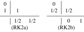
The number of substeps to be taken on the next higher time level can be chosen dynamically in line 14. This allows us to use a different base method in the next level to ensure a time step ratio of 2 between successive time levels. For the method (RK2a) given in Table 2 two substeps will be employed between the first and second stage, while no step will be taken between the second stage and the summation stage; this is equivalent to the formal construction as shown in Table 1. For (RK2b) one step on the next temporal level will be done both for the second stage and the summation stage, again leading to a time step ratio of two. Generally
Table 2. Examples of two stage, second order explicit Runge-Kutta
methods.
0
1 1
1/2 1/2 0 1/2 1/2
0 1
(RK2a) (RK2b)
this time step ratio is possible for any explicit Runge-Kutta method with monotonically increasing nodescsuch that ∀i:ci∈ {0,1/2,1}.
The above synopsis of the actual implementation already shows that due to the recursive calls the programme flow will naturally be structured into multiple phases corresponding to the different time levels. This fact significantly compli-cates balancing. Furthermore, there are different kinds of ex-changes which shall be discussed in the following section. 3.3 Data exchange
In the above listed pseudo code, the following data exchanges are mentioned. Exchanges of fluxes have to be performed be-tween blocks on one level (line 8) or from a lower to a higher time level (line 15). Exchanges of concentrations have to be performed between blocks on a single level (line 23, 30) or from a higher to a lower level (line 31). While the expres-sion “exchange of fluxes” is illustrative it is not exact. Stored and exchanged are not the advective fluxes across cell bound-aries, but the time derivatives of the concentrations per cell computed from the net fluxes. If the boundary fluxes are cast asfi±1/2,jandfi,j±1/2with spatial indexesi, jand cell vol-umeVi,j, then the concentration tendency due to advection reads
d
dtci,j = −
fi+1/2,j−fi−1/2,j+fi,j+1/2−fi,j−1/2 Vi,j
.
Due to the data structure, i.e., the data available for a block and the algorithm employed for the calculation of block lo-cal fluxes, each boundary flux is computed exactly once and sent to the neighbouring block. It is convenient to store the received time derivatives in an additional variable allowing for a distinction between fluxes given by neighbours on the same and on a lower temporal refinement level.
flux
conc. time level0
time level1
flux
flux
conc.
conc. conc. Block 1
Block 2
Block 3
B1
B2
B3 physical domain decomposition
cI1 cI2 cI3 cI4 cI5
cO1 cO2 cO3
cO1 cO2 cO3
Fig. 3.Exchanges in course of a macro time step for method based on RK2a, see also Table 1. ThecOi andcIi denote the nodes of the inner and outer base method.
Considering the geometrical aspects of the various ex-changes it is important to ensure that multiple representations of the same physical volume contain equivalent data. As all exchanged quantities are either cell average values or time derivatives of cell average values this can be accomplished by averaging and constant interpolation of these quantities. We interpret the cell volumesV ⊂Ωas subsets of the simu-lation domainΩ. Further we denote the original quantity and the original volume as given by the sending block with a su-perscript “S” and the copied quantity of the receiving block and the correlated volume with a superscript “R”. The ex-changes for a generic quantityq for different configurations then read:
VS=VR ⇒qR:=qS,
V1S∪V2S=VR ⇒qR:=1 2 q
S 1+qS2
,
VS=V1R∪V2R ⇒q1R=qR2 :=qS,
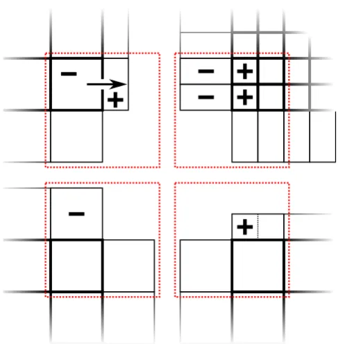
corresponding to the cell relations (a), (b) and (c) as illus-trated in Fig. 2. More complicated relations hold for diago-nal exchanges. For a better understanding see Fig. 4. There a flux across a specific cell boundary is computed from data present in the upper left block. This flux in turn is repre-sented by a source term marked “+” and a sink term marked “–”. As the same physical region is represented 4 times these source and sink terms have to be exchanged to the other
Fig. 4.Multiple representation of the same physical region (marked by red rectangles) and source/sink terms caused by a specific advec-tive flux.
blocks shown. The exchange is complicated by the fact that the source term influences “half a ghost cell” of the lower right block. For this specific configuration this problem can be solved by adding half of the source term to the ghost cell. If as in our implementation the spatial resolution of directly (i.e. not diagonally) adjacent blocks is allowed to differ by a factor of two maximum, nine different configurations of di-agonal overlaps have to be distinguished. Note that didi-agonal exchanges are obsolete if all blocks have the same temporal refinement level, i.e. a classical time integration scheme is employed.
For efficient parallel execution it is desirable to minimize communication cost. Generally it is more efficient to ex-change one big chunk of data instead of several small chunks of equal cumulative size. For this reason inter process change is implemented as a gathering or packing of data, ex-change using MPI routines and finally unpacking of data. As meta data regarding all blocks including adjacency informa-tion is present on all processors every participant of an ex-change knows a priori which data to send and/or to receive. To reduce the amount of data to be exchanged interpolation and averaging is done in such a way that as little data as pos-sible is to be transferred. This means that averaging is done before packing while interpolation is done after unpacking.
3.4 Balancing
If a simulation is to be distributed on multiple cores of one processor, multiple processors or even multiple nodes of a computing cluster, the simulation has to be split in several parts. In the context of air pollution modeling this means a decomposition of the simulation domain into blocks. The available computing elements are then to be assigned to these blocks such that idle times are minimized. For classical time Fig. 3. Exchanges in course of a macro time step for method based
on RK2a, see also Table 1. ThecOi andcIi denote the nodes of the inner and outer base method.
updated from their geometrical counterparts. The rationale for this is that the halo cells of the sending block contain a better approximation than the receiving block’s outer cells. An illustration of the exchanges in the course of one macro time step is given in Fig. 3. The last exchange is necessary to update the higher level block’s outer cells and halo with the result of the correction stage performed on the macro time level.
Considering the geometrical aspects of the various ex-changes, it is important to ensure that multiple representa-tions of the same physical volume contain equivalent data. As all exchanged quantities are either cell average values or time derivatives of cell average values, this can be accomplished by averaging and constant interpolation of these quantities. We interpret the cell volumesV ⊂as subsets of the simu-lation domain. Further we denote the original quantity and the original volume as given by the sending block with a su-perscript “S” and the copied quantity of the receiving block and the correlated volume with a superscript “R”. The ex-changes for a generic quantityq for different configurations then read:
flux
conc.
time level
0
time level
1
flux
flux
conc.
conc. conc.
Block 1
Block 2
Block 3
B1
B2
B3
physical domain
decomposition
c
I1c
I2c
I3c
I4c
I5c
O1c
O 2
c
O 3
c
O1c
O2c
O3Fig. 3.
Exchanges in course of a macro time step for method based
on RK2a, see also Table 1. The
c
Oiand
c
Iidenote the nodes of the
inner and outer base method.
Considering the geometrical aspects of the various
ex-changes it is important to ensure that multiple representations
of the same physical volume contain equivalent data. As all
exchanged quantities are either cell average values or time
derivatives of cell average values this can be accomplished
by averaging and constant interpolation of these quantities.
We interpret the cell volumes
V
⊂
Ω
as subsets of the
simu-lation domain
Ω
. Further we denote the original quantity and
the original volume as given by the sending block with a
su-perscript “S” and the copied quantity of the receiving block
and the correlated volume with a superscript “R”. The
ex-changes for a generic quantity
q
for different configurations
then read:
V
S=
V
R⇒
q
R:=
q
S,
V
1S∪
V
2S=
V
R⇒
q
R:=
1
2
q
S 1
+
q
2S,
V
S=
V
1R∪
V
2R⇒
q
1R=
q
2R:=
q
S,
corresponding to the cell relations (a), (b) and (c) as
illus-trated in Fig. 2. More complicated relations hold for
diago-nal exchanges. For a better understanding see Fig. 4. There
a flux across a specific cell boundary is computed from data
present in the upper left block. This flux in turn is
repre-sented by a source term marked “+” and a sink term marked
“–”. As the same physical region is represented 4 times these
source and sink terms have to be exchanged to the other
Fig. 4.
Multiple representation of the same physical region (marked
by red rectangles) and source/sink terms caused by a specific
advec-tive flux.
blocks shown. The exchange is complicated by the fact that
the source term influences “half a ghost cell” of the lower
right block. For this specific configuration this problem can
be solved by adding half of the source term to the ghost cell.
If as in our implementation the spatial resolution of directly
(i.e. not diagonally) adjacent blocks is allowed to differ by a
factor of two maximum, nine different configurations of
di-agonal overlaps have to be distinguished. Note that didi-agonal
exchanges are obsolete if all blocks have the same temporal
refinement level, i.e. a classical time integration scheme is
employed.
For efficient parallel execution it is desirable to minimize
communication cost. Generally it is more efficient to
ex-change one big chunk of data instead of several small chunks
of equal cumulative size. For this reason inter process
change is implemented as a gathering or packing of data,
ex-change using MPI routines and finally unpacking of data. As
meta data regarding all blocks including adjacency
informa-tion is present on all processors every participant of an
ex-change knows a priori which data to send and/or to receive.
To reduce the amount of data to be exchanged interpolation
and averaging is done in such a way that as little data as
pos-sible is to be transferred. This means that averaging is done
before packing while interpolation is done after unpacking.
3.4
Balancing
If a simulation is to be distributed on multiple cores of one
processor, multiple processors or even multiple nodes of a
computing cluster, the simulation has to be split in several
parts. In the context of air pollution modeling this means
a decomposition of the simulation domain into blocks. The
available computing elements are then to be assigned to these
blocks such that idle times are minimized. For classical time
Fig. 4. Multiple representation of the same physical region (marked
by red rectangles) and source/sink terms caused by a specific advec-tive flux.
VS=VR⇒qR:=qS, V1S∪V2S=VR⇒qR:=1
2
q1S+q2S, VS=V1R∪V2R⇒q1R=q2R:=qS,
corresponding to the cell relations (a), (b) and (c) as illus-trated in Fig. 2. More complicated relations hold for diago-nal exchanges. For a better understanding see Fig. 4. A flux across a specific cell boundary is computed from data present in the upper left block. This flux in turn is represented by a source term marked “+” and a sink term marked “–”. As the same physical region is represented 4 times, these source and sink terms have to be exchanged to the other blocks shown. The exchange is complicated by the fact that the source term influences “half a ghost cell” of the lower right block. For this specific configuration, this problem can be solved by adding half of the source term to the ghost cell. If as in our imple-mentation the spatial resolution of directly (i.e., not diago-nally) adjacent blocks is allowed to differ by a factor of two maximum, nine different configurations of diagonal over-laps have to be distinguished. Note that diagonal exchanges are obsolete if all blocks have the same temporal refinement level, i.e., a classical time integration scheme is employed.
For efficient parallel execution it is desirable to min-imise communication cost. Generally it is more efficient to exchange one big chunk of data instead of several small chunks of equal cumulative size. For this reason inter process
exchange is implemented as a gathering or packing of data, exchange using MPI routines and finally unpacking of data. As meta data regarding all blocks including adjacency infor-mation is present on all processors every participant of an ex-change knows a priori which data to send and/or to receive. To reduce the amount of data to be exchanged interpolation and averaging is done in such a way that as little data as pos-sible is to be transferred. This means that averaging is done before packing while interpolation is done after unpacking. 3.4 Balancing
If a simulation is to be distributed on multiple cores of one processor, multiple processors or even multiple nodes of a computing cluster, the simulation has to be split in several parts. In the context of air pollution modelling this means a decomposition of the simulation domain into blocks. The available computing elements are then to be assigned to these blocks such that idle times are minimised. For classical time integration schemes, this can easily be implemented by per-forming workload balancing. Thus, it can be provided that every processor has approximately the same amount of work to do.
The Metis/ParMetis libraries (Karypis et al., 2011) provide sophisticated balancing algorithms. Balancing problems are interpreted as a class of graph theoretical problems which may be subsumed as “minimise the edge cut without violat-ing node balancviolat-ing constraints”. Blocks of the decomposed simulation domain are mapped to nodes of the graph, nec-essary data exchanges are mapped to the edges connecting these nodes. Consequently minimising the edge cut is equiv-alent to minimising the communication between partitions or processors.
The more complex programme flow in the multirate con-text calls for a more sophisticated approach to balancing. Naive workload balancing is not sufficient to minimise idle times, as the programme flow is structured in multiple phases due to recursive calls, see Fig. 5 for an example. Assuming that the same computational cost is associated with all four mentioned blocks, both presented block distributions are op-timal in the sense of workload balancing. However, the worst case distribution will lead to an unnecessarily high amount of idle times.
Optimally not only the overall workload is balanced, but also the workload for each phase, i.e., for each temporal re-finement level. The Metis/ParMetis libraries offer the possi-bility of multi constraint balancing, (Karypis, 1999). Classi-cal balancing (single constraint) considers one sClassi-calar weight per node and aims at an even distribution of this scalar weight within a margin of tolerance. Opposed to this multi-constraint balancing considers a vector of weights for each node and aims at an even distribution for each vector dimen-sion. For our algorithm that naively means that the weight vectorwfor a block reads
8 M. Schlegel et al.: Implementation of splitting methods
Setup:
– Blocks #1 and #2 on temporal refinement level 0
– Blocks #3 and #4 on temporal refinement level 1.
– Equal workload per block.
block
1
block
2
block
4
processor 1
processor 2
[idle] [idle]
[idle] [idle]
time level 0 1 2,... 1 0
... ... a) Worst case block distribution:
processor 1
processor 2
time level 0 1 1 0
b) Best case block distribution:
block
3
block
4
block
3
block
1
block
2
2,...
... ...
block
1
block
1
block
2
block
2
block
3
block
3
block
4
block
4
Fig. 5. Parallel program flow for different distributions of four blocks on two processors. Thick lines indicate exchanges.
integration schemes this can easily be implemented by per-formingworkload balancing. Thus it can be provided that every processor has approximately the same amount of work to do.
The Metis/ParMetis libraries (Karypis et al., 2003) provide sophisticated balancing algorithms. Balancing problems are interpreted as a class of graph theoretical problems which may be subsumed as “minimize the edge cut without violat-ing node balancviolat-ing constraints”. Blocks of the decomposed simulation domain are mapped to nodes of the graph, nec-essary data exchanges are mapped to the edges connecting these nodes. Consequently minimizing the edge cut is equiv-alent to minimizing the communication between partitions or processors.
The more complex program flow in the multirate context calls for a more sophisticated approach to balancing. Naive workload balancing is not sufficient to minimize idle times, as the program flow is structured in multiple phases due to recursive calls, see Fig. 5 for an example. Assuming that the same computational cost is associated with all four men-tioned blocks, both presented block distributions are optimal in the sense of workload balancing. However the worst case distribution will lead to an unnecessarily high amount of idle times.
Optimally not only the overall workload is balanced but also the workload for each phase, i.e. for each temporal re-finement level. The Metis/ParMetis libraries offer the possi-bility ofmulti constraint balancing, (Karypis, 1999). Classi-cal balancing (single constraint) considers one sClassi-calar weight
straint balancing considers a vector of weights for each node and aims at an even distribution for each vector dimension. For our algorithm that naively means that the weight vector
wfor a block reads
w∈RN, w k=
C ifk=L
0 otherwise,
with N denoting the number of time levels throughout the simulation, Lthe block’s time level and C the number of columns within the block. Choosing this approach will prob-ably not lead to satisfactory results as the constraints leave only little margin for optimization. As a compromise we employ three constraints correlated to the highest temporal refinement level Lmax, the second highest temporal
refine-ment level and the remaining levels. The rationale for this is that in most setups the two highest refinement levels will cause the bigger part of computational cost. Consequently balancing blocks on these levels will lead to an acceptable tradeoff between constraints and idle times. We define the three dimensional weight vector as follows:
w=
(C,0,0) ifL=Lmax
(0,C,0) ifL=Lmax−1 0,0,2LCotherwise
.
The factor 2L in the third case is needed to consider the relative computational cost of blocks on potentially differ-ent time levels. The scaling for the first two compondiffer-ents of the weighting vector is not necessary, as only their relative weights are taken into account by the ParMetis library. To prioritize balancing of the highest temporal refinement levels over the remaining levels, a smaller and thus stricter margin of tolerance is provided for the first component of the weight vector.
Computational tests with realistic scenarios show ambiva-lent results. While multi constraint balancing is suitable to minimize idle times during computation, it generally leads to higher communication cost, as the optimization of commu-nication is hindered by more constraints. Thus it is generally recommendable for such simulations in which local compu-tations take significantly more time than data exchange, e.g. simulations involving computationally expensive chemistry or microphysics. If in contrast to that a simulation is commu-nication dominated, relatively little parallelization speedup can be expected even for optimal distribution of blocks on different processors.
4 Results
The implementation described above was tested with aca-demic and realistic scenarios. Results show good agreement of the solutions obtained with the multirate splitting and clas-sical time integration. We shall present two test cases. The Fig. 5. Parallel programme flow for different distributions of four
blocks on two processors. Thick lines indicate exchanges.
w∈RN, wk=
C ifk=L 0 otherwise ,
withN denoting the number of time levels throughout the simulation, L the block’s time level andC the number of columns within the block. Choosing this approach will prob-ably not lead to satisfactory results as the constraints leave only little margin for optimisation. As a compromise we em-ploy three constraints correlated to the highest temporal re-finement levelLmax, the second highest temporal refinement level and the remaining levels. The rationale for this is that in most setups the two highest refinement levels will cause the bigger part of computational cost. Consequently balanc-ing blocks on these levels will lead to an acceptable tradeoff between constraints and idle times. We define the three di-mensional weight vector as follows:
w=
(C,0,0) ifL=Lmax (0, C,0) ifL=Lmax−1
0,0,2LC
otherwise .
M. Schlegel et al.: Implementation of splitting methods 1403
and a homogeneous, diagonal wind field. The other test case is taken from an earlier study, with a realistic wind field pro-vided by the COSMO model (Hinneburg et al., 2009). Re-sults of the latter case shall demonstrate the potential of mul-tirate schemes for realistic scenarios as well as show remain-ing deficiencies.
4.1 Academic test case
An important characteristic of parallel programs is the speedup1 when solving the problem on multiple proces-sors. For the scenario discussed here we observed not quite an ideal (i.e. linear) speedup, but the overhead is small enough to justify parallel execution. Furthermore due to a sophisticated balancing approach making use of ParMetis’ multi-constraint partitioning capabilities, the parallelization speedup is comparable to the one obtained for the much sim-pler case of singlerate time integration.
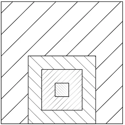
The domain is quadratic in horizontal direction. A com-paratively small region is refined, see Table 3 and Fig. 6. Sources are located within the region most finely resolved.
horizontal relative area number of fraction of
cell size columns cells total
4km ≈69% 3584 ≈18%
2km ≈20% 4096 ≈21%
1km ≈10% 8192 ≈41%
500m ≈1% 4096 ≈21%
Table 3.Synopsis of spatial structure for academic test case.
Fig. 6. Illustration of the spatial structure for academic test run. Hatchings correspond to different grid sizes.
1Not to be confused with the cost reduction due to application
of a multirate scheme.
1/16 1/8 1/4 1/2 1
1 2 4 8 16
simulation
time
/
A
U
number of processors average cost reduction: 48%
singlerate advection multirate advection singlerate adv.-diff.-react. multirate adv.-diff.-react.
Fig. 7. Computational cost for academic test case. The displayed simulation time was normalized such that the singlerate setup on one processor corresponds to unit. Actual computational cost of the pure advection setup is about 1% of the full setup.
In this domain we tested two kinds of model equations: a pure advection with a uniform wind field and advection-diffusion-reaction with the same wind field, vertical diffu-sion and a chemistry model involving point sources in the finest region and 258 different chemical reactions of 98 re-actants. The overall computational cost of the full system is about a factor of 100 larger than that of the pure advection case. These tests are run on different numbers of processors each. We compare the computational cost of the multirate approach to the computational cost without temporal refine-ment, denotedsinglerate. Results are shown in Fig. 7.
As the time step is chosen to be directly proportional to the grid size, the naive cost reduction is approximately 52%. For a pure advection problem we achieve an average multi-rate cost reduction of 59%. Here the exceeding of the naive cost reduction can be explained by reduced communication. The behavior for the full advection-diffusion reaction system however is not intuitive. In the latter case the multirate ap-proach is applied only to the advection operator whose eval-uation contributes about 1 % to the total computational cost. However there still is a significant cost reduction of about 36 %. The reason for this is the behavior of the term solved implicitly depending on the source termr, see Eq. (4). Each update of this source term introduces a discontinuity in the right hand side of the equation. In combination with the error control of the second order implicit solver this causes smaller implicit steps or even makes expensive restarts nec-essary (Knoth and Wolke, 1998a). Fewer updates take place if the outer system is solved using a larger time step, thus indirectly improving the efficiency of the implicit solving.
4.2 Realistic test case
The following test case is taken from a earlier study per-formed by Hinneburg et al. (2009), examining the effects of Fig. 6. Illustration of the spatial structure for academic test run.
Hatchings correspond to different grid sizes.
Table 3. Synopsis of spatial structure for academic test case.
horizontal relative area number of fraction of cell size columns cells total
4 km ≈69 % 3584 ≈18 %
2 km ≈20 % 4096 ≈21 %
1 km ≈10 % 8192 ≈41 %
500 m ≈1 % 4096 ≈21 %
Computational tests with realistic scenarios show ambiva-lent results. While multi-constraint balancing is suitable to minimise idle times during computation, it generally leads to higher communication cost, as the optimisation of communi-cation is hindered by more constraints. Thus, it is generally recommendable for such simulations in which local compu-tations take significantly more time than data exchange, e.g., simulations involving computationally expensive chemistry or microphysics. If in contrast to that a simulation is commu-nication dominated, relatively little parallelisation speedup can be expected even for optimal distribution of blocks on different processors.
4 Results
The implementation described above was tested with aca-demic and realistic scenarios. Results show good agreement of the solutions obtained with the multirate splitting and clas-sical time integration. We shall present two test cases. The first test is designed to make optimal use of the multirate ap-proach by employing a grid with a small region of interest and a homogeneous, diagonal wind field. The other test case
M. Schlegel et al.: Implementation of splitting methods 9
and a homogeneous, diagonal wind field. The other test case is taken from an earlier study, with a realistic wind field pro-vided by the COSMO model (Hinneburg et al., 2009). Re-sults of the latter case shall demonstrate the potential of mul-tirate schemes for realistic scenarios as well as show remain-ing deficiencies.
4.1 Academic test case
An important characteristic of parallel programs is the speedup1 when solving the problem on multiple
proces-sors. For the scenario discussed here we observed not quite an ideal (i.e. linear) speedup, but the overhead is small enough to justify parallel execution. Furthermore due to a sophisticated balancing approach making use of ParMetis’ multi-constraint partitioning capabilities, the parallelization speedup is comparable to the one obtained for the much sim-pler case of singlerate time integration.
The domain is quadratic in horizontal direction. A com-paratively small region is refined, see Table 3 and Fig. 6. Sources are located within the region most finely resolved.
horizontal relative area number of fraction of cell size columns cells total 4km ≈69% 3584 ≈18% 2km ≈20% 4096 ≈21% 1km ≈10% 8192 ≈41%
500m ≈1% 4096 ≈21%
Table 3.Synopsis of spatial structure for academic test case.
Fig. 6. Illustration of the spatial structure for academic test run. Hatchings correspond to different grid sizes.
1
Not to be confused with the cost reduction due to application of a multirate scheme.
1/16 1/8 1/4 1/2 1
1 2 4 8 16
simulation
time
/
A
U
number of processors average cost reduction: 48%
singlerate advection multirate advection singlerate adv.-diff.-react. multirate adv.-diff.-react.
Fig. 7. Computational cost for academic test case. The displayed simulation time was normalized such that the singlerate setup on one processor corresponds to unit. Actual computational cost of the pure advection setup is about 1% of the full setup.
In this domain we tested two kinds of model equations: a pure advection with a uniform wind field and advection-diffusion-reaction with the same wind field, vertical diffu-sion and a chemistry model involving point sources in the finest region and 258 different chemical reactions of 98 re-actants. The overall computational cost of the full system is about a factor of 100 larger than that of the pure advection case. These tests are run on different numbers of processors each. We compare the computational cost of the multirate approach to the computational cost without temporal refine-ment, denotedsinglerate. Results are shown in Fig. 7.
As the time step is chosen to be directly proportional to the grid size, the naive cost reduction is approximately 52%. For a pure advection problem we achieve an average multi-rate cost reduction of 59%. Here the exceeding of the naive cost reduction can be explained by reduced communication. The behavior for the full advection-diffusion reaction system however is not intuitive. In the latter case the multirate ap-proach is applied only to the advection operator whose eval-uation contributes about 1 % to the total computational cost. However there still is a significant cost reduction of about 36 %. The reason for this is the behavior of the term solved implicitly depending on the source termr, see Eq. (4). Each update of this source term introduces a discontinuity in the right hand side of the equation. In combination with the error control of the second order implicit solver this causes smaller implicit steps or even makes expensive restarts nec-essary (Knoth and Wolke, 1998a). Fewer updates take place if the outer system is solved using a larger time step, thus indirectly improving the efficiency of the implicit solving.
4.2 Realistic test case
The following test case is taken from a earlier study per-formed by Hinneburg et al. (2009), examining the effects of
Fig. 7. Computational cost for academic test case. The displayed
simulation time was normalised such that the single-rate setup on one processor corresponds to unit. Actual computational cost of the pure advection setup is about 1 % of the full setup.
is taken from an earlier study, with a realistic wind field pro-vided by the COSMO model (Hinneburg et al., 2009). Re-sults of the latter case shall demonstrate the potential of mul-tirate schemes for realistic scenarios as well as show remain-ing deficiencies.
4.1 Academic test case
An important characteristic of parallel programmes is the speedup1 when solving the problem on multiple proces-sors. For the scenario discussed here we observed not quite an ideal (i.e., linear) speedup, but the overhead is small enough to justify parallel execution. Furthermore, due to a sophisticated balancing approach making use of ParMetis’ multi-constraint partitioning capabilities, the parallelisation speedup is comparable to the one obtained for the much sim-pler case of single-rate time integration.
The domain is quadratic in horizontal direction. A compar-atively small region is refined, see Table 3 and Fig. 6. Sources are located within the region most finely resolved.
In this domain, we tested two kinds of model equations: a pure advection with a uniform wind field and advection-diffusion-reaction with the same wind field, vertical diffu-sion and a chemistry model involving point sources in the finest region and 258 different chemical reactions of 98 re-actants. The overall computational cost of the full system is about a factor of 100 larger than that of the pure advection case. These tests are run on different numbers of processors each. We compare the computational cost of the multirate approach to the computational cost without temporal refine-ment, denoted single-rate. Results are shown in Fig. 7.
As the time step is chosen to be directly proportional to the grid size, the naive cost reduction is approximately 52 %. 1Not to be confused with the cost reduction due to application of a multirate scheme.
1404 M. Schlegel et al.: Implementation of splitting methods
emissions of two power plants in Germany. One plant is
lo-cated near Lippendorf, the other near Boxberg, both in the
federal country Saxony. Emissions are modeled by point
sources which for the larger part represent the chimneys of
the power plants, and area sources representing the emissions
according to land usage. Meteorological data is provided by
the COSMO model via online coupling.
horizontal
relative area
number of
fraction of
cell size
columns
cells total
2.8km
≈
41.0%
1748
≈
7.3%
1.4km
≈
41.0%
6992
≈
29.2%
700m
≈
16.6%
11312
≈
47.2%
350m
≈
1.4%
3904
≈
16.3%
Table 4.
Synopsis of spatial structure for realistic test case.
Fig. 8.
Illustration of the spatial structure for realistic test run.
Hatchings correspond to different grid sizes.
1/8
1/4
1/2
1
1
2
4
8
16
simulation
time
/
A
U
number of processors
average cost reduction: 29%
singlerate
multirate
Fig. 9.
Computational cost for realistic test case. The displayed
simulation time was normalized such that the singlerate setup on
one processor corresponds to unit.
Again we employ a grid with four levels of refinement with
small, highly resolved regions around the power plants,
to-talling about 1 % of the overall area, see Table 4 and Fig. 8.
The high resolution in this context is chosen to ensure an
accurate description of the near field chemistry around the
power plants by reducing numerical diffusion. Exactly equal
parts of the total area are on the coarsest and second coarsest
refinement level. Chemical reactions are modeled as in the
more complex of the academic test cases with 258 different
chemical reactions of 98 reactants.
Assuming a homogeneous wind field we would expect a
slightly higher reduction of computational cost as for the
academic test case with equal diffusion-reaction setup, as
a smaller fraction of cells is on the finest refinement level.
The actually obtained cost reduction is lower, see also Fig. 9.
This results from the fact that the wind fields provided by
the COSMO model exhibit strong variability in all of the
computational domain. A more sophisticated time step
se-lection based on the characteristic times of the individual
blocks rather than based solely on the spatial resolution can
be constructed with relative ease. Complications arise for
parallel execution – if the temporal refinement level of a
block is changed, a redistribution of the blocks is necessary.
This holds for either of the balancing approaches discussed
in Sect. 3.4.
A further defect concerns the parallelization speedup:
while the problem scales well for up to eight processors,
em-ploying sixteen processors yields only very little
improve-ment. At least in part this results from inhomogeneities due
to the distribution of the point sources. The strongest point
sources are inhomogeneously distributed on the blocks with
the highest temporal and spatial refinement level. Each of
the point sources induces significantly increased cost for the
chemistry solver. For up to eight processors the blocks
con-taining the point sources are distributed evenly on all
proces-sors; for more processors this is not the case. This problem is
even more complicated due to the temporally varying wind
field. Due to higher concentrations the speed of chemical
re-actions inside of the plume is significantly higher than in free
air. If the plume is transported into a previously empty cell,
computational cost of this cell is increased for the next time
step. This effect can not easily be taken into consideration
a priori. However employing dynamic repartitioning based
on the measured workload per block seems to be a promising
way to tackle this problem.
Since the correction of both of the mentioned defects
in-volves the implementation of a complex repartitioning
rou-tine it seems recommendable to implement a conjunctive
so-lution.
5
Conclusions
In this paper we presented details on an efficient
implemen-tation of a general splitting approach. This approach is
em-ployed to obtain a multirate-IMEX splitting, i.e. advection
for different physical domains is solved with different
ex-plicit time steps depending on the grid size while
diffusion-reaction equations are solved implicitly. We have shown that
the presented implementation is efficient in the sense that
Fig. 8. Illustration of the spatial structure for realistic test run.
Hatchings correspond to different grid sizes.
For a pure advection problem, we achieve an average multi-rate cost reduction of 59 %. Here the exceeding of the naive cost reduction can be explained by reduced communication. The behaviour for the full advection-diffusion reaction sys-tem, however, is not intuitive. In the latter case, the multirate approach is applied only to the advection operator whose evaluation contributes about 1 % to the total computational cost. However, there still is a significant cost reduction of about 36 %. The reason for this is the behaviour of the term solved implicitly depending on the source termr, see Eq. (4). Each update of this source term introduces a discontinuity in the right-hand side of the equation. In combination with the error control of the second order implicit solver this causes smaller implicit steps or even makes expensive restarts nec-essary (Knoth and Wolke, 1998a). Fewer updates take place if the outer system is solved using a larger time step, thus, indirectly improving the efficiency of the implicit solving. 4.2 Realistic test case
The following test case is taken from a earlier study per-formed by Hinneburg et al. (2009), examining the effects of emissions of two power plants in Germany. One plant is lo-cated near Lippendorf, the other near Boxberg, both in the federal country Saxony. Emissions are modelled by point sources which for the larger part represent the chimneys of the power plants, and area sources representing the emissions according to land usage. Meteorological data is provided by the COSMO model via online coupling.
Again we employ a grid with four levels of refinement with small, highly resolved regions around the power plants, to-talling about 1 % of the overall area, see Table 4 and Fig. 8. The high resolution in this context is chosen to ensure an accurate description of the near field chemistry around the power plants by reducing numerical diffusion. Exactly equal parts of the total area are on the coarsest and second coarsest
Table 4. Synopsis of spatial structure for realistic test case.
horizontal relative area number of fraction of cell size columns cells total
2.8 km ≈41.0 % 1748 ≈7.3 %
1.4 km ≈41.0 % 6992 ≈29.2 %
700 m ≈16.6 % 11312 ≈47.2 %
350 m ≈1.4 % 3904 ≈16.3 %
emissions of two power plants in Germany. One plant is lo-cated near Lippendorf, the other near Boxberg, both in the federal country Saxony. Emissions are modeled by point sources which for the larger part represent the chimneys of the power plants, and area sources representing the emissions according to land usage. Meteorological data is provided by the COSMO model via online coupling.
horizontal relative area number of fraction of cell size columns cells total 2.8km ≈41.0% 1748 ≈7.3% 1.4km ≈41.0% 6992 ≈29.2% 700m ≈16.6% 11312 ≈47.2% 350m ≈1.4% 3904 ≈16.3%
Table 4.Synopsis of spatial structure for realistic test case.
Fig. 8. Illustration of the spatial structure for realistic test run. Hatchings correspond to different grid sizes.
1/8 1/4 1/2 1
1 2 4 8 16
simulation
time
/
A
U
number of processors average cost reduction: 29%
singlerate multirate
Fig. 9. Computational cost for realistic test case. The displayed simulation time was normalized such that the singlerate setup on one processor corresponds to unit.
Again we employ a grid with four levels of refinement with small, highly resolved regions around the power plants, to-talling about 1 % of the overall area, see Table 4 and Fig. 8. The high resolution in this context is chosen to ensure an accurate description of the near field chemistry around the
power plants by reducing numerical diffusion. Exactly equal parts of the total area are on the coarsest and second coarsest refinement level. Chemical reactions are modeled as in the more complex of the academic test cases with 258 different chemical reactions of 98 reactants.
Assuming a homogeneous wind field we would expect a slightly higher reduction of computational cost as for the academic test case with equal diffusion-reaction setup, as a smaller fraction of cells is on the finest refinement level. The actually obtained cost reduction is lower, see also Fig. 9. This results from the fact that the wind fields provided by the COSMO model exhibit strong variability in all of the computational domain. A more sophisticated time step se-lection based on the characteristic times of the individual blocks rather than based solely on the spatial resolution can be constructed with relative ease. Complications arise for parallel execution – if the temporal refinement level of a block is changed, a redistribution of the blocks is necessary. This holds for either of the balancing approaches discussed in Sect. 3.4.
A further defect concerns the parallelization speedup: while the problem scales well for up to eight processors, em-ploying sixteen processors yields only very little improve-ment. At least in part this results from inhomogeneities due to the distribution of the point sources. The strongest point sources are inhomogeneously distributed on the blocks with the highest temporal and spatial refinement level. Each of the point sources induces significantly increased cost for the chemistry solver. For up to eight processors the blocks con-taining the point sources are distributed evenly on all proces-sors; for more processors this is not the case. This problem is even more complicated due to the temporally varying wind field. Due to higher concentrations the speed of chemical re-actions inside of the plume is significantly higher than in free air. If the plume is transported into a previously empty cell, computational cost of this cell is increased for the next time step. This effect can not easily be taken into consideration a priori. However employing dynamic repartitioning based on the measured workload per block seems to be a promising way to tackle this problem.
Since the correction of both of the mentioned defects in-volves the implementation of a complex repartitioning rou-tine it seems recommendable to implement a conjunctive so-lution.
5 Conclusions
In this paper we presented details on an efficient implemen-tation of a general splitting approach. This approach is em-ployed to obtain a multirate-IMEX splitting, i.e. advection for different physical domains is solved with different ex-plicit time steps depending on the grid size while diffusion-reaction equations are solved implicitly. We have shown that the presented implementation is efficient in the sense that
Fig. 9. Computational cost for realistic test case. The displayed
sim-ulation time was normalised such that the single-rate setup on one processor corresponds to unit.
refinement level. Chemical reactions are modelled as in the more complex of the academic test cases with 258 different chemical reactions of 98 reactants.
Assuming a homogeneous wind field we would expect a slightly higher reduction of computational cost as for the academic test case with equal diffusion-reaction setup, as a smaller fraction of cells is on the finest refinement level. The actually obtained cost reduction is lower, see also Fig. 9. This results from the fact that the wind fields provided by the COSMO model exhibit strong variability in all of the computational domain. A more sophisticated time step selec-tion based on the characteristic times of the individual blocks rather than based solely on the spatial resolution can be con-structed with relative ease. Complications arise for paral-lel execution – if the temporal refinement level of a block is changed, a redistribution of the blocks is necessary. This holds for either of the balancing approaches discussed in Sect. 3.4.