www.geosci-model-dev.net/9/2833/2016/ doi:10.5194/gmd-9-2833-2016
© Author(s) 2016. CC Attribution 3.0 License.
Land-surface parameter optimisation using data assimilation
techniques: the adJULES system V1.0
Nina M. Raoult, Tim E. Jupp, Peter M. Cox, and Catherine M. Luke
National Centre for Earth Observation, University of Exeter, Exeter EX4 4QF, UK Correspondence to:Nina M. Raoult ([email protected])
Received: 29 December 2015 – Published in Geosci. Model Dev. Discuss.: 20 January 2016 Revised: 11 July 2016 – Accepted: 19 July 2016 – Published: 25 August 2016
Abstract. Land-surface models (LSMs) are crucial com-ponents of the Earth system models (ESMs) that are used to make coupled climate–carbon cycle projections for the 21st century. The Joint UK Land Environment Simulator (JULES) is the land-surface model used in the climate and weather forecast models of the UK Met Office. JULES is also extensively used offline as a land-surface impacts tool, forced with climatologies into the future. In this study, JULES is automatically differentiated with respect to JULES param-eters using commercial software from FastOpt, resulting in an analytical gradient, or adjoint, of the model. Using this adjoint, the adJULES parameter estimation system has been developed to search for locally optimum parameters by cali-brating against observations. This paper describes adJULES in a data assimilation framework and demonstrates its ability to improve the model–data fit using eddy-covariance mea-surements of gross primary production (GPP) and latent heat (LE) fluxes. adJULES also has the ability to calibrate over multiple sites simultaneously. This feature is used to define new optimised parameter values for the five plant functional types (PFTs) in JULES. The optimised PFT-specific param-eters improve the performance of JULES at over 85 % of the sites used in the study, at both the calibration and eval-uation stages. The new improved parameters for JULES are presented along with the associated uncertainties for each pa-rameter.
1 Introduction
Land-surface models (LSMs) have formed an important component of climate models for many decades now (Pit-man, 2003). First generation land-surface schemes focussed
on providing the lower boundary condition for atmospheric models by calculating the land–atmosphere fluxes of heat, moisture, and momentum, and updating the surface state variables on which these fluxes depend (e.g. soil tempera-ture, soil moistempera-ture, snow cover). In the mid- to late 1990s some land-surface modelling groups began to introduce ad-ditional aspects of biology into their schemes, most notably the dynamic control of transpiration by leaf stomata and the connected rates of leaf photosynthesis (Sellers et al., 1997; Cox et al., 1999).
In the early 2000s, climate modelling groups began to use the carbon fluxes simulated by LSMs within first generation climate–carbon cycle models (Cox et al., 2000; Friedling-stein et al., 2001). These early results, and a subsequent model inter-comparison (Friedlingstein et al., 2006), high-lighted the uncertainties associated with land carbon–climate feedbacks. The 5th Assessment Report of the Intergovern-mental Panel on Climate Change (IPCC AR5; Stocker et al., 2013) for the first time routinely included models with an in-teractive carbon cycle (now called Earth system models or ESMs), confirming that land responses to climate and CO2 are amongst the largest of the uncertainties in future climate change projections (Arora and Boer, 2005; Brovkin et al., 2013; Jones et al., 2013; Friedlingstein et al., 2013). Any fu-ture decreased ability of the land surface to drawdown atmo-spheric CO2could imply smaller “compatible emissions” in order to stay below key warming thresholds such as 2◦.
misrep-resentation of land-surface processes and also the neglect of important processes (such as nitrogen limitations on plant growth, see for example Thornton et al., 2007; Zaehle et al., 2010), or canopy light interception (Mercado et al., 2009). The drive to reduce process uncertainty almost invariably leads to increases in LSM complexity, which typically leads to the introduction of additional internal model parameters. Parameter uncertainty arises from uncertainty in these inter-nal model parameters. The evolution of LSMs has therefore involved an attempt to reduce process uncertainty by increas-ing model realism/complexity, but at the cost of increasincreas-ing parameter uncertainty. This paper concerns the development and application of a technique to reduce parameter uncer-tainty in the widely used Joint UK Land Environment Simu-lator (JULES) LSM (Best et al., 2011; Clark et al., 2011).
Optimisation techniques come under the umbrella of model–data fusion and range from simple ad hoc parame-ter tuning to rigorous data assimilation frameworks. These approaches have been used in a number of studies, covering various LSMs, to derive vectors of parameters that improve model–data fit significantly (e.g. Wang et al., 2001, 2007; Re-ichstein et al., 2003; Knorr and Kattge, 2005; Raupach et al., 2005; Santaren et al., 2007; Thum et al., 2008; Williams et al., 2009; Peng et al., 2011). Many of these studies cali-brate the model at individual measurement sites. Given the small spatial footprint of each flux tower, this can often re-sult in over-tuning. This over-tuning may occur when a single site does not represent the full range of a plant functional type (PFT), given different tree types, tree ages, and above-ground biomass found at each site. There may be some anomalous plants in the small footprint that are not representative of the PFTs over a broader area. The optimised model parameters are site specific and often struggle to perform as well when generalised over other sites (Xiao et al., 2011).
The majority of LSMs group vegetation into a small num-ber of PFTs. Model parameters are assumed to be generic over each PFT. Through different optimisation techniques, some studies have tried to assess the robustness of PFT-specific parameters (e.g. Kuppel et al., 2014). Medvigy et al. (2009) and Verbeeck et al. (2011) both showed that param-eters derived at one site can perform well on a similar site and over the surrounding region (Medvigy and Moorcroft, 2011). However, a contradictory study by Groenendijk et al. (2010) found that there was cross-site parameter variability after optimisation within the PFT groupings.
In the last few years, there has been a move towards deriv-ing PFT-specific parameters usderiv-ing data from multiple sites, the results of which have been generally positive (e.g. Xiao et al., 2011 and Kuppel et al., 2012). Both of these studies used data from multiple sites in their optimisation (calling it multi-site optimisation) and have commented on the robust-ness of this technique, showing that the choice of the initial parameter vector had little effect on the optimised values.
Kuppel et al. (2012) compared different approaches for finding generic PFT-specific parameters, such as averaging
optimised parameter vectors over PFTs and directly optimis-ing over multiple sites. They found that the latter method was best for finding PFT-specific parameters. The multi-site op-timisation procedure was refined in Kuppel et al. (2014), ex-tended to other PFTs, and evaluated at a global scale.
For global modelling, there is a clear need to find generic parameters and associated uncertainties for each PFT, by op-timising against observations in a reproducible way. This paper presents a model–data fusion framework, called ad-JULES, that allows data from multiple sites to be used si-multaneously in order to improve the JULES land-surface model. The adJULES system uses the adjoint method, which finds minima rapidly across multiple parameters via matrix inversion and has the advantage of reproducibility. Replicat-ing these findReplicat-ings usReplicat-ing brute-force optimisation would be prohibitively expensive computationally.
This paper aims to answer the following questions: – Can a (locally) optimum vector of generic parameters
for each of the JULES PFT classes be found?
– How does the optimal PFT parameter vector compare to parameter vectors found by optimising each site indi-vidually?
– How robust is the adJULES system when optimising over multiple sites?
– What uncertainty is associated with each parameter? In Sect. 2, methods and data used in the study are de-scribed. The JULES land-surface model and our new data assimilation system (adJULES), are introduced, along with the data used and the parameters chosen to be optimised in the study. In Sect. 3, the results are presented. The methodol-ogy for optimising over multiple sites simultaneously is val-idated, and optimum parameter values are provided for each JULES PFT. The performance of the new parameter sets is assessed and shown to significantly improve the fit of the JULES model to the observations. The conclusions are laid out in Sect. 4.
2 Methods and data
2.1 The JULES land-surface model
The JULES land-surface model (Best et al., 2011; Clark et al., 2011) simulates the interactions between the land and the atmosphere. Originally developed from the Met Of-fice Surface Exchange Scheme (MOSES) (Cox et al., 1999), JULES can be used “offline” with observed atmospheric forcing data, or can be coupled into a global circulation model (GCM). JULES is the land-surface model used in the UK Met Office Unified Model.
Table 1.Parameters in optimisation vector, with descriptions.
Symbol Name in code Description Units
n0 nl0 Top leaf nitrogen concentration kg N (kg C)−1
f0 f0 Maximum ratio of internal to external CO2 –
dr rootd_ft Root depth m
α alpha Quantum efficiency mol CO2per mol PAR photons δc
δl dcatch_dlai Rate of change of canopy interception capacity with LAI (leaf area index) kg m −2
Tlow tlow Lower temperature for photosynthesis ◦C
Tupp tupp Upper temperature for photosynthesis ◦C
dqc dqcrit Humidity deficit at which stomata close kg kg−1
to time series of the state of the overlying atmosphere (Best et al., 2011; Clark et al., 2011). Processes such as evapora-tion, plant growth, and soil microbial activity are all linked through mathematical equations that quantify how environ-mental conditions affect evapotranspiration, heat balance, respiration, photosynthesis, and carbon assimilation (Best et al., 2011; Clark et al., 2011). JULES runs at a given sub-daily step (typically 30 min), using meteorological drivers of rainfall, incoming radiation, temperature, humidity, and wind speed as inputs.
Vegetation in the JULES model is categorised into five PFTs: broadleaf trees (BT), needleleaf trees (NT), C3 grasses (C3G), C4 grasses (C4G), and shrubs (Sh). Default parame-ters for these PFT classes are taken from a previous study (Blyth et al., 2010).
The eight parameters that are calibrated within this study (see Table 1) relate predominantly to leaf-level stomatal con-ductance (g) and photosynthesis (A). Four of these parame-ters control the responses ofgandAto environmental con-ditions such as surface temperature (Tupp,Tlow), solar radia-tion (α), and atmospheric humidity deficit (dqc). Two other calibration parameters (f0,nl0) essentially control the max-imum values ofgandA. The remaining two calibration pa-rameters influence the hydrological partitioning at the land surface and relate to the amount of rainfall intercepted by the plant canopy (δc/δL), and the “root depth” (dr) from which each PFT can access soil water for transpiration. The sim-ulated latent heat flux and gross primary productivity have been found to be especially sensitive to these parameters in previous studies (Blyth et al., 2010).
The full set of equations within the JULES model is doc-umented in the literature by Best et al. (2011) and Clark et al. (2011), but the key equations are highlighted below. In JULES, leaf-level photosynthesis and stomatal conductance are treated with a coupled model (Cox et al., 1998). Based on the models of Collatz et al. (1991, 1992), leaf-level pho-tosynthesisAis controlled by the carboxylation rate (which depends onn0,Tlow,Tupp) and light-limited photosynthesis (which depends onα). It follows that
A=A(n0, α, Tlow, Tupp, ci, β), (1)
whereci is the internal CO2 concentration inside the leaf, andβ is a soil moisture stress factor, which depends on the vertical soil moisture profileθ, and the plant root depthdr:
β=β(θ, dr). (2)
The internal CO2 concentrationci is assumed to be depen-dent on the external CO2 concentration ca and the atmo-spheric humidity deficitδq(Cox et al., 1998) via the equation
ci−c∗
ca−c∗
=f0
1− δq
δqc
, (3)
wherec∗is the CO2compensation point, andf0andδqcare parameters that are calibrated in this study. The stomatal con-ductance for water vapourgis diagnosed in JULES from the leaf-level photosynthesisAand the internal and external CO2 concentrations:
g=1.6 A ca−ci
. (4)
The factor of 1.6 converts the stomatal conductance for CO2 into a stomatal conductance for water vapour. The scaling-up from leaf to canopy level in this version of JULES uses a “big-leaf” approach (Cox et al., 1999).
2.2 Data assimilation system
similar in these two applications of data assimilation. This paper is certainly not the first to define parameter estima-tion of this form as data assimilaestima-tion (Braswell et al., 2005; Stöckli et al., 2008; Verbeeck et al., 2011; Kuppel et al., 2012; Hararuk et al., 2014), but the reader should note the subtle difference between our definition of data assimilation and that commonly used in weather forecasting.
Even a relatively simplistic land-surface representation such as JULES has over a hundred internal parameters representing the environmental sensitivities of the various land-surface types and PFTs within the model. In general these parameters are chosen to represent measurable “real-world” quantities (e.g. aerodynamic roughness length, sur-face albedo, plant root depth). This allows for observation-ally based estimates of these parameters to be made in the early stages of the model development process. However, the detailed performance of a land-surface model can be very sensitive to such internal parameters. It is therefore common for land-surface modellers to calibrate their models against available observations, such as eddy-covariance flux data. This is typically carried out in a rather ad hoc manner with the modeller varying the parameters that he/she believes are most relevant to the model performance. Such model tuning is by its very nature subjective, lacks reproducibility, and is often sub-optimal because the modeller is unable to explore the full feasible parameter space through such a manual tech-nique.
This paper describes a more objective approach to land-surface model calibration, adopting ideas from the applied mathematics of data assimilation as used widely in weather forecasting and other disciplines, and motivated by pioneer-ing attempts at carbon cycle data assimilation (Rayner et al., 2005; Kaminski et al., 2013). It utilises the adjoint of the JULES model, derived by automatic differentiation, which enables efficient and objective calibration against observa-tions. Importantly, adJULES also allows the uncertainties in the best-fit parameters to be estimated. Such uncertainties are important information for model users, and can also form the basis for observation-constrained estimates of posterior probability density functions for the land-surface parameter perturbations used in climate model ensembles (e.g. Booth et al., 2012).
2.2.1 The theory of adJULES
JULES generates a modelled time series for a given vector of internal parameters, z. The cost function, f (z), consists of a weighted sum of squares of the difference between mt (the vector of model outputs at timet), andot (the vector of observations at timet), combined with a term quadratic in the difference between parameter valueszand initial parameter valuesz0:
f (z; ˆz,z0)=1
2
hX
t
(mt(z)−ot)TR(zˆ)−1(mt(z)−ot)
+λ(z−z0)TB−1(z−z0)
i
. (5)
Here,R(zˆ)=1
n
Pn
t=1(m(zˆ)t−ot)(m(zˆ)t−ot)T denotes the error cross-product matrix produced by a JULES run with a parameter valuezˆ. In an optimisation, zandzˆ are updated separately in nested loops, having both been initialised to the default JULES parameter valuez0. In the inner loop, z is varied to minimise the cost function (termination criterion:
∇f ≈0) for the current value of zˆ. In the outer loop,zˆ is reset to the new value ofzfrom the inner loop (termination criterion: change inzˆnegligible). At the end of an optimisa-tion, therefore, the matrixRconveys information about the error correlation structure in a JULES run with optimal pa-rameter values.
The matrixBdescribes the prior covariances assigned to the parameters, and is here chosen to be a diagonal ma-trix proportional to the inverse square of the ranges allowed for each parameter. The prior uncertainties are therefore as-sumed to be uncorrelated between the parameters. The con-stant of proportionalityλcontrols the relative importance of the background term (i.e. the right-hand term in Eq. 5) and the error term (i.e. the left-hand term in Eq. 5). Larger values ofλhelp condition the problem and force parameter values to be close to the initial valuez0(Bouttier and Courtier, 1999). All parameters and observations are equally weighted in this cost function.
The optimal vector of parameters is the vectorzthat min-imises the cost function (Eq. 5). The aim of adJULES is to find this vector. adJULES minimises the cost function itera-tively using the gradient descent algorithm L-BFGS-B (Byrd et al., 1995, optim: R Development Core Team, 2015). This algorithm is based on the BFGS quasi-Newton method but is modified to use limited memory, for computational afford-ability, and box constraints, so each parameter is given an upper and lower bound based on expert opinion or on physi-cal reasoning (Byrd et al., 1995).
At each iteration, the gradient∇f (z)of the cost function f (z)is computed with respect to all parameters, using the adjoint model of JULES. The adjoint is generated with the automatic differentiator tool TAF (Transformation of Algo-rithms in Fortran; see Giering et al., 2005). Automatic differ-entiation relies on using the chain rule; the choice of forward or reverse mode refers to the order in which the derivatives are computed. Calculating∇f (z)is most efficient in reverse mode as only one sweep is needed to generate the deriva-tive with respect to all parameters (Bartholomew-Biggs et al., 2000).
Meteorological data Parameters
Modelled time series
JULES z0= (z1, z2, ..., zn)T0
t
t
Observed time series
b
b
b b b
t
Cost
f(z) adjoint
∇f(z)
BFGS Optimal?
N
Y
New parameters
z= (z1, z2, ..., zn)T
Optimised time series
t
Optimal parameters
z1= (z1, z2, ..., zn)T1
Hessian to give uncertainty bounds
∂2f
∂zi∂zj
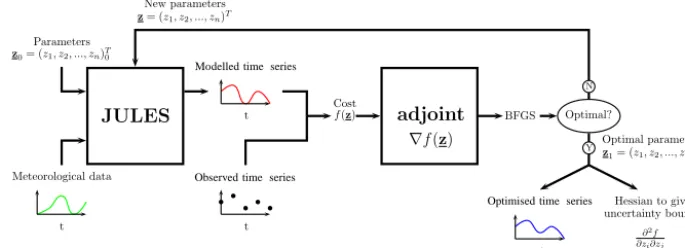
Figure 1. Schematic of the adJULES parameter estimation system starting with the initial parameter vectorz0. This is usually based on
default JULES parameter values (Blyth et al., 2010). The optimised parameter vector is denotedz1.
then repeated, the locally optimised parameters are fed back through JULES, generating a new modelled time series and hence a new cost function. The loop terminates when the modelled time series no longer improves (Fig. 1).
2.2.2 Multi-site implementation
In its simplest form, adJULES runs at a single grid-point lo-cation and so the derived optimal parameter vector is site spe-cific. On the other hand, multi-site optimisation aims to find values for a common set of parameters, using data from mul-tiple locations. The definition of the cost function (Eq. 5) can be extended to include the observations from allSsites, and its derivative found in order to use the L-BFGS-B algorithm again. The extended cost function is the sum of the individual cost functions for each sites. Similarly, the first and second derivatives of this new cost function can be defined using the sum of the derivatives at the individual sites.
f (z; ˆz,z0)= 1 2
hX
s
X
t
(mt,s(z)−ot,s)TRs(zˆ)−1
(mt,s(z)−ot,s)+Sλ(z−z0)TB−1(z−z0)
i
(6) An additive cost function, where the optimisation criterion is to minimise the total cost, was chosen over a cost func-tion where all individual cost funcfunc-tions are required to be improve. All of the sites were used in finding the optimal pa-rameter vector for each PFT, so that sites that do not improve with the rest of the PFT suggest incorrect classification of the site or issues with the PFT definitions.
2.3 Eddy-covariance flux data
The eddy-covariance flux data used in this study are part of FLUXNET (Baldocchi et al., 2001). The FLUXNET database contains more than 500 locations worldwide, and all of the data are processed in a harmonised manner using the standard methodologies including correction, gap-filling, and partitioning (Papale et al., 2006). Data from 160 sites
were made available for this study by M. Groenendijk. The sites used in this study were selected based on data availabil-ity: sites with missing input variables or data gaps of more than 50 % during the growing season were omitted.
To constrain photosynthetic parameters, net ecosystem ex-change (NEE) and latent heat (LE) flux, among other fluxes, are helpful. The NEE flux, defined as the net flux of CO2, is partitioned into gross primary production (GPP) and ecosys-tem respiration (Resp) (Reichstein et al., 2005). In this study the GPP flux is used along with the LE flux to constrain the model. GPP data are model-derived estimates, which could introduce an additional uncertainty into the results. Also note that due to model structural errors, calibration against these two particular observables could cause model simulations of other fluxes (not used in the tuning) to become worse (Gupta et al., 1999).
In an attempt to run the experiments as closely to a stan-dard JULES run as possible, input fields of vegetation struc-ture and soil type were drawn from the UK Met Office ancil-lary files used in the HadGEM2 configurations. The LAI (leaf area index) seasonal cycle used is derived from a MODIS product (Myneni et al., 2002) from Boston University. The values taken for each of the experiment sites correspond to the closest grid point at which data are available. This could lead to inconsistencies between the actual vegetation at a given site and the vegetation structure and soil type used in the model.
2.4 Experimental set-up
Version 2.2 of JULES is implemented in the current version of adJULES. This version is set up to calibrate a subset of JULES soil and vegetation parameters against up to six ob-servables in the vectorsmt andot(Eq. 5): NEE, sensible heat (H), LE, surface temperature (Ts), GPP, and Resp.
such the results could be different when considering different subsets in the calibration.
In all, 1 year of FLUXNET data is used for each site con-sidered in this study at the calibration stage. Where multiple years are available, the most complete year was chosen. For each site the model is spun up to a steady soil moisture and temperature state. Where possible, the 2 years of data pre-ceding the year of comparison were applied repeatedly in the spin up. Where this was not possible, the first year of data was repeatedly applied. Only sites with at least 2 years of data are used in this study, so that the spin-up year is different from the experiment year. In each case, the model was spun up for at least 50 years. For deciduous sites and crop sites, leaf area index values are taken from MODIS data for the ap-propriate year. Where possible, a second year of FLUXNET data was spun up to be used at the evaluation stage of this study. This second year was chosen to be the second most complete year when more than 1 year was available.
The sites used in each of the PFT classes are described in Appendix A1. The FLUXNET database used in this study did not distinguish between the different types of grasslands. Using Met Office ancillary files, the grasslands were parti-tioned into C3 grasses and C4 grasses according to fractional cover. In the case of C3 grasses, sites were picked only when the fractional cover was over 60 %. Since the C4 grasses are under-represented in the FLUXNET database, this boundary was lowered to include all sites where C4 grass was the dom-inant PFT. Crops were not included in either grass class. The photosynthesis model used in JULES is based on scaling up observed processes at the leaf scale to represent the canopy. The scaling to canopy level can be done in several ways. In this study the simple big leaf approach was adopted (Clark et al., 2011), although optimisations can also be carried out for more complex canopy radiation options (Mercado et al., 2009).
All of the sites in each PFT class are used to find the op-timal values for the PFT. The second derivative of the cost function found by differentiation of the adjoint code is then used to quantify the uncertainties associated with these opti-mal parameter vectors.
Preliminary experiments showed very narrow uncertain-ties whilst running the optimisation scheme over multiple sites (i.e. the background term was found to dominate the cost function). In previous multi-site studies (Kuppel et al., 2012, 2014), the prior range was also used to defined the background covariance matrix B. The range was variously further multiplied by a factor of 40 % (Kuppel et al., 2012) and one-sixth (Kuppel et al., 2014). Experiments were run to find a similar factor to use in this study (the constant of pro-portionalityλin Eq. 5). In each of the multi-site experiments, the lowest value ofλsuch that the Hessian is positive definite at the optimal parameter value was used. This allows uncer-tainties to be generated around each parameter and prevents the gradient descent algorithm from reaching the boundaries of the prescribed prior range.
2.5 Analysis tools
2.5.1 Parameter uncertainty
As well as generating optimal parameter values, adJULES estimates the uncertainty associated with each parameter. The second derivative (Hessian) of the cost function,
Hij = ∂2f ∂zi∂zj
, (7)
wheref (z)is given by Eq. (5), evaluated at the optimal pa-rameter value, yields information about the curvature of the cost function at the local minimum. A “sharp” cost function, where the cost function is steep either side of the optimal parameter value, indicates lower parameter uncertainty. This can also be interpreted as meaning that a small deviation from the optimal parameter value yields a large increase in cost. Conversely, a “flat” cost function indicates higher pa-rameter uncertainty, or little change in cost caused by devia-tion from the optimal parameter value.
In order to generate statistics associated with the curvature of the cost function, the Hessian is used to generate sam-ples from the posterior distribution. This is a truncated multi-variate normal distribution (Genz et al., 2015) because of the box constraints placed on the prior. Using Gibbs sampling (Geman and Geman, 1984), an ensemble of plausible param-eter vectors is generated from this distribution, for a statisti-cally satisfactory match between observations and modelled time series. The multi-variate normal parameter distribution allows for marginal density plots to be generated for each pa-rameter. When considering these marginal density plots, it is important to remember that they represent only one or two di-mensions of a high-dimensional multi-variate normal distri-bution which is truncated. Consequently, the optimal param-eter values (which are modes of the full high-dimensional distribution) may not coincide with modes of the one- and two-dimensional (2-D) marginal distributions.
In order to illustrate the parameter uncertainties, error bars are used to represent the 80 % quantile range (10th to 90th percentile) for each optimal parameter.
2.5.2 Fractional error – a metric of model–data fit To measure the improvement exhibited by different parame-ter vectors, the fraction of variance unexplained2is used to define the fractional error. This metric was chosen to show not only the improvement made by the optimal parameter vectors at each site but also how each site performed relative to others.
i2=
Pk
t=1(oi,t−mi,t)2
Pk
t=1(oi,t− ¯oi)2
,whereo¯i= 1 k
k
X
t=1
oi,t. (8)
It follows that the mean fraction of variance unexplained across data streams,
2=
2 1+22
2 , (9)
is a single dimensionless measure of model misfit. The frac-tional error can then be interpreted as the typical square) error expressed as a fraction of the (root-mean-square) magnitude of the observed seasonal cycle. Thus, =0 represents a perfect match to the observations, while =1 corresponds to the error in a null model whose predic-tionmi,t always equals the observational meano¯i.
In hydrology this is related to a metric known as the “Nash–Sutcliffe” efficiency (Nash and Sutcliffe, 1970), equivalent to 1−2, and has been used by many studies to perform cross-site comparisons.
3 Results and discussion
In this section, the site-specific optimisations are considered first. By considering each PFT separately, the misfits between the model and the observations are discussed and the effect of optimising over each site individually to improve model– observation agreement is considered.
Next, the multi-site methodology is used to perform opti-misations over each of the PFTs. All of the sites in a given PFT are optimised simultaneously to find a generic ter vector appropriate to the PFT. The new optimised parame-ter vectors are presented, along with associated uncertainties. Some of the uncertainties and correlations found between pa-rameters are discussed, especially in the context of the equa-tions described in Sect. 2.1. The rest of the section considers the improvement found using these optimised parameter vec-tors both on the calibration year and the evaluation year for each of the sites.
3.1 Single-site optimisations
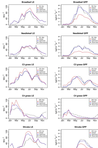
First, each of the sites was optimised individually in order to find site-specific parameter vectors. Typically, this required about 150 function evaluations to find a local optimum. As described in Sect. 2.4, 1-year runs at the different sites were optimised against monthly averaged LE and GPP. The con-stant of proportionalityλis set to 1 for all sites, in order to give equal weighting to both terms in Eq. (5). A site domi-nated by each PFT was picked to represent the general im-provements made. The main seasonal cycles of LE and GPP for the different sites are shown in Fig. 2.
Most broadleaf sites follow the pattern illustrated (Fig. 2, top row). Normally, for broadleaf sites, a standard JULES run
will underestimate GPP. The optimisation does a good job in correcting this, bringing the modelled time series closer to the observations. In contrast, LE does not improve as much.
Similarly for the needleleaf sites (Fig. 2, second row), the JULES model output tends to overestimate LE and underes-timate GPP. The parameter vector found in the optimisation improves the fit of both data streams, most notably GPP. At sites for which a double peak seasonality is apparent, the op-timised model captures this better than the original model.
GPP is also underestimated for the C3 grass sites (Fig. 2, middle row) and, for the majority of the sites, the optimisa-tion does a good job of correcting this. The LE flux tends to have the right magnitude before optimisation, unlike the GPP flux, but adJULES does not manage to improve this output significantly. In the example shown, the JULES model using the default parameter vector already performs very well, so little improvement is needed, but this is not always the case. The new set of parameters is also good at simulating multiple peaks in the LE and GPP fluxes, when they are observed.
There are only two C4 grass sites in the set and JULES does not perform very well on these before or after optimisa-tion (Fig. 2, fourth row). The original stomatal conductance– photosynthesis model within JULES was developed based on fluxes measured over C4 grass as part of the FIFE field ex-periment (Cox et al., 1998). However, there are relatively few FLUXNET sites over C4-dominated landscapes, and only two in the extended data set used here. As a result, the sensi-tivity of stomatal conductance and photosynthesis to environ-mental factors has been less well tested for C4 grasses. The results presented in this paper therefore highlight the need to reassess JULES and other land-surface models for predomi-nantly C4 landscapes.
The shrub sites show no general pattern (Fig. 2, fourth row). Some sites overestimate LE, whilst others underesti-mate it, and similarly for GPP. The level of improvement varies over sites. For some of the sites in this PFT, the mag-nitude of GPP fails to get close to the magmag-nitude of the ob-servations, both before and after optimisation. However, it is hard to pick out a general pattern for this PFT, since there are only five sites in this set.
Overall, the adJULES system works well in finding op-timal parameter vectors, which improve the performance of JULES at individual sites, regardless of PFT. The systematic underestimation of GPP in default JULES improves the most. This larger improvement in the GPP fit reflects the larger set of optimised parameters that are exclusively related to the carbon cycle. Different parameters may need to be incorpo-rated, for example some soil ones, for the LE flux to improve further.
3.2 PFT-specific optimal parameter values
Jan Mar May Jul Sep Nov
0
40
80
120
Broadleaf LE
Wm
−
2
DK−Sor Default Optimised observations
Jan Mar May Jul Sep Nov
0
40
80
120
Needleleaf LE
Wm
−
2
DE−Wet
Default Optimised Observations
Jan Mar May Jul Sep Nov
0
40
80
120
C3 grass LE
Wm
−
2
US−Goo
Default Optimised Observations
Jan Mar May Jul Sep Nov
0
40
80
120
C4 grass LE
Wm
−
2
BW−Ma1
Default Optimised Observations
Jan Mar May Jul Sep Nov
0
40
80
120
Shrubs LE
Wm
−
2
US−Los
Default Optimised Observations
Jan Mar May Jul Sep Nov
0123456
Broadleaf GPP
kg
C
m
−
2yr
−
1
DK−Sor
default optimised observations
Jan Mar May Jul Sep Nov
0123456
Needleleaf GPP
kg
C
m
−
2yr
−
1
DE−Wet
Default Optimised Observations
Jan Mar May Jul Sep Nov
01234
56
C3 grass GPP
kg
C
m
−
2yr
−
1
US−Goo Default Optimised Observations
Jan Mar May Jul Sep Nov
0123456
C4 grass GPP
kg
C
m
−
2yr
−
1
BW−Ma1
Default Optimised Observations
Jan Mar May Jul Sep Nov
0123
456
Shrubs GPP
kg
C
m
−
2yr
−
1
US−Los Default Optimised Observations
2
Figure 2.Time-series plots for illustrative site-specific evaluations showing LE (left) and GPP (right) for each of the different PFTs.
Obser-vations (black) are compared to JULES runs using default parameters (red) and site-specific optimal parameters (blue).
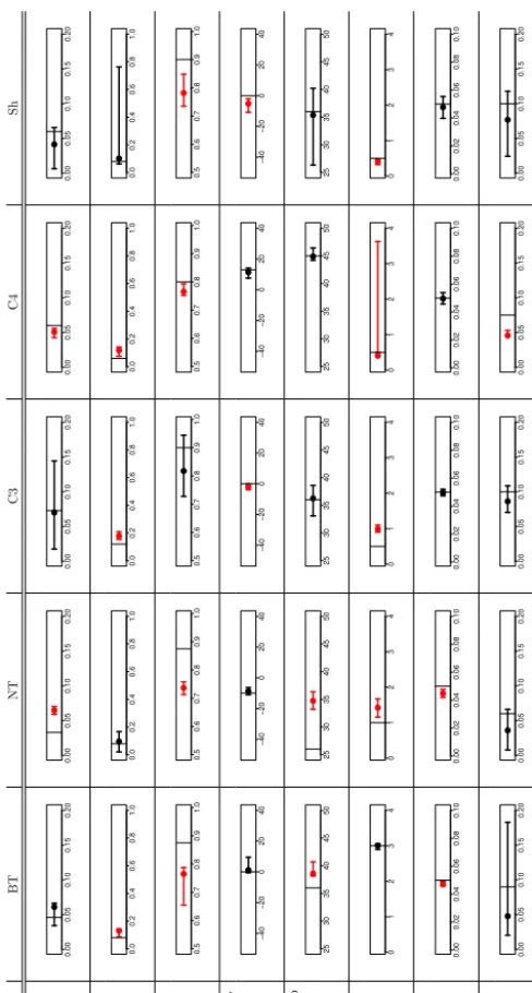
For half of the parameters, the prior parameter value lies outside the posterior uncertainty bounds. The δcδl parameter, which determines the efficiency of rainfall interception by the plant canopy, does not change much from its original value for any of the PFTs. The uncertainty bounds are rela-tively tight and symmetrical. The rest of the parameters show more variation. As described in Sect. 2.5.1, the optimal val-ues need not be in the centre of the uncertainty range, the PDF (probability density function) can be skewed. Most of the PFTs display high uncertainty in at least one of the
pa-rameters optimised; for the optimised broadleaf set for ex-ample,dqc is highly unconstrained. For C4 grasses,dris so unconstrained that the optimal value found lies outside the 80 % confidence interval. C3 grasses show large uncertainty inn0 and, for shrubs, the parameter with the largest uncer-tainty isα.
BT NT C3 C4 Sh nl0 0.00 0.05 0.10 0.15 0.20 0.00 0.05 0.10 0.15 0.20 0.00 0.05 0.10 0.15 0.20 0.00 0.05 0.10 0.15 0.20 0.00 0.05 0.10 0.15 0.20 ↵ 0.0 0.2 0.4 0.6 0.8 1.0 0.0 0.2 0.4 0.6 0.8 1.0 0.0 0.2 0.4 0.6 0.8 1.0 0.0 0.2 0.4 0.6 0.8 1.0 0.0 0.2 0.4 0.6 0.8 1.0 f0 0.5 0.6 0.7 0.8 0.9 1.0 0.5 0.6 0.7 0.8 0.9 1.0 0.5 0.6 0.7 0.8 0.9 1.0 0.5 0.6 0.7 0.8 0.9 1.0 0.5 0.6 0.7 0.8 0.9 1.0 Tlo w − 40 − 20 0 20 40 − 40 − 20 0 20 40 − 40 − 20 0 20 40 − 40 − 20 0 20 40 − 40 − 20 0 20 40 Tupp 25 30 35 40 45 50 25 30 35 40 45 50 25 30 35 40 45 50 25 30 35 40 45 50 25 30 35 40 45 50 rd 01234 01234 01234 01234 01234 c l 0.00 0.02 0.04 0.06 0.08 0.10 0.00 0.02 0.04 0.06 0.08 0.10 0.00 0.02 0.04 0.06 0.08 0.10 0.00 0.02 0.04 0.06 0.08 0.10 0.00 0.02 0.04 0.06 0.08 0.10 dq c 0.00 0.05 0.10 0.15 0.20 0.00 0.05 0.10 0.15 0.20 0.00 0.05 0.10 0.15 0.20 0.00 0.05 0.10 0.15 0.20 0.00 0.05 0.10 0.15 0.20
Figure 3. Summary of PFT-specific optimal JULES parameters
found in this study (Table 1). The error bars show the uncertainty ranges given as an 80 % quantile interval. The range of each box is the prior range of the parameters. Highlighted in red are the error bars for which the prior values (vertical line) are found outside the posterior uncertainty bounds. A numerical version of this figure is given in Table B1.
part of the prior ranges. The cloud of plausible points tends to be restrictive and tight for most parameters.
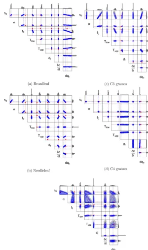
Figure 4 shows clear correlation of some parameters, es-pecially for the tree PFTs. Many of these correlations can be understood in terms of the underlying structure of the JULES model (Sect. 2.1). For example, the positive correlation of n0withf0, and the negative correlation ofn0withdqc, are
consistent with adJULES attempting to fit the stomatal con-ductanceg, which controls the transpiration flux from taller vegetation. The stomatal conductance has the approximate form
g≈1.6A ca
1 (1−f0)+f0dqdqc
!
(10)
if it is assumed thatc∗ciandc∗ca.
The maximum rate of leaf photosynthesis is controlled largely by the leaf nitrogen contentn0, especially in this big-leaf version of JULES (Cox et al., 1999). The best-fit param-eters for tree PFTs also seem to imply that the second term in the denominator dominates over the first. As a result, main-taining a realisticgvalue, and therefore a realistic LE flux, will require thatn0andf0vary proportionally, and that n0 anddqc values are negatively correlated. This is consistent with Fig. 4a and b.
Such correlation of parameters is less obvious for the grass PFTs, because evapotranspiration is controlled less by stom-atal conductance and more by the smaller aerodynamic con-ductances associated with shorter vegetation.
Choice ofλ had less effect on the values of the optimal parameters than on uncertainties and correlations found. The uncertainty ranges become larger with smaller valuesλand correlations less pronounced.
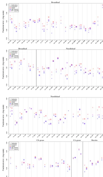
3.3 Assessment of PFT-specific optimal parameters The performance of the PFT-specific parameters is now com-pared to the default JULES values and to the parameters found by optimising independently at each measurement site. For each site, the fractional error in both the calibration year and the evaluation year is displayed Fig. 5.
By definition, the fractional error in calibration years de-creases when moving from default to site-specific optimal parameters in the calibration years. Remarkably, the site-specific optimal parameters also improve the model–data fit in evaluation years for 59/64 (92 %) of sites. Similarly, the PFT-specific optimal parameter vector improves the fit (in both calibration and evaluation years) for 85 % of the sites; 75/79 sites for the calibration years and 55/64 sites for the evaluation years.
Consider first the broadleaf sites (Fig. 5, top two rows). For the majority of sites displayed in the top broadleaf panel, the reduction in fractional error in moving from default to site-specific optimal parameters is substantial and sometimes as much as a factor of 2. In the calibration year, the PFT-specific optimal parameter vector improves 26 of the 27 broadleaf sites shown although one of the sites, IT-Lec, the fit shows no change. The improvement is typically about half as good (on a log scale) as the improvement using the site-specific opti-mal parameters. In other words, the reduction in fractional er-ror moving from default to PFT-specific optimal parameters is sometimes as much as a factor of
√
Figure 4.The correlations between parameters for PFT-specific parameter optimisations. Each subfigure shows a 2-D correlation map, within which each box is a 2-D marginal plot. Bar graphs show 1-D marginal distributions for individual parameters. The dimensions of the boxes represent the prior range of each parameter. Red points/dashed lines represent initial parameter values. Blue points/dashed lines represent optimised parameter values. Blue contours illustrate the posterior distribution.
sites, only UK-PL3 gets notably worse. Investigation shows that this site behaves differently from the rest of the sites in the set, both in the magnitude of the fluxes and seasonality. This UK site is in the Pang–Lambourn catchment, which has chalk soil with macropores that permit significant lateral sub-surface flows of soil moisture. These horizontal flows cannot
be captured in a model like JULES, which is essentially 1-D in the vertical below the soil surface.
Taylor diagram for LE improvements at BT sites
Normalised standard deviation
N o rm a lis e d st a n d a rd de v ia ti o n
0.0 0.5 1.0 1.5 2.0
0.0 0.5 1.0 1.5 2.0 0.5 1 1.5 2 ● 0.1 0.2 0.3 0.4 0.5 0.6 0.7 0.8 0.9 0.95 0.99 Correlation ● ● ● ● ● ● ● ● ● ● ● ● ● ● ● ●● ● ● ● ● ● ● ● ● ● ● ● ● ● ● ●● ● ●● ● ●● ● ●● ● ● ● ● ● ● ● ● ● ● ● ● ● ● ● ● ● ● ● ● ●●● ● ● ● ● ● ● ● ● ●● ● ●● ● ●● ● ●● ● ● ● ● ● ● ● ● ● ●● ● ●● ●●● ● ● ● ● ● ● ● ● ● ● ● ● ● ● ● ● ● ● ● ● ● ● ● ● ● ●● ● ●● ● ● ● ● ● ● ● ● ● ●● ● ● ●● ● ●● ● ● ● ●●● ●
Taylor diagram for GPP improvements at NT sites
Normalised standard deviation
N o rm a lis e d st a n d a rd de v ia ti o n
0.0 0.5 1.0 1.5 2.0
0.0 0.5 1.0 1.5 2.0 0.5 1 1.5 2 ● 0.1 0.2 0.3 0.4 0.5 0.6 0.7 0.8 0.9 0.95 0.99 Correlation ● ● ● ● ● ● ● ● ● ● ● ● ●●● ●●● ● ● ● ● ● ● ● ● ● ● ● ● ● ● ● ● ● ● ● ● ● ● ● ● ● ● ● ● ● ● ● ● ● ● ● ● ● ● ● ● ● ● ● ● ● ● ● ● ● ●● ● ●● ● ● ● ● ● ● ● ● ● ● ● ● ● ● ● ● ● ● ● ● ● ● ● ● ● ● ● ● ● ● ● ● ● ● ● ● ●●● ●●● ● ●● ● ●● ● ● ● ● ● ● ● ● ● ● ● ● ● ● ● ● ● ● ● ● ● ● ● ● ● ● ● ● ● ● ● ●● ● ●● ● ●● ● ●● ● ● ● ● ● ● ● ● ● ● ● ● ● ● ● ● ● ● ● ● ● ● ● ● ● ● ● ● ● ● ● ● ● ● ● ●
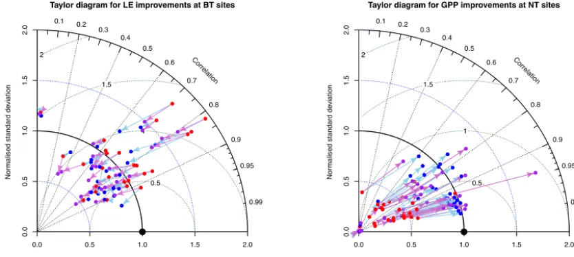
Figure 1: Improvements in fit represented by ‘Taylor diagrams’. Observed timeseries (black dot) can be com-pared with modelled timeseries for default parameters (red dots), site–specific optimal parameters (blue dots) and PFT–generic optimal parameters (purple dots). Radial distance from the origin (dotted lines) represents normalised standard deviationpvar(mt)/var(ot), and so a modelled time series with the correct variance lies
on the thick black line. Angular position represents the correlation between modelled and observed timeseries. The distance from the black dot (dotted green lines) represents the normalised standard deviation in the errors
p
var(ot mt)/var(ot).
1
Analysis of improvement in fit
The fractional error is a good tool for cross-site comparison but it does not give much information about the way in which the optimised parameter vectors improve the fit at each site. Taylor diagrams ([?]) provide more insight into how the fit has been improved by considering the relationship between observed variancevar(ot),
modelled variancevar(mt), error variancevar(ot mt) and model–observation correlationcor(ot,mt).
The Taylor diagrams in Fig. 1 illustrate the improvement in performance of the optimised model for both the site–specific and PFT–generic parameters during calibration years (plots for validation years are very similar). For latent heat at broadleaf sites (left), the improvement is most noticeable in cases where the seasonal cycle was overestimated. The correlation between the modelled time-series and observation time-series does not improve much but for the majority of the sites this starts o↵ relatively high (over 0.6). Other PFTs show less drastic improvements for latent heat.
For GPP at needeleaf sites (right), the seasonal cycle is typically underestimated and improves notieceably for both the single–site parameter vectors and the PFT–generic parameter vectors. The correlation between model and observed time-series does not change greatly. The Taylor diagram for GPP at broadleaf sites is very similar. For grasses and shrubs, the change is less drastic, though some of the sites have a more notable increase in correlation.
Since Taylor diagrams are based on a decomposition of the variance of the errors they are insensitive to any systematic o↵set in the model. It therefore makes sense to consider in addition the normalised bias|µm µo|/ o.
Calculating this statistic separately shows a reduction in bias for nearly all sites. Taken together, these measures show that the observed improvements in model fit are due mainly to adjustment of the magnitude of the annual cycle and reduction in bias.
Figure 6.Improvements in fit represented by “Taylor diagrams”. Observed time series (black dot) can be compared with modelled time
series for default parameters (red dots), site-specific optimal parameters (blue dots) and PFT-generic optimal parameters (purple dots). Radial distance from the origin (dotted lines) represents normalised standard deviation√var(mt)/var(ot), and so a modelled time series with the correct variance lies on the thick black line. Angular position represents the correlation between modelled and observed time series. The distance from the black dot (dotted green lines) represents the normalised standard deviation in the errors√var(ot−mt)/var(ot).
For AU-Tum, the PFT-specific parameter vector outperforms the site-specific vector. This illustrates that the PFT-specific vector can be robust, whereas the locally optimised vectors might over-tune to the specific behaviour of the calibration year.
Results are similar for the needleleaf sites, the majority of the sites show noticeable improvements in both the calibra-tion and evaluacalibra-tion years when using site-specific optimal parameter vectors. For over a third of the sites in this PFT, the improvement when using the PFT-specific parameter vec-tor is similar to that obtained with the site-specific parame-ter vector. This illustrates that these sites fit well together as a single PFT. For these sites, the PFT-specific vector some-times outperforms the site-specific vector on the evaluation years. Some sites in the needleleaf PFT remain unchanged regardless of the parameter vector used. Anomalous sites that should be noted are Qcu, SF3 and US-Blo. The CA-Qcu site is the only one in this PFT that does not improve when using the PFT-specific vector, for either the calibration or evaluation years. This site has a lower annual cycle of GPP than the rest in this set. The CA-SF3 site improves when us-ing the site-specific parameter vector in the evaluation year, but not using the PFT-specific vector. The US-Blo site im-proves in the calibration year, but when confronted with the evaluation year, both the site-specific vector and PFT-specific vector worsen the fit. This evaluation year has unusually high LE, which might be causing this discrepancy.
For some sites, (e.g. US-Blo and BW-Ma1), the PFT-specific optimum outperforms the site-PFT-specific optimum in the calibration year. This phenomenon was also noted by Kuppel et al. (2014), who suggest that the added constraints
placed on the parameters by increasing the number of sites causes the cost function to become “smoother”. This may render the optimisation scheme less likely to become trapped in local minima.
The last panel of Fig. 5 shows the C3 grass sites, the C4 grass sites and the shrubs sites. For the C3 grass sites, the ma-jority of the evaluation years have a better fit with the PFT-specific parameter vector than with site-PFT-specific parameter vector. This suggests that the seasonal cycle differs over the different years at these sites. For the C4 grass sites, which started with relatively high errors, the new parameter vectors improve the sites slightly for the calibration year but hardly at all for the evaluation year. This set of two sites is too small to draw any proper conclusion about the C4 grass parame-ters. There is a clear need for more data from C4 grass sites. Finally, the shrubs can be seen to improve for all the sites. For the shrub sites, both the site-specific and the PFT-specific provide a better fit of the model to the observations of the calibration year. The improvement is minor for these sites, except for CA-Mer, which halves its fractional error. When confronted with observations from the evaluation years, the model also improves the fit of these sites for both site-specific and PFT-specific parameters (with the exception of US-Los, where the site-specific optimal vector increases error but the PFT-specific vector reduces it). This is another example of the PFT-specific parameter vector being more robust. 3.4 Analysis of improvement in fit
Taylor diagrams (Taylor, 2001) provide more insight into how the fit has been improved by considering the relation-ship between observed variance var(ot), modelled variance var(mt), error variance var(ot−mt)and model–observation correlation cor(ot,mt).
The Taylor diagrams in Fig. 6 illustrate the improvement in performance of the optimised model for both the site-specific and PFT-generic parameters during calibration years (plots for evaluation years are very similar).
For latent heat at broadleaf sites (left), the improvement is most noticeable in cases where the seasonal cycle was over-estimated. The correlation between the modelled time series and observation time series does not improve much but for the majority of the sites this starts off relatively high (over 0.6). Other PFTs show less drastic improvements for latent heat.
For GPP at needleleaf sites (right), the seasonal cycle is typically underestimated and improves noticeably for both the single-site parameter vectors and the PFT-generic param-eter vectors. The correlation between model and observed time series does not change greatly. The Taylor diagram for GPP at broadleaf sites is very similar. For grasses and shrubs, the change is less drastic, though some of the sites have a more notable increase in correlation.
Since Taylor diagrams are based on a decomposition of the variance of the errors they are insensitive to any systematic offset in the model. It therefore makes sense to consider in addition the normalised bias|µm−µo|/σo. Calculating this statistic separately shows a reduction in bias for nearly all sites. Taken together, these measures show that the observed improvements in model fit are due mainly to adjustment of the magnitude of the annual cycle and a reduction in bias.
4 Conclusions
This study introduces the adJULES system, which has been developed to tune the internal parameters of the JULES land-surface model. adJULES enables objective calibration of JULES against observational data, providing best-fit internal parameters and associated uncertainty ranges.
For individual FLUXNET sites, adJULES has the abil-ity to find local (site-specific) optimal parameter vectors that significantly improve the performance of the JULES model compared to runs generated using the default parameters. The data streams used in the calibration, LE and GPP, are both modelled more accurately with the optimal parameter vectors, with the GPP flux improving the most. The greater improvement in the GPP flux is due to the fact that the pa-rameters considered in this study are mainly related to pho-tosynthesis. For the LE flux to improve more significantly, more water and energy-related parameters would need to be considered in the optimisation.
When optimised locally to find site-specific parameters, all of the sites in this study improve the model–data fit for
the calibration year. In addition, when confronted with in-dependent data from a evaluation year, the locally optimised parameter vectors decreased the error in model–data fit for 92 % of the sites. This evaluation of the site-specific parame-ter vectors is promising, and suggests that the adJULES sys-tem is robust. It also gives confidence that the parameter vec-tors found can be generalised over different locations.
This study is motivated partly by the desire to improve the performance of JULES within the Hadley Centre’s Earth sys-tem models, which means needing to find best-fit parameters for a relatively small number of PFTs. The adJULES system has the ability to calibrate multiple locations simultaneously in order to find best-fit parameters. This multi-site optimisa-tion is a relatively new feature in terrestrial data assimilaoptimisa-tion. By classifying the FLUXNET sites into groups dominated by each JULES PFT (BT, NT, C3G, C4G, Sh), adJULES was used to find the optimal PFT-specific parameters.
Although the PFT-specific optimal parameters do not al-ways fit the data as well as site-specific optimal parame-ters, they still offer significant improvements over the default JULES parameters. For over 85 % of the sites, PFT-specific optimal parameters perform better than default parameters when confronted with independent evaluation data. For 50 % of the sites, the PFT-specific optimal parameters perform at least as well as site-specific optimal parameters. This implies that the multi-site methodology is less susceptible to over-tuning, both in terms of variability across sites (e.g. different overground biomass and tree ranges), and in terms of vari-ability through time (e.g. unusually high rainfall in the cali-bration year).
The PFT-specific parameters found in this study represent a significant improvement on the default ones. The fact that such parameters could be found implies robust parameterisa-tions independent of geography. This supports the idea that it is possible to represent global vegetation with a relatively small number of PFTs.
A successful and robust multi-site optimisation assumes that sites can be grouped and parameter values can apply to several sites at once. Whilst the PFT-specific parameters show great improvement, agreeing with the use of five PFTs in JULES, it would be possible to rethink the PFT defini-tions and group sites differently. This could be done either by looking more closely at the site specifics detailed in the FLUXNET database, or by considering single-site optimisa-tions and performing a cluster analysis in parameter space to identify PFTs empirically.
It is however clear that there are some limitations to the success of the optimisation results. Some sites still show sig-nificant differences between model output and observations. This suggests that an improvement to model physics may be necessary in order to produce better model output. This is because adJULES produces the (locally) best possible fit to observations, given the existing model physics and the pre-scribed driving data. If the fit is still inadequate, this may be due to the model and data themselves, rather than parameter values. adJULES can therefore be used in the identification of model structural errors. Another reason for inadequate fit may be due to the method used. A limitation of gradient de-scent methods, such as the optimisation scheme used in this study, is that the local minimum found depends on the ini-tial parameter vector. However, as discussed in Sect. 3.3, the fact that the cost function becomes smoother with additional sites may help with becoming trapped in local minima (Kup-pel et al., 2014). Alternative methods, including ensemble methods, could avoid this issue, but are more computation-ally costly. For some PFTs (notably C4G and shrubs) there are insufficient FLUXNET sites to determine optimal param-eters satisfactorily. Additional data and sites for these PFTs are therefore urgently required.
5 Code availability
Appendix A
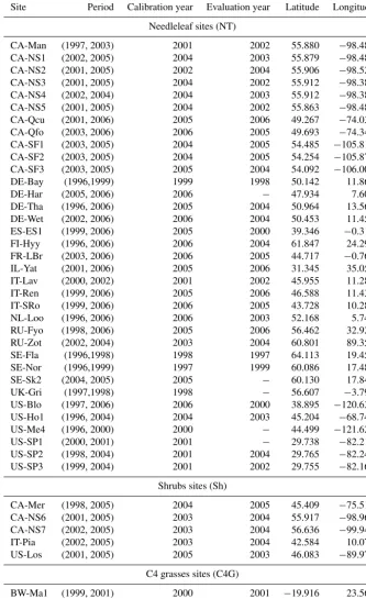
Table A1.FLUXNET sites used in this study, labelled by a country code (first two letters) and site name (last three letters). The period
corresponds to the available years of data for each of the sites.
Site Period Calibration year Evaluation year Latitude Longitude
Broadleaf sites (BT)
DE-Hai (2000, 2006) 2005 2004 51.079 10.452
DK-Sor (1996, 2006) 2006 2004 55.487 11.646
FR-Fon (2005, 2006) 2006 − 48.476 2.780
FR-Hes (1997, 2006) 2003 1998 48.674 7.065
IT-Col (1996, 2006) 2005 2001 41.849 13.588
IT-LMa (2003, 2006) 2006 2004 45.581 7.155
IT-Non (2001, 2006) 2002 2003 44.690 11.089
IT-PT1 (2002, 2004) 2003 2004 45.201 9.061
IT-Ro1 (2000, 2006) 2006 2005 42.408 11.930
IT-Ro2 (2002, 2006) 2004 2006 42.390 11.921
UK-Ham (2004, 2005) 2005 − 51.121 −0.861
UK-PL3 (2005, 2006) 2006 − 51.450 −1.267
US-Bar (2004, 2005) 2005 − 44.065 −71.288
US-Ha1 (1991, 2006) 1996 1998 42.538 −72.171 US-MMS (1999, 2005) 2002 2003 39.323 −86.413 US-MOz (2004, 2006) 2006 2005 38.744 −92.200 US-UMB (1999, 2003) 2003 2002 45.560 −84.714 US-WCr (1999, 2006) 2005 2000 45.806 −90.080 AU-Tum (2001, 2006) 2003 2005 −35.656 148.152
AU-Wac (2005, 2007) 2006 − −37.429 145.187
BR-Sa1 (2002, 2004) 2003 2004 −2.857 −54.959 BR-Sa3 (2000, 2003) 2002 2003 −3.018 −54.971
FR-Pue (2000, 2006) 2006 2005 43.741 3.596
ID-Pag (2002, 2003) 2003 − 2.345 114.036
IT-Cpz (1997, 2006) 2004 2006 41.705 12.376
IT-Lec (2005, 2006) 2006 − 43.305 11.271
PT-Esp (2002, 2004) 2004 2003 38.639 −8.602
PT-Mi1 (2003, 2005) 2005 − 38.541 −8.000
C3 grasses sites (C3G)
DE-Gri (2005, 2006) 2006 − 50.950 13.512
DK-Lva (2005, 2006) 2006 − 55.683 12.083
ES-LMa (2004, 2006) 2006 2005 39.941 −5.773
HU-Bug (2002, 2006) 2006 2005 46.691 19.601
HU-Mat (2004, 2006) 2006 2005 47.847 19.726
IT-Amp (2002, 2006) 2006 2005 41.904 13.605
PL-wet (2004, 2005) 2005 − 52.762 16.309
PT-Mi2 (2004, 2006) 2006 2005 38.477 −8.025
Table A1.Continued.
Site Period Calibration year Evaluation year Latitude Longitude
Needleleaf sites (NT)
CA-Man (1997, 2003) 2001 2002 55.880 −98.481 CA-NS1 (2002, 2005) 2004 2003 55.879 −98.484 CA-NS2 (2001, 2005) 2002 2004 55.906 −98.525 CA-NS3 (2001, 2005) 2004 2002 55.912 −98.382 CA-NS4 (2002, 2004) 2004 2003 55.912 −98.382 CA-NS5 (2001, 2005) 2004 2002 55.863 −98.485 CA-Qcu (2001, 2006) 2005 2006 49.267 −74.037 CA-Qfo (2003, 2006) 2006 2005 49.693 −74.342 CA-SF1 (2003, 2005) 2004 2005 54.485 −105.818 CA-SF2 (2003, 2005) 2004 2005 54.254 −105.878 CA-SF3 (2003, 2005) 2005 2004 54.092 −106.005
DE-Bay (1996,1999) 1999 1998 50.142 11.867
DE-Har (2005, 2006) 2006 − 47.934 7.601
DE-Tha (1996, 2006) 2005 2004 50.964 13.567
DE-Wet (2002, 2006) 2006 2004 50.453 11.457
ES-ES1 (1999, 2006) 2005 2000 39.346 −0.319
FI-Hyy (1996, 2006) 2006 2004 61.847 24.295
FR-LBr (2003, 2006) 2006 2005 44.717 −0.769
IL-Yat (2001, 2006) 2005 2006 31.345 35.051
IT-Lav (2000, 2002) 2001 2002 45.955 11.281
IT-Ren (1999, 2006) 2005 2006 46.588 11.435
IT-SRo (1999, 2006) 2006 2005 43.728 10.284
NL-Loo (1996, 2006) 2006 2003 52.168 5.744
RU-Fyo (1998, 2006) 2005 2006 56.462 32.924
RU-Zot (2002, 2004) 2003 2004 60.801 89.351
SE-Fla (1996,1998) 1998 1997 64.113 19.457
SE-Nor (1996,1999) 1997 1999 60.086 17.480
SE-Sk2 (2004, 2005) 2005 − 60.130 17.840
UK-Gri (1997,1998) 1998 − 56.607 −3.798
US-Blo (1997, 2006) 2006 2000 38.895 −120.633 US-Ho1 (1996, 2004) 2004 2003 45.204 −68.740
US-Me4 (1996, 2000) 2000 − 44.499 −121.622
US-SP1 (2000, 2001) 2001 − 29.738 −82.219
US-SP2 (1998, 2004) 2001 2004 29.765 −82.245 US-SP3 (1999, 2004) 2001 2002 29.755 −82.163
Shrubs sites (Sh)
CA-Mer (1998, 2005) 2004 2005 45.409 −75.519 CA-NS6 (2001, 2005) 2003 2004 55.917 −98.964 CA-NS7 (2002, 2005) 2003 2004 56.636 −99.948
IT-Pia (2002, 2005) 2003 2004 42.584 10.078
US-Los (2001, 2005) 2005 2003 46.083 −89.979
C4 grasses sites (C4G)
Appendix B
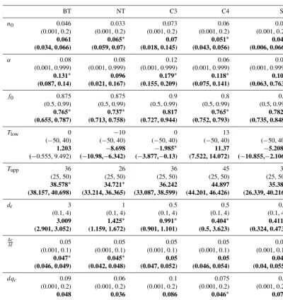
Table B1.PFT-specific JULES parameters optimised in this study (Table 1). The prior values and ranges for each PFT are given. Below in
bold are the optimised values and posterior uncertainty ranges given as an 80 % confidence interval (in parentheses). Optimised values for which the prior values lie outside the posterior range are highlighted by (*). A graphical version of this table is shown in Fig. 3.
BT NT C3 C4 Sh
n0 0.046 0.033 0.073 0.06 0.06
(0.001, 0.2) (0.001, 0.2) (0.001, 0.2) (0.001, 0.2) (0.001, 0.2)
0.061 0.065∗ 0.07 0.051∗ 0.041
(0.034, 0.066) (0.059, 0.07) (0.018, 0.145) (0.043, 0.056) (0.006, 0.066)
α 0.08 0.08 0.12 0.06 0.08
(0.001, 0.999) (0.001, 0.999) (0.001, 0.999) (0.001, 0.999) (0.001, 0.999)
0.131∗ 0.096 0.179∗ 0.118∗ 0.102
(0.087, 0.14) (0.021, 0.167) (0.155, 0.209) (0.075, 0.141) (0.063, 0.763)
f0 0.875 0.875 0.9 0.8 0.9
(0.5, 0.99) (0.5, 0.99) (0.5, 0.99) (0.5, 0.99) (0.5, 0.99)
0.765∗ 0.737∗ 0.817 0.765∗ 0.782∗
(0.655, 0.787) (0.713, 0.758) (0.727, 0.944) (0.752, 0.793) (0.735, 0.848)
Tlow 0 −10 0 13 0
(−50, 40) (−50, 40) (−50, 40) (−50, 40) (−50, 40)
1.203 −8.698 −1.985∗ 11.37 −5.208∗
(−0.555, 9.492) (−10.98,−6.342) (−3.877,−0.13) (7.522, 14.072) (−10.855,−2.106)
Tupp 36 26 36 45 36
(25, 50) (25, 50) (25, 50) (25, 50) (25, 50)
38.578∗ 34.721∗ 36.242 44.897 35.385
(38.157, 40.698) (33.214, 36.365) (33.087, 38.599) (44.201, 46.426) (26.339, 40.216)
dr 3 1 0.5 0.5 0.5
(0.1, 4) (0.1, 4) (0.1, 4) (0.1, 4) (0.1, 4)
3.009 1.425∗ 0.991∗ 0.404∗ 0.411∗
(2.901, 3.052) (1.159, 1.672) (0.901, 1.101) (0.5, 3.623) (0.324, 0.473)
δc
δl 0.05 0.05 0.05 0.05 0.05
(0.001, 0.1) (0.001, 0.1) (0.001, 0.1) (0.001, 0.1) (0.001, 0.1)
0.047∗ 0.045∗ 0.05 0.05 0.048
(0.046, 0.049) (0.042, 0.048) (0.047, 0.052) (0.046, 0.054) (0.04, 0.055)
dqc 0.09 0.06 0.1 0.075 0.1
(0.001, 0.2) (0.001, 0.2) (0.001, 0.2) (0.001, 0.2) (0.001, 0.2)
0.048 0.036 0.086 0.046∗ 0.077
Acknowledgements. This work was supported by the UK Natural Environment Research Council (NERC) through the National Cen-tre for Earth Observation (NCEO).
This study used eddy-covariance data acquired by the FLUXNET community and in particular by the following networks: Amer-iFlux (US Department of Energy, Biological and Environmental Research, Terrestrial Carbon Program (DE-FG02-04ER63917 and DE-FG02-04ER63911)), AfriFlux, AsiaFlux, CarboAfrica, Car-boEuropeIP, CarboItaly, CarboMont, ChinaFlux, Fluxnet-Canada (supported by CFCAS, NSERC, BIOCAP, Environment Canada, and NRCan), GreenGrass, KoFlux, LBA, NECC, OzFlux, TCOS-Siberia, USCCC. Support for eddy-covariance data harmonisation was provided by CarboEuropeIP, FAO-GTOS-TCO, iLEAPS, Max Planck Institute for Biogeochemistry, National Science Foundation, University of Tuscia, Université Laval and Environment Canada and US Department of Energy and the database development and technical support from Berkeley Water Center, Lawrence Berkeley National Laboratory, Microsoft Research eScience, Oak Ridge Na-tional Laboratory, University of California – Berkeley, University of Virginia.
The authors are grateful to T. Kaminski and R. Giering from FastOpt for their contribution to the development of the adjoint model, and to M. Groenendijk, A. Harper, and the UK Met Office for processing and sharing their data.
The authors are particularly grateful to two anonymous referees for their thoughtful and constructive reviews, which greatly improved this manuscript.
Edited by: J. Kala
Reviewed by: H. Gupta and three anonymous referees
References
Ajami, N. K., Duan, Q., and Sorooshian, S.: An integrated hy-drologic Bayesian multimodel combination framework: Con-fronting input, parameter, and model structural uncertainty in hydrologic prediction, Water Resour. Res., 43, w01403, doi:10.1029/2005WR004745, 2007.
Arora, V. and Boer, G.: A parameterization of leaf phenology for the terrestrial ecosystem component of climate models, Glob. Change Biol., 11, 39–59, 2005.
Baldocchi, D., Falge, E., Gu, L., Olson, R., Hollinger, D., Running, S., Anthoni, P., Bernhofer, C., Davis, K., Evans, R., Fuentes, J., Goldstein, A., Katul, G., Law, B., Lee, X., Malhi, Y., Meyers, T., Munger, W., Oechel, W., Paw U, K. T., Pilegaard, K., Schmid, H. P., Valentini, R., Verma, S., Vesala, T., Wilson, K., and Wofsy, S.: FLUXNET: a new tool to study the temporal and spatial variabil-ity of ecosystem-scale carbon dioxide, water vapor, and energy flux densities, B. Am. Meteorol. Soc., 82, 2415–2434, 2001. Bartholomew-Biggs, M., Brown, S., Christianson, B., and Dixon,
L.: Automatic differentiation of algorithms, J. Comput. Appl. Math., 124, 171–190, doi:10.1016/S0377-0427(00)00422-2, 2000.
Best, M. J., Pryor, M., Clark, D. B., Rooney, G. G., Essery, R. L. H., Ménard, C. B., Edwards, J. M., Hendry, M. A., Porson, A., Gedney, N., Mercado, L. M., Sitch, S., Blyth, E., Boucher, O., Cox, P. M., Grimmond, C. S. B., and Harding, R. J.: The Joint UK Land Environment Simulator (JULES), model description –
Part 1: Energy and water fluxes, Geosci. Model Dev., 4, 677–699, doi:10.5194/gmd-4-677-2011, 2011.
Blyth, E., Lloyd, A., Gash, J., Pryor, M., Weedon, G., and Shut-tleworth, J.: Evaluating the JULES Land Surface Model Energy Fluxes Using FLUXNET Data, J. Hydrometeorol., 11, 509–519, 2010.
Booth, B. B. B., Dunstone, N. J., Halloran, P. R., Andrews, T., and Bellouin, N.: Aerosols implicated as a prime driver of twentieth-century North Atlantic climate variability, Nature, 484, 228–232, 2012.
Bouttier, F. and Courtier, P.: Data assimilation concepts and meth-ods, Training, 1–59, Meteorological training course lecture se-ries, ECMWF, 1999.
Braswell, B. H., Sacks, W. J., Linder, E., and Schimel, D. S.: Estimating diurnal to annual ecosystem parameters by synthe-sis of a carbon flux model with eddy covariance net ecosys-tem exchange observations, Glob. Change Biol., 11, 335–355, doi:10.1111/j.1365-2486.2005.00897.x, 2005.
Brovkin, V., Boysen, L., Raddatz, T., Gayler, V., Loew, A., and Claussen, M.: Evaluation of vegetation cover and land-surface albedo in MPI-ESM CMIP5 simulations, J. Adv. Model. Earth Syst., 5, 48–57, doi:10.1029/2012MS000169, 2013.
Byrd, R., Lu, P., Nocedal, J., and Zhu, C.: A limited memory al-gorithm for bound constrained optimization, SIAM Journal on Scientific Computing, 16, 1190–1208, 1995.
Clark, D. B., Mercado, L. M., Sitch, S., Jones, C. D., Gedney, N., Best, M. J., Pryor, M., Rooney, G. G., Essery, R. L. H., Blyth, E., Boucher, O., Harding, R. J., Huntingford, C., and Cox, P. M.: The Joint UK Land Environment Simulator (JULES), model descrip-tion – Part 2: Carbon fluxes and vegetadescrip-tion dynamics, Geosci. Model Dev., 4, 701–722, doi:10.5194/gmd-4-701-2011, 2011. Collatz, G., Ball, J., Grivet, C., and Berry, J.: Physiological and
en-vironmental regulation of stomatal conductance, photosynthesis and transpiration: a model that includes a laminar boundary layer, Agr. Forest Meteorol., 54, 107–136, 1991.
Collatz, G. J., Ribas-Carbo, M., and Berry, J.: Coupled photosynthesis-stomatal conductance model for leaves of C4 plants, Funct. Plant Biol., 19, 519–538, 1992.
Cox, P., Huntingford, C., and Harding, R.: A canopy conductance and photosynthesis model for use in a GCM land surface scheme, J. Hydrol., 212, 79–94, 1998.
Cox, P., Betts, R., Jones, C., Spall, S., and Totterdell, I.: Accelera-tion of global warming due to carbon-cycle feedbacks in a cou-pled climate model, Nature, 408, 184–187, 2000.
Cox, P. M., Betts, R. A., Bunton, C. B., Essery, R. L. H., Rown-tree, P. R., and Smith, J.: The impact of new land surface physics on the GCM simulation of climate and climate sensitivity, Clim. Dynam., 15, 183–203, 1999.
Friedlingstein, P., Bopp, L., Ciais, P., Dufresne, J.-L., Fairhead, L., LeTreut, H., Monfray, P., and Orr, J.: Positive feedback between future climate change and the carbon cycle, Geophys. Res. Lett., 28, 1543–1546, doi:10.1029/2000GL012015, 2001.