Real‑time inverse kinematics for the
upper limb: a model‑based algorithm using
segment orientations
Bence J. Borbély
*and Péter Szolgay
Background
Quantitative movement analysis is a key concept in understanding processes of the human movement system. Evolved, high precision measurement devices have advanced
Abstract
Background: Model based analysis of human upper limb movements has key impor-tance in understanding the motor control processes of our nervous system. Various simulation software packages have been developed over the years to perform model based analysis. These packages provide computationally intensive—and therefore off-line—solutions to calculate the anatomical joint angles from motion captured raw measurement data (also referred as inverse kinematics). In addition, recent develop-ments in inertial motion sensing technology show that it may replace large, immobile and expensive optical systems with small, mobile and cheaper solutions in cases when a laboratory-free measurement setup is needed. The objective of the presented work is to extend the workflow of measurement and analysis of human arm movements with an algorithm that allows accurate and real-time estimation of anatomical joint angles for a widely used OpenSim upper limb kinematic model when inertial sensors are used for movement recording.
Methods: The internal structure of the selected upper limb model is analyzed and used as the underlying platform for the development of the proposed algorithm. Based on this structure, a prototype marker set is constructed that facilitates the reconstruc-tion of model-based joint angles using orientareconstruc-tion data directly available from inertial measurement systems. The mathematical formulation of the reconstruction algorithm is presented along with the validation of the algorithm on various platforms, including embedded environments.
Results: Execution performance tables of the proposed algorithm show significant improvement on all tested platforms. Compared to OpenSim’s Inverse Kinematics tool 50–15,000x speedup is achieved while maintaining numerical accuracy.
Conclusions: The proposed algorithm is capable of real-time reconstruction of standardized anatomical joint angles even in embedded environments, establishing a new way for complex applications to take advantage of accurate and fast model-based inverse kinematics calculations.
Keywords: Inverse kinematics (IK), Inertial measurement unit (IMU), Real-time, Upper limb, OpenSim, Embedded systems, Wearable
Open Access
© The Author(s) 2017. This article is distributed under the terms of the Creative Commons Attribution 4.0 International License (http://creativecommons.org/licenses/by/4.0/), which permits unrestricted use, distribution, and reproduction in any medium, provided you give appropriate credit to the original author(s) and the source, provide a link to the Creative Commons license, and indicate if changes were made. The Creative Commons Public Domain Dedication waiver (http://creativecommons.org/publicdo-main/zero/1.0/) applies to the data made available in this article, unless otherwise stated.
RESEARCH
research activity in movement rehabilitation [1–4], performance analysis of athletes [5] and general understanding of the motor system [6–9] during the last decades by mak-ing movement pattern comparison possible. This advancement was further accelerated by model-based analysis approaches that enabled explicit characterization of the studied movement patterns [10–15].
The most widely used measurement systems apply line-of-sight (LoS) methods (optical or ultrasound-based) that require a fixed marker-sensor structure. In these cases passive (optical) or active (ultrasound) markers are placed on anatomically relevant locations of the studied subject. Having the markers in place, measurements have to be performed in a specialized laboratory environment where locations and orientations of the sensor elements (i.e. cameras or microphones) are known and invariant (at least across trials). This means that even the spatial positions of the markers can be determined with good accuracy—especially with optical systems—the possible range of motion will always be constrained by the actual measurement volume covered by the sensors of the system. Although this property is not an issue for many movement analysis scenarios, there are cases when a measurement method allowing unconstrained free space movement would be more beneficial (e.g. various outdoor activities or ergonomic assessment of work environments, to name a few).
Advancements in the field of inertial sensor technology have given rise to new devel-opment directions in laboratory-free movement analysis methods. The main difference between LoS and inertial systems is the recorded modality: while LoS methods deter-mine the spatial locations of markers based on planar position (optical) or timing (ultra-sound) information, inertial sensors give their orientation in space by measuring physical quantities acting on them directly. These quantities are linear acceleration and angular velocity in most cases while they are supplemented with magnetic field measurements in more complete setups. To obtain orientation from raw inertial measurements, various sensor fusion algorithms have been developed utilizing Kalman-filters [16, 17], gradient descent methods [18], complementary filters [19, 20] and other techniques [21], most of them being capable for real-time operation in embedded systems. In addition, recent evolution of chip-scale inertial sensors based on MEMS technology further widened the possibilities of wearable measurement device development by making the core sensing elements available for better integration. While there is no gold standard among fusion algorithms and sensor chips as compromises have to be made in aspects of accuracy, system complexity and computational demand of the fusion algorithm, it can be stated that inertial sensor technology is taking a more and more growing part in human move-ment measuremove-ments (a good example for this progress is Xsens’ product portfolio).
model includes 15 degrees of freedom and 50 muscle compartments and in addition to movement kinematics it enables the evaluation of muscle-tendon lengths, moment arms, muscle forces and joint moments in an anatomically reasonable setup (also con-forming to the ISB recommendation [27] as those presented in [23] and [24]). Our moti-vation of choosing this approach instead of using direct joint kinematics estimates from inertial sensor data lies in the strong belief that the utilization of this upper limb model leads to better understanding of the additional inherent properties of arm movements (e.g. muscle activation patterns) compared to a pure kinematic investigation.
By using the model from [26], two main differences from the direct approach should be considered: (1) because the model was developed mainly for optical motion capture technology, joint angle reconstruction is less coupled with raw measurement data in the sense that it is performed as an inverse task based on locations of arbitrarily placed vir-tual markers (instead of relying on sensor orientations directly) and (2) as a consequence of the inverse kinematics approach, the model raises more computational demand for joint angle reconstruction. While the first point contributes to a possibly wider adoption of the model (i.e. measurement data of any reasonable source—being it optical, ultra-sound based, inertial, etc.—only needs to be expressed in terms of virtual marker loca-tions), the second can be considered as a drawback in certain situations when real-time joint angle reconstruction would be beneficial.
To analyze model-defined parameters of recorded movements, various software pack-ages have been developed for biomechanical analysis over the past decades. Some of them are tightly integrated into their corresponding measurement system’s ecosystem with only kinematic reconstruction capabilities [28–30] while others are independent of a particular hardware setup (SIMM [31] and OpenSim [32]), even including analysis options for muscle activations and movement dynamics if the corresponding models are available. While these tools may address the joint angle reconstruction problem involv-ing inverse kinematics in different ways resultinvolv-ing in varyinvolv-ing performance, OpenSim [32] was chosen as the reference model-based analysis software for the purposes of the cur-rent study, because (as to the best of the authors’ knowledge) it is the only free and open source (thus widely accessible) option in the biomechanical modeling field.
Because the upper limb model used in this study was originally developed for the SIMM software, an other reason for using OpenSim was it’s ability to import and han-dle SIMM models natively, so combined with the model it provides a complete pack-age for open source arm movement analysis. For kinematic evaluation, OpenSim uses the “standard” offline measurement-scaling-inverse kinematics pipeline where the actual biomechanical model (single limb to full body) is fitted to measurement data. During this process, positions of virtual markers placed on specific model segments are fitted to experimentally recorded marker positions of the subject with the same arrangement. Scaling is important to generate subject-specific model instances while inverse kinemat-ics (IK) is performed to extract model-defined anatomical joint angles that produced the movement. OpenSim uses a text based structured XML model format that contains all information needed for the biomechanical description of the human body [bodies, kin-ematic constraints and forces (i.e. muscles)] that are accessible through API calls, too.
[33–37] that promises better understanding of control patterns during specific move-ments, and as an example benefit may—on the longer term—advance control techniques currently applied to arm and hand prostheses. This process however needs tighter inte-gration of kinematic measurement and reconstruction (from raw data to anatomical joint angles) as the time and computational overhead of the offline measurement-scal-ing-inverse kinematics scheme gives a bottleneck in applications where real-time analysis of the control patterns with respect to the actual kinematics would be beneficial.
As a specific example, let us consider a supervised learning based muscle activity clas-sification framework like the one proposed in [38] that is built around the increasingly popular concept of deep neural networks [39]. The goal of this setup is to assess the clas-sification capability of various network architectures in estimating upper limb move-ment kinematics based only on muscle activity recordings. The large amount of labeled data that is needed to train these networks (even iteratively after initial deployment) should be presented by a method that performs muscle activity data labeling based on the actual (anatomically relevant) kinematic state of the limb automatically as the meas-urements occur. By using the approach proposed in this paper, labeled measurement data could be collected in real-time and simultaneously from multiple recording devices and a high level of automation might be reached in the process of measurement, net-work training and deployment.
Purpose of the study
The main goal of this study is to extend the measurement and analysis workflow of human arm movements with a method that allows accurate and real-time calculation of anatomical joint angles for a widely used upper limb model in cases when inertial sen-sors are used for movement recording. For this purpose a custom kinematic algorithm is introduced that utilizes orientation information of arm segments to perform joint angle reconstruction. Accuracy and execution times of the proposed algorithm are validated against the most widely available biomechanic simulation software’s inverse kinematics algorithm on various platforms.
Methods Upper limb model
that define the kinematic state of the whole arm excluding the fingers are elevation plane, thoracohumeral (elevation) angle and axial rotation for the shoulder, elbow flexion
and forearm rotation for the elbow and deviation and flexion for the wrist.
The model represents the upper limb as a linked kinematic chain of bodies, each hav-ing a parent body, a location in the parent’s frame and a joint describhav-ing the possible relative motion of the child with respect to the parent. The three-dimensional posture of the arm is generated by consecutive rotations of bodies determined by the actual angle values (joint coordinates) in proximal to distal order. As the movement of the shoulder girdle (clavicle, scapula and humerus) is complex and cannot be measured directly in most cases, the model implements regression equations that vary only with the thoraco-humeral angle to determine the position of the shoulder joint with respect to the thorax.
Orientation from joint coordinates
The reference orientation of the model (all joint coordinate values equal 0°) occurs when all of the following conditions are true [26] (for a visual reference, see Fig. 1a):
1. The shaft of the humerus is parallel to the vertical axis of the thorax.
2. In case of shoulder elevation, the humerus moves in the plane of shoulder abduction. 3. In case of elbow flexion, the forearm moves in the sagittal plane.
4. The hand is in the sagittal plane.
5. The third metacarpal bone in aligned with the long axis of the forearm.
During the calculation of arm orientation determined by the actual joint coordinates the position of the shoulder joint is calculated first from the thoracohumeral angle. This is followed by four consecutive rotations in the shoulder joint in the order of elevation plane, elevation angle, elevation plane and axial rotation, where the rotation axes of
elevation plane and axial rotation overlap in the reference arm orientation. Elbow flex-ion occurs in the humeroulnar joint while forearm rotation takes place in the radioulnar joint. Motion of the wrist is distributed among the proximal and distal rows of carpal bones by having two rotations for each row (four in total) both depending on flexion and
deviation values.
Markers, scaling and inverse kinematics
Prototype markers
To enable the utilization of the upper limb model with inertial measurements, a pro-totype marker set was defined (see Additional file 2). For this purpose, orthonormal bases were formed for each anatomical joint (shoulder, elbow and wrist) and markers were placed at specific locations in these bases to reflect the actual compound rotations among the respective degrees of freedom (for the corresponding mathematical defini-tions, see Appendix 1.
VM1_TH VM2_AC
VM3_EL_IN
VM4_EL_OUT
VM5_WR_IN
VM6_WR_OUT
VM7_MC2
VM8_MC5
PM1_SH_Y
PM1_SH_X PM1_SH_Z
PM1_SH_O
PM3_SH_Z
PM3_SH _O
PM3_SH_Y
PM2_SH_Z
PM2_SH _X
PM2_SH_ Y
PM2_SH_O
PM3_SH_X Reference
a b
c d
Actual
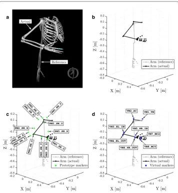
Fig. 1 Representations of the used upper limb model with reference poses and markers. a Screenshot taken
from OpenSim while displaying the used full arm model. The reference configuration is shown as a shaded
overlay on an actual example configuration determined by the joint angle vector [θelv=0◦, θsh_elv=63◦, θsh_rot=15◦, θel_flex=95◦, θpro_sup=−60◦, θdev_c=0◦, θflex_c=20◦]. b Representation of the
model’s exported structure in MATLAB producing the same actual configuration as in sub-figure (a) using
the developed forward kinematics function (functionally equivalent to OpenSim’s version). c Locations of
prototype markers that are solely used to the reconstruction of model-defined anatomical joint angles with
the proposed algorithm. d Locations of virtual markers that are used for the algorithm validation process by
Orthonormal bases
Shoulder The three independent model axes for the shoulder (defined in model bodies
humphant, humphant1 and humerus that have the same position), collectively denoted as Bsh_orig, were good candidates to form a basis because they are unit length vectors
(like all axes in the model) and almost orthogonal to each other (pairwise deviations from right angle are 0.00064°, 0.0029° and 0.0002°). For proper operation of the pro-posed algorithm however, these axes were orthogonalized using QR decomposition (see Appendix 2) to prevent error accumulation during the calculations. This resulted in the orthonormal basis Bsh_orth.
As a result, rotations in the shoulder can be expressed as elemental rotations of Bsh_orth
with acceptable angle errors due to the pairwise deviations between the original and new basis vectors after orthogonalization (0.000019°, 0.000655° and 0.002925°, respectively).
Elbow As relative orientation of the two rotation axes in the elbow is not close enough to orthogonal and the axes are defined in different parent bodies (rel_flex → ulna and rpro_sup → radius), the orthonormal basis Bpro_sup and the rotation matrix RBpro_sup
rel_flex(θel_flex) were formed to properly express the compound rotation as the
prod-uct of an axis-angle and an elementary rotation about the main axis in Bpro_sup. Again,
some angle errors are expected while calculating the elbow flexion angle in this basis because rel_flex is threated as it would belong to the radius body of the model.
Wrist Rotations in the wrist are the most complex among the three anatomical joints. Effects of the two active joint coordinates (deviation and flexion) are distributed among two model bodies (lunate and capitate), each having two nonorthogonal rotations (rdev ,
rflex→lunate and rpdr1, rpdr3→capitate) depending on both joint coordinates. To deal with the complexity of this structure, the orthonormal basis Bpdr3 and rotation axes rBpdr3
dev , r
Bpdr3 flex and r
Bpdr3
pdr1 were constructed to prepare the calculation of θdev and θflex. Using this approach, rdev and rflex are threated as if they would belong to the capitate
body of the model.
Marker placement
In order to add virtual markers to any OpenSim model, the parent body and the loca-tion within the parent’s frame have to be defined for each marker. Having the orthonor-mal bases from the previous section (Bsh_orth, Bpro_sup and Bpdr3), 12 prototype markers were placed on the model as follows (for reference, see Fig. 1c):
• Four markers were placed into each orthonormal basis having one at the origin of the actual basis ([0 0 0] in its parent body) and one in each axis of the basis.
• The markers were named using the convention PMx_[SH|EL|WR]_[O|X|Y|Z]
where PM refers to prototype marker, x is the serial number of the basis in which the marker is located (1–3), [SH|EL|WR] refers to the anatomical joint in which the marker is located and [O|X|Y|Z] refers to the marker’s location within the actual basis (origin or any of the axes). For example the name of the wrist’s origin marker is
PM3_WR_O.
markers reflect the compound rotation matrix in each anatomical joint (in the corre-sponding basis) at any time instant. To utilize this feature it is crucial that the struc-ture of each joint’s marker subset remains consistent during measurements (by keeping the formation of an orthonormal basis), because any deviation in relative marker posi-tions renders the derived compound rotation matrix inaccurate. As a consequence, it is recommended to use arm segment orientations to calculate the actual positions of prototype markers instead of measuring them directly. This can be achieved when using optical motion capture devices as segment orientations can be reconstructed with most systems by having at least three markers on each segment, however this is still an offline process. More importantly, utilizing orientation information makes the application of inertial sensors possible and beneficial in this setup as they are used to determine ori-entation directly. As an additional benefit, the offset-independent nature of oriori-entation information enables subject-independent joint angle reconstruction, rendering the scal-ing step of the standard inverse kinematics approach unnecessary in the process. Using this feature a real-time inverse kinematics algorithm is introduced in the next section that provides joint coordinate outputs coherent with OpenSim’s inverse kinematics tool.
Algorithm description
The key point in accelerating the selected upper limb model’s inverse kinematics calcula-tion is the model specific determinacalcula-tion of prototype marker locacalcula-tions. By construct-ing representative orthonormal bases in each anatomical joint of interest (Bsh_orth in
the shoulder, Bpro_sup in the elbow and Bpdr3 in the wrist) joint specific rotations can be addressed as elementary or axis-angle rotations in the corresponding bases. Having prototype markers in locations that reflect the actual orientations of these bases gives the possibility to express joint coordinates (rotation angles) in an efficient way, even in closed algebraic form in the shoulder and the elbow. As there was no closed form solu-tion found to calculate angles in the wrist, a numerical algorithm is given for this part of the problem. MATLAB R2015b (Mathworks, Natick, MA, USA) was used for algorithm prototyping and development.
Shoulder
Because shoulder prototype markers are placed on the model in a way that they show the actual orientations of the main axes of Bsh_orth, an experimental (numerical)
com-pound rotation matrix can be constructed from their spatial coordinates as shown in (1), where each marker position should be considered as a row vector.
By utilizing the kinematic structure of the shoulder joint (and keeping the assumption that Rshoulder =Rshoulder as detailed in Appendix 3), estimations of rotation angle values can be calculated as follows:
(1)
�
Rshoulder=
PM1_SH_XPM1_SH_Y−−PM1_SH_OPM1_SH_O PM1_SH_Z−PM1_SH_O Bsh_orth
T
(2a)
θsh_elv=arccos
Although the formulations in (2a) and (2c) could be susceptible to modulo π and sign
errors in general, the allowed angle ranges defined in the model (θsh_elv: 0◦→180◦, θsh_rot: −90◦→20◦) keep these equations safe to use until the experimental data does
not force the model outside of these ranges.
Elbow
Similarly to the shoulder, the experimental compound rotation matrix can be con-structed from the actual spatial positions of the elbow’s prototype markers. Because the model implements rotations in an incremental way, a reverse rotation of the extracted frame have to be performed in the shoulder’s basis to get the correct experimental rota-tion matrix for the elbow as shown in (3).
Having Relbow =Relbow estimations of joint angle values in the elbow can be calculated as (for further details, see Appendix 5):
where rBpro_sup
el_flex= [x y z]
As in the case of the shoulder, (4a) and (4b) should be used with care because of mod-ulo π and sign errors, but again having sufficient joint angle limits in the model (θel_flex
: 0◦→130◦, θpro
_sup: −90◦→90◦) application of these formulas is safe until
experi-mental data does not force the model outside of these ranges.
(2b)
θelv=atan2
Rshoulder(3,2) ,−R(shoulder1,2)
(2c)
θsh_rot=arcsin
ARshoulder(2,1) +BRshoulder(2,3) A2+B2
whereA=sin(θelv)sin(θsh_elv) and B=cos(θelv)sin(θsh_elv)
(3)
� Relbow =
PM2PM2__ELEL__YX−−PM2PM2__ELEL__OO PM2_EL_Z−PM2_EL_O
�Bsh_orthR�shoulderBTsh_orth �
Bpro_sup
T
(4a)
θel_flex=arccos
R(elbow1,1) −x2 1−x2
(4b)
θpro_sup=arcsin
AR(elbow1,2) +BRelbow(1,3)
A2+B2
A=ysinθel_flex
−xzcos(θel_flex)−1
B=zsin
θel_flex
+xy
cos(θel_flex)−1
Wrist
The experimental compound rotation matrix for the wrist can be constructed from the actual spatial positions of its prototype markers. Because of incremental rotations in the model, reverse rotations of the extracted frame have to be performed in the shoulder’s and elbow’s bases to get the correct experimental rotation matrix as shown in (5).
Although there is no closed form solution to calculate joint angle rotations in the wrist, the flexion angle can be determined as the solution of the following root finding problem (further details and definitions of a, b, c, x, y and z can be found in Appendix 7):
Based on this definition, the following properties hold for F(θflex,σ ):
1. (−θflex+η) defines a baseline with constant negative slope for the two possible solutions F(θflex,−1) and F(θflex, 1).
2. Because of the definition of the atan2(y,x) function, the value of atan2ξ−c2, c
will always be positive if ξ−c2 is real (i.e. c2≤ξ). This implies that the two solu-tions to F(θflex,σ ) do not cross the baseline but remain “below” (σ = −1) and “above” (σ =1) of it for all values of θflex.
As c depends on the actual compound rotation matrix Rwrist, its value is influenced by
both θdev_c and θflex_c. As a consequence, there may be wrist configurations where
c2> ξ for some regions of θflex, driving F(θflex,σ ) into a singular state within these regions. To prevent problems arising from this situation during the root finding process, singularity border points for θflex can be determined as follows. Let (7) as defined in (28), only θflex changed to ϑ to denote specific singularity border points.
Considering (6), singularity borders occur at locations where c2=ξ, resulting in c1,2= ±√ξ. Using these equalities and Euler’s formula, c can be rewritten into an expo-nential form that can be solved for ϑ resulting in the formulas shown below.
(5)
� Rwrist =
PM3_WR_XPM3_WR_Y−−PM3_WR_OPM3_WR_O PM3_WR_Z−PM3_WR_O
�Bsh_orthR�shoulderBTsh_orth �
·
�
Bpro_supR�elbowBpro_supT �
Bpdr3
T
(6)
GivenF(θflex,σ )= −θflex+η+σatan2
Reξ−c2, c,
where
η = atan2(b,a) σ ∈ {−1, 1}
ξ = a2+b2
findθflex=µsuch thatF(µ,σ )=0.
(7)
c=xcos(ϑ )+ysin(ϑ )+z
(8)
c1=
ξ:
ϑ1,2(1)= −ln √
ξ−z±ξ−2z√ξ−x2
−y2
+z2 x−iy
As a result, four separate complex-valued singularity border points can be determined for all wrist configurations. To get a better understanding of the structure of F(θflex,σ ) ,
the function was visually inspected with an interactive MATLAB script developed for this purpose. The tool allows the simulation of different user-defined wrist configura-tions through separate sliders for θdev_c and θflex_c while plotting all relevant
informa-tion about the problem (a representative screenshot is shown in Fig. 2). Based on manual testing throughout the model-defined ranges for θdev_c and θflex_c, the following
obser-vations were made:
1. The condition in (23) is always met.
2. ϑ1,2(k)((k=1)∨(k=2)) are separate real numbers if there is a singularity region in the actual wrist configuration for ck. In this case θflex=ϑ1(k) and θflex=ϑ2(k) indi-cate singularity border locations directly.
3. ϑ1,2(k)((k=1)∨(k=2)) are complex conjugates if there is no singularity region in the actual wrist configuration for ck. In this case θflex=Re
ϑ1(k)
=Re
ϑ2(k)
indi-cates the location where the values of F(θflex,−1) and F(θflex, 1) are closest to (k=1) and furthest from (k=2) each other.
4. Reϑ1,2(2)
always remain outside the model defined range of θflex.
5. θflex=η is the “gluing point” of F(θflex,−1) and F(θflex, 1), meaning that the singularity region for c1 starts to develop from this location, driving F(θflex,σ ) to
“stick” to the baseline.
6. If there is a singularity region for c1, Re
ϑ1(1)
remains always smaller than µ where F(µ,σ )=0.
(9)
c2= −
ξ:
ϑ1,2(2)= −ln
− √
ξ+z±ξ+2z√ξ−x2−y2+z2
x−iy
i
Fig. 2 Representative screenshot of the tool developed for visual inspection of F(θflex,σ ) [defined in (6)]. The interactive MATLAB script allows simulation of different user-defined wrist configurations through
sepa-rate sliders for θdev_c and θflex_c while plotting all relevant information about the optimization problem. The
7. In cases when the singularity region starts to develop (i.e. Im
ϑ1(k) is sufficiently small but not zero), two separate roots may appear, but only one being valid.
8. F(θflex,σ ) will have a valid root at θflex=µ if and only if σ =sign(µ−η).
Based on these observations, (6) can be solved with the following algorithm:
Algorithm 1:
Numerical algorithm to calculate
θ
flexData:
x, y, z, η
and
ξ
from (A.7.7) and (6)
Result:
θ
flex=
µ
such that
F
(
µ, σ
) = 0
1begin
2
calculate
ϑ
(1)1and
ϑ
(1)2from (8)
3
determine the interval [
ζ
1, ζ
2] in whichF
(
µ, σ
) changes sign
4
if
ϑ
(1)1−
ϑ
(1)2<
10
−10then
5
θ
flex←−
arg zero
µ∈[ζ1,ζ2]
F
(
µ,
1)
6
else
7
if
Re
ϑ
(1)1> η
then
8
θ
flex←−
arg zero
µ∈[ζ1,ζ2]
F
(
µ,
1)
9
else if
Re
ϑ
(1)1< η
then
10
θ
flex←−
arg zero
µ∈[ζ1,ζ2]
F
(
µ,
−
1)
11
else
12
θ
flex←−
η
13
end
14
end
15
end
Having the value of θflex, θflex_c and θdev_c can be calculated as follows:
where v1=expθflexrBpdr3 flex
rBpdr3
pdr1 and w1=
Rwristexp−θflex[1 0 0]
rBpdr3 flex.
Although the computational demand of wrist angle calculations is higher than of the shoulder and the elbow, the algorithm has still higher overall time efficiency than the optimization approach used by OpenSim’s inverse kinematics tool, as it is shown in the "Results" section.
(10a)
θflex_c=2∗θflex
(10b)
θdev_c=atan2
w1Tr1×v1,v1Tw1−
vT1r1
Algorithm validation
Testing and validation of the described algorithm was automated using OpenSim with its Python API and MATLAB. To make direct comparison possible between OpenSim’s optimization method and the proposed algorithm, eight additional virtual markers were placed on the model at locations that are suitable for optical motion capture (e.g. using Vicon) simulating an environment where OpenSim is generally applied. The virtual marker locations are the following (for visual reference, see Fig. 1d):
• VM1_TH : Thorax marker at the upper end of the sternum.
• VM2_AC : Acromio-clavicular joint of the shoulder girdle.
• VM3_EL_IN : Medial epicondyle of the humerus.
• VM4_EL_OUT : Lateral epicondyle of the humerus.
• VM5_WR_IN : Distal head of the radius.
• VM6_WR_OUT : Distal head of the ulna.
• VM7_MC2 : Distal head of the second metacarpal bone.
• VM8_MC5 : Distal head of the fifth metacarpal bone.
The structure of the upper limb model (including marker positions) was extracted using OpenSim’s Python API and saved into a .mat file for further processing with MATLAB. A forward kinematics function (functionally equivalent to OpenSim’s implementation) was developed in MATLAB to calculate body and marker positions for specific joint coordinate vectors of [θelv, θsh_elv, θsh_rot, θel_flex, θpro_sup, θdev_c, θflex_c] in the
model, enabling the analysis of trajectories for both PMx and VMx markers from artifi-cially generated movement patterns (Fig. 1b–d).
Simulated movement patterns
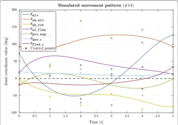
To avoid possible problems accompanying experimental measurements, simulated movement patterns were generated to test the performance and validity of the proposed algorithm. 100 separate pseudo-random (random seed = 10) joint coordinate trajecto-ries were constructed in MATLAB having a duration of 5 s and a sampling frequency of 100 Hz. The trajectories were generated as 5th order Bézier-curves as shown in (11) using six uniformly distributed control points (0, 20,...,100%) with randomly chosen val-ues for each joint coordinate from their valid intervals defined in the model. A repre-sentative movement pattern is shown in Fig. 3.
Following this step, forward kinematics was performed for each of the simulated pat-terns to calculate PMx and VMx marker trajectories yielding simulated “measurement” data as it would have been recorded during a real movement. The resulted trajectories were then used as inputs to inverse kinematics calculations with OpenSim (VMx) and
(11)
B5(t)= 5
i=0
5 i
ti(1−t)5−iPi
=(1−t)5P0+5t(1−t)4P1+10t2(1−t)3P2
+10t3(1−t)2P3+5t4(1−t)P4+t5P5
our algorithm (PMx) while the corresponding movement patterns served as reference for the outputs of each of the tested methods.
Inverse kinematics with OpenSim
To speed up the validation process, OpenSim (v3.3) was compiled from source on a Super-micro server having two Intel® Xeon® E5-2695 v3 CPUs (with a total of 56 execution threads) and 64 GB RAM, running Ubuntu Server 14.04.2 LTS operating system. Although the inverse kinematics (IK) algorithm in the used OpenSim version do not utilize multi-core architectures natively, each IK task can be divided into separate subtasks that can run in parallel thanks to the applied optimization method (there is no data dependency between time frames). To utilize this property, a pipeline was developed using MATLAB and Bash to prepare VMx marker data and the required files for OpenSim and manage file transfers, multi-threaded IK execution, results collection and evaluation. One important step before performing the IK calculation in OpenSim is subject-specific scaling of the used model and relative weighting of the markers. As only simulated data were used in the current study on an unmodified upper limb model, the scaled model file was identical to the original file during IK execution, while all marker weights were equal.
Algorithm implementation
The prototype of the proposed algorithm was implemented in MATLAB and tested with the simulated PMx marker trajectories. Calculation of (6) was performed using
Fig. 3 Representative simulated movement pattern used for algorithm validation. Simulated movement patterns were generated to validate the proposed kinematic algorithm. 100 separate pseudo-random joint coordinate trajectories were constructed as 5th order Bézier-curves having 5 s duration and 100 Hz sampling
frequency. PMx and VMx marker trajectories were calculated with our forward kinematics MATLAB function
MATLAB’s built-in fzero() function. Based on the MATLAB version, the algorithm was implemented in ANSI C to target practical applications. In this case (6) was solved with Brent’s root finding algorithm from [44]. Furthermore, compilation options were included to assess the effects of different data precisions (float or double) on the accuracy and execution time of the algorithm. This was not an option with MATLAB because fzero() cannot be used with float input.
To address possible accuracy problems arising from the lower precision of float data, an additional test case with a simple output continuity check for wrist angles was included, namely when the absolute difference between two successive θflex_c values is
larger than 5°, the actual θflex_c will be the previous θflex_c + 0.5°. This modified
ver-sion of the algorithm is denoted with mod. suffix among the results.
Evaluation platforms
MATLAB and C implementations of the proposed algorithm were tested on a sys-tem with an Intel® Core® i5-540M processor running Ubuntu Desktop 14.04.4 LTS. In
addition, the C implementation was evaluated on the following microcontroller units (MCUs) that are capable of targeting resource constrained environments (e.g. wearable measurement devices) with high performance:
1. STM32F407VG - ARM Cortex-M4 core with single precision floating point unit (FPU), up to 168 MHz core clock, 1 MB Flash memory, 192 KB SRAM.
2. STM32F746NG - ARM Cortex-M7 core with single precision FPU and L1-cache, up to 216 MHz core clock, 1 MB Flash memory, 320 KB SRAM.
For proper comparison, both MCUs were clocked at 168 MHz and the source codes dif-fered only in device specific details (e.g. hardware initialization). Algorithm evaluation on the MCUs was controlled with MATLAB via a UART link including data preparation, transmission and storage.
Performance metrics
To evaluate the overall performance of the algorithm compared to OpenSim’s IK method, accuracy and execution times were analyzed in all cases (OpenSim, MATLAB and C implementations). To assess accuracy, RMS values were computed for the differ-ences between the calculated and simulated joint coordinate trajectories for each trial. Means and standard deviations of these RMS values were then calculated across trials for each platform and precision (where this was applicable).
Running times of OpenSim’s IK evaluation were calculated as a sum of subtask execu-tion times from the IK log output directly. Algorithm execuexecu-tion times were measured by the tic and toc methods in MATLAB, the clock() function from the <time.h> library for the C implementation on PC and on-chip hardware timers clocked at 1 MHz for both MCUs.
Data exclusion from OpenSim trials
seemingly random locations in the IK output (independently of subtask borders men-tioned in "Inverse kinematics with OpenSim" section). This phenomenon may be han-dled by marker placement adjustment or error checking in measurement data in general. As IK input was strictly controlled by using simulated trajectories and the markers remained intact in the model between trials, further troubleshooting would have been needed to find a solution to this issue. Because the main emphasis of the study is the proposed algorithm and not OpenSim’s internal workings and IK troubleshooting, all OpenSim trials were excluded from final accuracy assessment where any of the resulted joint coordinate RMS errors exceeded 5° to not bias the results with incorrect data. As a result, only 59 trials out of 100 were used to calculate the accuracy of OpenSim’s IK algo-rithm. This however did not have any effect on the other measurements, so MATLAB and all C results were calculated across 100 trials.
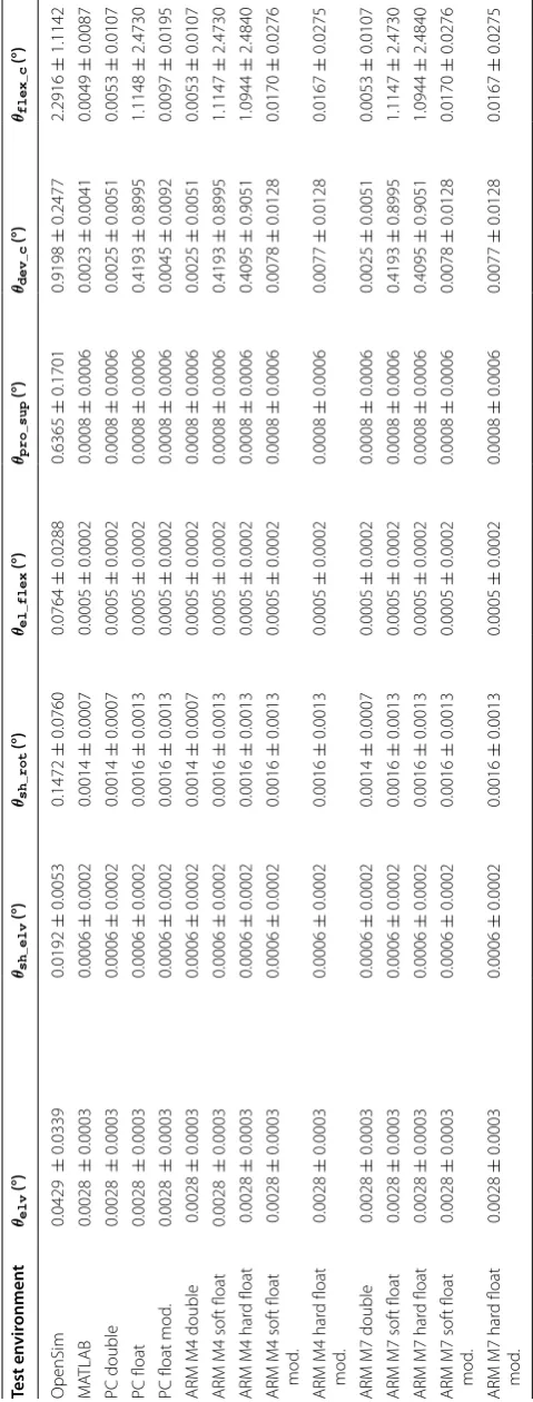
Results Accuracy
RMS errors from algorithm evaluation are shown in Table 1. The results show that con-sidering the mean of all valid trials (59 for OpenSim, 100 for all others), all platforms performed reasonably well producing errors below 3° for all joint coordinates (for a trial-wise visual comparison between OpenSim’s IK method and the proposed algorithm, see Additional file 3).
Regarding OpenSim it can be seen that errors for each joint coordinate are larger than those provided by our algorithm. The reason for this can lie in the optimization approach of OpenSim that in fact contains hard-coded convergence (0.0001) and iter-ation (1000) limits. However these limits prevent OpenSim’s IK algorithm to match the simulated movement patterns perfectly, they provide a practical solution to the accuracy↔running time trade-off for the software’s general usage.
MATLAB and C implementations of the proposed algorithm performed equally well for shoulder and elbow angles independent of the used data precision (double / float). This could occur because of the relatively low number of operations needed by these joint coordinates shown in equation groups () and () that prevented considerable error accumulation due to the lower precision of float. Regarding wrist angles a clear dis-tinction can be made between double and float (MATLAB uses double as default). The two main reasons for this phenomenon are (1) the significantly larger computational demand of θdev_c and θflex_c involving iterative processes that can lead to precision
Table 1 RMS err ors Each r ow r epr esen
ts a separ
at e t est en vir onmen t f
or the r
ef
er
enc
e (
OpenSim) and pr
oposed in verse k inema tics algor ithm. The c olumns sho w mean ± standar d deviation join
t angle RMS er
rors acr
oss all v
alid tr
ials (59 f
or
OpenSim, 100 other
wise) f
or each t
est en vir onmen t Test en vir onmen t θe l v (°)
θsh
_
e
l
v
(°)
θsh
_
r
o
t
(°)
θel
_ f l e x (°)
θpr
o _ s u p (°)
θde
v _ c (°) θf l ex _ c (°) OpenSim 0.0429 ± 0.0339 0.0192 ± 0.0053 0.1472 ± 0.0760 0.0764 ± 0.0288 0.6365 ± 0.1701 0.9198 ± 0.2477 2.2916 ± 1.1142 M ATLAB 0.0028 ± 0.0003 0.0006 ± 0.0002 0.0014 ± 0.0007 0.0005 ± 0.0002 0.0008 ± 0.0006 0.0023 ± 0.0041 0.0049 ± 0.0087 PC double 0.0028 ± 0.0003 0.0006 ± 0.0002 0.0014 ± 0.0007 0.0005 ± 0.0002 0.0008 ± 0.0006 0.0025 ± 0.0051 0.0053 ± 0.0107 PC float 0.0028 ± 0.0003 0.0006 ± 0.0002 0.0016 ± 0.0013 0.0005 ± 0.0002 0.0008 ± 0.0006 0.4193 ± 0.8995 1.1148 ± 2.4730
PC float mod
. 0.0028 ± 0.0003 0.0006 ± 0.0002 0.0016 ± 0.0013 0.0005 ± 0.0002 0.0008 ± 0.0006 0.0045 ± 0.0092 0.0097 ± 0.0195
ARM M4 double
0.0028 ± 0.0003 0.0006 ± 0.0002 0.0014 ± 0.0007 0.0005 ± 0.0002 0.0008 ± 0.0006 0.0025 ± 0.0051 0.0053 ± 0.0107
ARM M4 sof
t float 0.0028 ± 0.0003 0.0006 ± 0.0002 0.0016 ± 0.0013 0.0005 ± 0.0002 0.0008 ± 0.0006 0.4193 ± 0.8995 1.1147 ± 2.4730
ARM M4 har
d float 0.0028 ± 0.0003 0.0006 ± 0.0002 0.0016 ± 0.0013 0.0005 ± 0.0002 0.0008 ± 0.0006 0.4095 ± 0.9051 1.0944 ± 2.4840
ARM M4 sof
t float mod . 0.0028 ± 0.0003 0.0006 ± 0.0002 0.0016 ± 0.0013 0.0005 ± 0.0002 0.0008 ± 0.0006 0.0078 ± 0.0128 0.0170 ± 0.0276
ARM M4 har
d float mod . 0.0028 ± 0.0003 0.0006 ± 0.0002 0.0016 ± 0.0013 0.0005 ± 0.0002 0.0008 ± 0.0006 0.0077 ± 0.0128 0.0167 ± 0.0275
ARM M7 double
0.0028 ± 0.0003 0.0006 ± 0.0002 0.0014 ± 0.0007 0.0005 ± 0.0002 0.0008 ± 0.0006 0.0025 ± 0.0051 0.0053 ± 0.0107
ARM M7 sof
t float 0.0028 ± 0.0003 0.0006 ± 0.0002 0.0016 ± 0.0013 0.0005 ± 0.0002 0.0008 ± 0.0006 0.4193 ± 0.8995 1.1147 ± 2.4730
ARM M7 har
d float 0.0028 ± 0.0003 0.0006 ± 0.0002 0.0016 ± 0.0013 0.0005 ± 0.0002 0.0008 ± 0.0006 0.4095 ± 0.9051 1.0944 ± 2.4840
ARM M7 sof
t float mod . 0.0028 ± 0.0003 0.0006 ± 0.0002 0.0016 ± 0.0013 0.0005 ± 0.0002 0.0008 ± 0.0006 0.0078 ± 0.0128 0.0170 ± 0.0276
ARM M7 har
Execution time
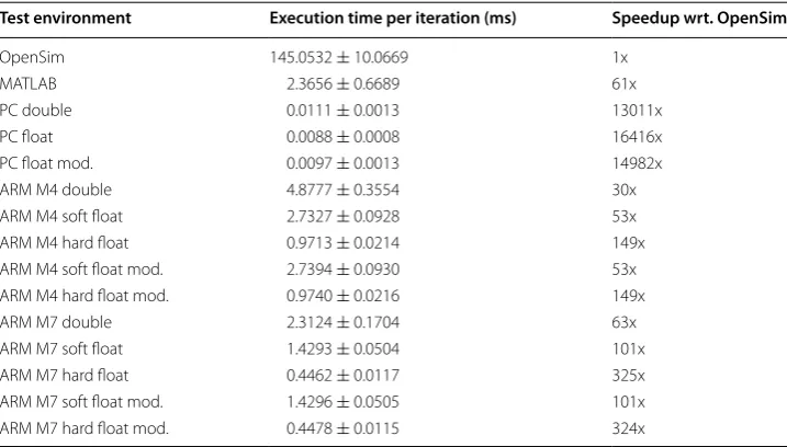
To assess overall performance, execution times were compared between OpenSim’s IK method and our proposed algorithm on different platforms and are shown in Table 2.
Measurement results show that the optimization approach of OpenSim performed the calculation of a single iteration in 145 ms on average. Because of the application specific nature of the proposed algorithm, its running times considering different implementa-tions (MATLAB/C), data precisions (double/float) and platforms (PC/ARM Cortex-M) all showed a significant increase in execution performance compared to OpenSim, the worst result being about 5 ms on average for a single iteration.
As expected, the C implementation is more than two orders of magnitude faster than the MATLAB version on the PC, yielding execution times per iteration about 10 μs with all precision variants (double, float and float mod.). Opposed to this, running times on embedded platforms showed more scattered results. The difference between
double and float is more expressed in these cases while application of the FPU accel-erates float computations even further (hard float entries in Table 2). Regarding the modified algorithm variant it can be seen that even the extra continuity check adds some amount to the execution time per iteration, the possibility to use float precision brings more speed advantage, especially with the FPU enabled. These findings are true for both tested MCUs with the observation that ARM’s M7 architecture is about twice as fast as M4 when running the presented algorithm with the same core clock.
Discussion
Evaluation results of the tested algorithms show that each approach provides proper accuracy for most common arm movement analysis scenarios. One important aspect however is that while OpenSim provides a useful general tool for biomechanical analy-sis including fields beyond inverse kinematics (e.g. inverse and forward dynamics), the
Table 2 Execution times
Each row represents a separate test environment for the reference (OpenSim) and proposed inverse kinematics algorithm. Table values show mean ±standard deviation for a single iteration across all valid trials (59 for OpenSim, 100 otherwise) and the speed increase of each tested setup with respect to OpenSim
Test environment Execution time per iteration (ms) Speedup wrt. OpenSim
OpenSim 145.0532 ± 10.0669 1x
MATLAB 2.3656 ± 0.6689 61x
PC double 0.0111 ± 0.0013 13011x
PC float 0.0088 ± 0.0008 16416x
PC float mod. 0.0097 ± 0.0013 14982x
ARM M4 double 4.8777 ± 0.3554 30x
ARM M4 soft float 2.7327 ± 0.0928 53x
ARM M4 hard float 0.9713 ± 0.0214 149x
ARM M4 soft float mod. 2.7394 ± 0.0930 53x
ARM M4 hard float mod. 0.9740 ± 0.0216 149x
ARM M7 double 2.3124 ± 0.1704 63x
ARM M7 soft float 1.4293 ± 0.0504 101x
ARM M7 hard float 0.4462 ± 0.0117 325x
ARM M7 soft float mod. 1.4296 ± 0.0505 101x
calculation of joint angles from the actual experimental data is rather demanding com-putationally. As the output of this step gives the basis for all other analysis methods in the software, the amount of time needed for the overall processing pipeline highly depends on the efficiency of this algorithm. As Table 2 shows, the average amount of time needed for OpenSim’s IK algorithm to perform a single iteration would allow about 7 Hz operation that falls behind the generally accepted practice in human movement recording of at least 50 Hz. This property excludes OpenSim from tight integration with systems requiring real-time movement kinematics, however that is not the software’s original target application anyway (up to version 3.3 at least).
Considering the algorithm proposed in the study Tables 1 and 2 show a significant improvement in performance in both accuracy and execution time when compared to OpenSim’s IK method. The main reason for this difference is the algorithm’s applica-tion specific nature with the utilizaapplica-tion of both the internal structure of the used upper limb model and inertial sensing of movement to determine limb segment orientations directly. As the MATLAB version showed proper accuracy and sufficiently short exe-cution time on the PC, implementation of the algorithm in ANSI C was reasonable to assess its “real” performance without the overhead of a general prototyping tool that MATLAB essentially has. Because accuracy results are the same or very similar across specific variants of the C implementation (i.e. using double/float precision), only exe-cution time differences are discussed later in the text.
Running times of the algorithm’s C implementation showed more than four orders of magnitude speedup on the tested Intel® Core® i5-540M processor compared to
Open-Sim’s IK algorithm on a more recent and higher performance server CPU with Xeon® architecture, yielding about 10 μs execution time per iteration for all variants. How-ever this is an impressive improvement, running the algorithm on PC would still pose problems from practical aspects of possible applications (e.g. total size and mobility of the measurement system or communication overhead between the measuring and pro-cessing device), so the real benefit of this speed increase lies in the “spare” performance that opened the way to testing the algorithm in resource constrained embedded envi-ronments. Evaluation of the proposed method on high performance MCUs showed that all implementation variants that provided good accuracy (double and [soft/hard] float mod.) had acceptable execution times on both architectures (M4 and M7) for real-time operation, considering 100 Hz as sufficient sampling frequency for human movement analysis. Based on these results, the specific implementation variant should be chosen taking the overall design requirements of the actual practical application into account (i.e. wearable measurement devices like the one presented in [45]) as in most cases the algorithm should fit into a system containing other computationally demand-ing processes (like sensor fusion algorithms) with power consumption bedemand-ing a critical part of the design for example.
It needs to be emphasized however that the application specific nature of the algo-rithm and its dependency on the used upper limb model induce some practical con-siderations, because having a method that works in a strictly controlled simulation environment does not guarantee its applicability in a real situation. A fundamental thing to consider is whether data provided by real sensors reflect arm segment orientations needed by the algorithm accurately. As this was a key requirement from the beginning of algorithm design, the prototype markers were defined in local bases of the joints that can be directly expressed in terms of sensor orientations (for details, see Additional files 1, 2). As an additional benefit, the definition of an anatomical calibration proce-dure—often needed when inertial sensors are used for human movement recording— can be avoided as the proposed algorithm does not use segment length information for joint angle reconstruction. What cannot be avoided however is the accurate estimate of sensor orientations, as the whole process depends highly on the precision of this step. Although there is no ultimate solution to the problem of inertial sensor fusion yet, there are continuous algorithmic efforts to reach higher accuracy and reliability (for differ-ent highlighted approaches, see "Background" section). But even in cases when the sen-sors provide accurate orientation information of the measured limb, care must be taken when determining the limb’s reference orientation based on the measurements. The rea-son for this is mainly inter-subject variability in the sense that even the model defines the reference posture clearly, it cannot be assumed that any actual subject will repro-duce the same posture very accurately that can lead to offset errors during the meas-urement. Furthermore, the assumption was made during algorithm development that the measured movement always remains within the valid joint angle ranges defined in the model. As long as this assumption holds (as in the case of simulated movement pat-terns presented in this study), the algorithm should not have problems with proper joint angle reconstruction. However, if outliers are present in the experimental data (e.g. ref-erence posture errors, inaccuracies in the measurement or the sensor fusion algorithm or extreme anatomical ranges of a subject) undefined output states can occur. This may be handled with a simple saturation technique on the algorithm level but rather should be prevented by applying proper experimental design and calibration methods. In a practical setup this involves proper sensor placement and various steps before the meas-urements including zero motion offset compensation, hard and soft iron error compen-sation in the magnetometer and determining relative sensor orientations with respect to the measured segments [46, 47] for example.
Conclusions
providing the possibility to perform this step even on the measurement device in cases when accurate inertial movement sensing is applicable.
Abbreviations
LoS: line of sight; MEMS: micro-electro-mechanical system; IMU: inertial measurement unit; API: application program-ming interface; IK: inverse kinematics; XML: extensible markup language; ANSI: American National Standards Institute; MCU: microcontroller unit; FPU: floating point unit; PC: personal computer; RMS: root mean square.
Authors’ contributions
Both authors prepared the study and interpreted the results. In addition, BJB developed the mathematical background, designed and implemented the software components required for the validation of the proposed algorithm and drafted the manuscript. Both authors revised the manuscript and gave their final approval for publication. Both authors read and approved the final manuscript.
Acknowledgements
The authors would like to sincerely thank Endre László for his technical assistance and for proof reading the manuscript. Competing interests
The authors declare that they have no competing interests. Availability of data and materials
All data generated or analyzed during this study are included in this published article and its supplementary information files.
Funding
This work was financially supported by the Central Funding Program of Pázmány Péter Catholic University under project number KAP15-055-1.1-ITK.
Appendices
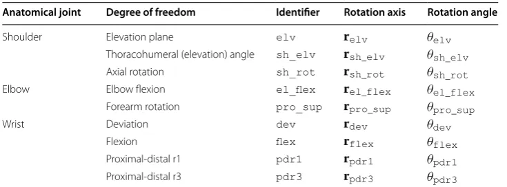
Appendix 1: Definitions
To facilitate algorithm description in the text, notations in Table 3 will be used to iden-tify each degree of freedom and the rotation axes and angle values for them, where each rotation axis (raxis_id) should be considered as a row vector.
Furthermore, the following definitions are introduced:
Additional files
Additional file 1. OpenSim version of the used upper limb model. Additional file 2. Marker sets defined for the study.
Additional file 3. Joint angle reconstruction figures for all simulated trajectories.
Table 3 Axis and angle notations
The table lists identifiers derived from the model file and notations of rotation axes and angles for all relevant degrees of freedom used for algorithm formulation
Anatomical joint Degree of freedom Identifier Rotation axis Rotation angle
Shoulder Elevation plane elv relv θelv
Thoracohumeral (elevation) angle sh_elv rsh_elv θsh_elv
Axial rotation sh_rot rsh_rot θsh_rot
Elbow Elbow flexion el_flex rel_flex θel_flex
Forearm rotation pro_sup rpro_sup θpro_sup
Wrist Deviation dev rdev θdev
Flexion flex rflex θflex
Proximal-distal r1 pdr1 rpdr1 θpdr1
1. An orthonormal basis with a selected rotation axis in its main axis will be noted as
Baxis_id_0, where axis_id_0 is the identifier of the axis (e.g. for a basis with relv in its main axis the basis will be Belv). If the basis is not formed by orthogonalization
of rotation vectors in the model (as in the case of the shoulder), Baxis_id_0 is defined
as
2. The rotation axis raxis_id expressed in the basis Baxis_id_0 is defined as
3. Given a unit length vector r∈R3, Rodrigues’ formula gives the rotation matrix about
r of an arbitrary angle θ ∈ [−π,π[ as
4. The matrix representation of an axis-angle rotation formed from a unit axis raxis_id
and angle θaxis_id expressed in the basis Baxis_id_0 is given as follows:
where rBaxis_id_0
axis_id = [x y z], s=sin
θaxis_id
, c=cosθaxis_id
and C=1−C. 5. The ith element of vector v is denoted as v(i). Similarly, the (i, j)th element of matrix
R is denoted as R(i,j), where i is the row index and j is the column index. Indexing complete rows and columns is denoted as R(i,:) and R(:,j), respectively.
Appendix 2: QR orthogonalization
The general formula of QR orthogonalization is shown below, where A is a regular matrix, Q is an orthogonal matrix, R is an upper triangular matrix, S is the sign diagonal matrix of R and B is the resulting orthogonal matrix.
(12a)
Baxis_id_0=
raxisr_2id_0 r3
T
where
(12b)
r2=
raxis_id_0×raxis_id_0− [1 0 0]
raxis_id_0×
raxis_id_0− [1 0 0]
and
(12c)
r3= raxis_id_0×r2 raxis_id_0×r2
(13)
rBaxis_id_0
axis_id =raxis_idBaxis_id_0
(14)
expθr=I3+sin(θ )r+(1−cos(θ ))r2
where r:R3→R3 def= r v=r×v
(15)
RBaxis_id_0
raxis_id (θaxis_id)=exp
�
θaxis_id�r
Baxis_id_0
axis_id �
≡
yxCxxC++zs yyCc xyC−+zs xzCc yzC+−xsys
zxC−ys zyC+xs zzC+c
(16)
A=QR
(17)
S=
sii=1 ifrii>0
sii= −1 ifrii<0
Appendix 3: Auxiliary calculations for the shoulder
The orientation of the humerus is determined by four consecutive rotations in the shoul-der in the orshoul-der of elevation plane, elevation angle, -elevation plane and axial rotation degrees of freedom (for axis and angle notations, see Table 3). Based on axis definitions in the model, rotations about relv and rsh_rot can be estimated with an elementary
rota-tion about the second axis of Bsh_orth while the estimation of the rotation about rsh_elv
can be done with an elementary rotation about Bsh_orth’s third axis as shown in ().
Using these definitions, the symbolic expression of the compound rotation matrix that represents the actual orientation in the shoulder can be calculated as shown in (20). For the convenience of calculation, this step was performed with MATLAB’s Symbolic Math Toolbox using the script shown in Appendix 4.
where A=cos(θsh_elv)cos2(θelv)+sin2(θelv), B=(1−cos(θsh_elv))cos(θelv)sin(θelv), and C=cos(θsh_elv)sin2(θelv)+cos2(θelv).
(18)
B=QS
(19a)
RBrelvsh_orth(θelv) =
cos(θ0elv) 0 sin1 (θ0elv)
−sin(θelv) 0 cos(θelv)
(19b)
RBrshsh_orth_rot(θsh_rot) =
cos(θsh0_rot) 0 sin1 (θsh0_rot)
−sin(θsh_rot) 0 cos(θsh_rot)
(19c)
RBrshsh_orth_elv(θsh_elv) =
cos(θshsin(θsh__elv)rot) −cos(θshsin(θsh_rot)_elv) 00
0 0 1
(20)
Rshoulder
=RBsh_orth
relv (θelv)Rrsh_elv(θshBsh_orth _elv)RrelvBsh_orth(−θelv)RBrsh_rot(θshsh_orth _rot)
=
Acos(θsh_rot)−Bsin(θsh_rot) −cos(θelv)sin(θsh_elv) Asin(θsh_rot)+Bcos(θsh_rot)
sin(θelv)sin(θsh_elv)sin(θsh_rot) cos(θsh_elv) cos(θelv)sin(θsh_elv)sin(θsh_rot) +cos(θelv)sin(θsh_elv)cos(θsh_rot) −sin(θelv)sin(θsh_elv)cos(θsh_rot)
Bcos(θsh_rot)−Csin(θsh_rot) sin(θelv)sin(θsh_elv) Bsin(θsh_rot)+Ccos(θsh_rot)
Appendix 4: MATLAB code for the compound rotation matrix of the shoulder
% anonymous function to generate rotation matrix about the second axis of % the actual basis
R_2nd =@(theta) [ cos(theta) 0 sin(theta) ;
0 1 0 ;
-sin(theta) 0 cos(theta)];
% anonymous function to generate rotation matrix about the third axis of % the actual basis
R_3rd =@(theta) [cos(theta) -sin(theta) 0 ; sin(theta) cos(theta) 0 ;
0 0 1];
% symbolic variables for the joint coordinates (rotation angles) syms elv_angle shoulder_elv shoulder_rot;
% generate the individual rotation matrices R_elv_angle = R_2nd(elv_angle);
R_shoulder_elv = R_3rd(shoulder_elv); R_elv_angle_minus = R_2nd(-elv_angle); R_shoulder_rot = R_2nd(shoulder_rot);
% calculate the compound rotation matrix
R_shoulder = R_elv_angle * R_shoulder_elv * R_elv_angle_minus * R_shoulder_rot;
Appendix 5: Auxiliary calculations for the elbow
The orientation of the forearm is defined by two consecutive rotations in the order of elbow flexion and forearm rotation. If expressed in Bpro_sup, the rotation matrix about
rel_flex can be estimated as RBpro_sup
rel_flex(θel_flex) while rotation about rpro_sup
cor-responds to the elementary rotation about the first axis of Bpro_sup [denoted as RBpro_sup
rpro_sup(θpro_sup)]. Multiplication of these matrices yields the compound rotation matrix in the elbow as shown in (21) (the corresponding MATLAB script can be found in Appendix 6).
(21)
Relbow=RBrel_flexpro_sup(θel_flex)R
Bpro_sup
rpro_sup(θpro_sup)
=
�
1−cos(θel_flex)
�
x2+ Asin(θpro_sup)− Acos(θpro_sup)+
cos(θel_flex) Bcos(θpro_sup) Bsin(θpro_sup) zsin(θel_flex)− Dcos(θpro_sup)− −Dsin(θpro_sup)−
C Esin(θpro_sup) Ecos(θpro_sup) −ysin(θel_flex)− Gsin(θpro_sup)+ Gcos(θpro_sup)−
F Hcos(θpro_sup) Hsin(θpro_sup)
where
relBpro_sup_flex = [x y z]
A = ysin(θel_flex)−F B = zsin(θel_flex)+C C = xy�cos(θel_flex)−1
�
D = �1−cos(θel_flex)
�
y2+cos(θel_flex) E = xsin(θel_flex)+yz
�
cos(θel_flex)−1
�
F = xz�cos(θel_flex)−1
�
G = �1−cos(θel_flex)
�
z2+cos(θel_flex) H = xsin(θel_flex)−yz
�
cos(θel_flex)−1
Appendix 6: MATLAB code for the compound rotation matrix of the elbow
% anonymous function to generate rotation matrix about the first axis of % the actual basis
R_1st =@(theta) [1 0 0 ;
0 cos(theta) -sin(theta) ;
0 sin(theta) cos(theta)];
% symbolic variables for axis coordinates (spatial) and % joint coordinates (rotation angles)
syms x y z elbow_flexion pro_sup;
% auxiliary variables for the axis-angle rotation matrix c = cos(elbow_flexion);
s = sin(elbow_flexion); C = 1 - c;
% generate the individual rotation matrices R_pro_sup = R_1st(pro_sup);
R_elbow_flexion = [x*x*C+c , x*y*C-z*s , x*z*C+y*s ;
y*x*C+z*s , y*y*C+c , y*z*C-x*s ;
z*x*C-y*s , z*y*C+x*s , z*z*C+c ];
% calculate the compound rotation matrix R_total = R_elbow_flexion * R_pro_sup;
Appendix 7: Auxiliary calculations for the wrist
The orientation of the hand is defined in the model by four consecutive rotations in the order of deviation, flexion, proximal-distal r1 and proximal-distal r3. Although deviation and flexion are used here as intermediate rotations, naming convention of actively con-trolled joint coordinates and intermediate rotations is inconsistent in the model file at this point because active joint coordinates of the wrist are called deviation and flexion, too. To prevent ambiguity, angle values of controlled joint coordinates of the wrist will be denoted as θdev_c and θflex_c further in the text. Intermediate wrist rotations are
distributed among two rows of carpal bones with different rotation angles depending on the actual values of θdev_c and θflex_c as follows:
1. Deviation and flexion are defined in the lunate body with rotation angle values of
θdev = θdev_c and θflex = 0.5∗θflex_c.
2. Proximal-distal r1 and proximal-distal r3 are defined in the capitate body with rota-tion angle values of θpdr1 = 1.5∗θdev_c if θdev_c is negative and θpdr1 = θdev_c
oth-erwise, and θpdr3 = 0.5∗θflex_c.
3. The angle limits for the controlled coordinates are: θdev_c∈ [−10◦, 25◦] and
θflex_c∈ [−70◦, 70◦].
If expressed in Bpdr3, the rotation matrices about rdev and rflex can be estimated as
RBpdr3
rdev (θdev) and R
Bpdr3
rflex(θflex), while rotation matrices for rpdr1 and rpdr3 can be expressed as RBpdr3
denoted by RBpdr3
rpdr3(θpdr3). Similarly to the shoulder and elbow joints, the compound
rotation matrix in the wrist can be written as follows:
One difficulty however is that this formulation contains three axis-angle rotations out of four that makes Rwrist a very complex symbolic expression with no closed form algebraic solution for the individual rotation angle values.
This problem was handled using a decomposition approach from the literature. As it is shown by Piovan and Bullo in [48], three Euler angles about arbitrary axes can be deter-mined from a rotation matrix if the rotation axes are known and the following condition is fulfilled:
where R is the rotation matrix and {r1,r2,r3} are the column vector rotation axes. If we assume that r1, r2, r3 and R satisfy (23), Euler angle values {θ1,θ2,θ3} can be calculated as follows:
• θ2 is one of the two solutions to
where a= −rT1r22r3, b=rT1r2r3 and c=rT1R−I3−r22
r3.
• if RTr1�= ±r3, then the angles θ1 and θ3 are uniquely determined by
where v1=expθ2r2r3, w1=Rr3, v3=exp−θ2r2r1, w3=RTr1.
As the inverse of any rotation matrix equals its transpose and the model defines the equality of θflex=θpdr3, (22) can be rewritten into
Having Rwrist=Rwrist, (24) can be used to express θflex from (27) as follows (all r
Baxis_id_0 axis_id here are considered as column vectors):
(22)
Rwrist =RBpdr3
rdev (θdev)R
Bpdr3
rflex(θflex)R
Bpdr3
rpdr1(θpdr1)R
Bpdr3
rpdr3(θpdr3)
(23)
r1T
R−r2rT2
r3
≤
1−rT1r22
1−r3Tr22
(24)
(θ2)1,2=atan2(b,a)±atan2
a2+b2−c2, c
(25)
θ1= atan2
w1Tr1×v1,v1Tw1−vT1r1w1Tr1
(26)
θ3= −atan2
w3Tr3×v3,v3Tw3−
vT3r3
w3Tr3
(27)
Rwrist
10 cos(θ0flex) sin(θ0flex)
0 −sin(θflex) cos(θflex)
=RBpdr3
rdev (θdev)R
Bpdr3
rflex(θflex)R
Bpdr3
![Fig. 2 Representative screenshot of the tool developed for visual inspection of The interactive MATLAB script allows simulation of different user-defined wrist configurations through sepa-rate sliders for two F(θflex, σ) [defined in (6)]](https://thumb-us.123doks.com/thumbv2/123dok_us/9116891.1904515/11.595.118.479.485.678/representative-screenshot-developed-inspection-interactive-simulation-different-configurations.webp)