The SPAtial EFficiency metric (SPAEF): multiple-component evaluation of spatial patterns for optimization of hydrological models

https://doi.org/10.5194/gmd-11-1873-2018 © Author(s) 2018. This work is distributed under the Creative Commons Attribution 4.0 License.

The SPAtial EFficiency metric (SPAEF): multiple-component

evaluation of spatial patterns for optimization

of hydrological models

Julian Koch1, Mehmet Cüneyd Demirel1,2, and Simon Stisen1

1_{Department of Hydrology, Geological Survey of Denmark and Greenland, Copenhagen, 1350, Denmark} 2_{Department of Civil Engineering, Istanbul Technical University, 34469 Maslak, Istanbul, Turkey} Correspondence:Julian Koch ([email protected])

Received: 9 October 2017 – Discussion started: 23 November 2017

Revised: 29 January 2018 – Accepted: 17 April 2018 – Published: 15 May 2018

Abstract. The process of model evaluation is not only an integral part of model development and calibration but also of paramount importance when communicating modelling results to the scientific community and stakeholders. The modelling community has a large and well-tested toolbox of metrics to evaluate temporal model performance. In con-trast, spatial performance evaluation does not correspond to the grand availability of spatial observations readily avail-able and to the sophisticate model codes simulating the spa-tial variability of complex hydrological processes. This study makes a contribution towards advancing spatial-pattern-oriented model calibration by rigorously testing a multiple-component performance metric. The promoted SPAtial EFfi-ciency (SPAEF) metric reflects three equally weighted com-ponents: correlation, coefficient of variation and histogram overlap. This multiple-component approach is found to be advantageous in order to achieve the complex task of com-paring spatial patterns. SPAEF, its three components indi-vidually and two alternative spatial performance metrics, i.e. connectivity analysis and fractions skill score, are applied in a spatial-pattern-oriented model calibration of a catch-ment model in Denmark. Results suggest the importance of multiple-component metrics because stand-alone metrics tend to fail to provide holistic pattern information. The three SPAEF components are found to be independent, which al-lows them to complement each other in a meaningful way. In order to optimally exploit spatial observations made avail-able by remote sensing platforms, this study suggests apply-ing bias insensitive metrics which further allow for a com-parison of variables which are related but may differ in unit. This study applies SPAEF in the hydrological context using

the mesoscale Hydrologic Model (mHM; version 5.8), but we see great potential across disciplines related to spatially distributed earth system modelling.

1 Introduction

Spatially distributed models, which represent various compo-nents of the earth system, are extensively applied in policy-making, management and research. Such modelling tackles a wide range of environmental problems, such as the anal-ysis of drought patterns (Herrera-Estrada et al., 2017), as-sessing the spatial regularization of fertilizers in agricultural landscapes (Refsgaard et al., 2014) or modelling vegetation dynamics (Ruiz-Pérez et al., 2016). Our study focuses on drological variability as predicted by spatially distributed hy-drological models. The correct representation of the spatial variability of hydrological fluxes often constitutes the major obstacle for many modelling efforts with respect to model structure, parameterization and forcing data.

1874 J. Koch et al.: The SPAtial EFficiency metric (SPAEF)

temporal model performance, but the call for a paradigm shift towards a spatial-pattern-oriented model evaluation using in-dependent spatial observations has been ongoing for nearly 2 decades (Grayson and Blöschl, 2001; Koch et al., 2016a; Stisen et al., 2011; Wealands et al., 2005). Modelling the temporal dynamics of hydrological response can be consid-ered independent of a model’s spatial component as different parameters control spatial and temporal variability (Pokhrel and Gupta, 2011). Along the lines of Gupta et al. (2008), the feasibility of an adequate spatial-pattern-oriented model evaluation is constrained by the versatility of the applied per-formance metric. The task to quantitatively compare spatial patterns is non-trivial and the multi-layered content of spa-tial patterns expresses distinct requirements to such a met-ric (Cloke and Pappenberger, 2008; Gilleland et al., 2009; Vereecken et al., 2016). A single metric will generally not ad-equately address performance and instead a combination of metrics spanning multiple relevant aspects of model perfor-mance are necessary (Clark et al., 2011; Gupta et al., 2012). The advantages of using multiple-component metrics have been broadly accepted for the evaluation of temporal model performance (Kling et al., 2012), but multiple-component evaluation has not yet been highlighted for the evaluation of simulated spatial patterns.

Model evaluation targeted at spatial performance requires reliable spatial observations which are broadly facilitated by remote sensing platforms across various spatial scales (Mc-Cabe et al., 2008; Orth et al., 2017). At a small scale, Glaser et al. (2016) explored the applicability of portable thermal in-frared cameras to evaluate simulated spatial patterns of sur-face saturation in the hillslope–riparian–stream intersur-face. At the catchment scale, Schuurmans et al. (2011) incorporate remote-sensing-based maps of latent heat in order to identify structural model deficiencies. At a regional scale, Mendig-uren et al. (2017) applied a spatial-pattern-oriented model evaluation based on remote sensing estimates of evapotran-spiration to diagnose shortcomings of the national hydrolog-ical model of Denmark. At a large scale, Koch et al. (2016b) utilized land surface temperature retrievals to evaluate large-scale land surface models across the continental US.

The applicability of remote sensing data to calibrate hy-drological models has already been explored by several stud-ies that incorporated spatial patterns of land surface tem-perature (Stisen et al., 2018), snow cover (Terink et al., 2015) or latent heat (Immerzeel and Droogers, 2008). Over-all the merit of constraining model parameters against spatial observations has been widely recognized by the modelling community. However, the design of the performance metric, which ensures that the spatial information contained in the remote sensing data is utilized optimally to inform the model calibration, is rarely touched upon in the literature.

Bennett et al. (2013) provide an excellent overview of measures that allow the modeller to quantify the performance of environmental models. They considered model evaluation a vital step during the iterative process of model

develop-ment, and hence it can identify the need for additional data, alternative calibrations or updated model structure. This fur-ther emphasizes the need for robust performance metrics. In general, the properties of the applied metric and the design of the evaluation framework should always correspond to the application of the model (Krause et al., 2005).

Our study highlights the development and application of a versatile metric that has the potential to advance the credi-bility of spatially distributed hydrological models. When de-signing such a metric it is important to reflect on require-ments as well as frameworks to properly test it in, which has been extensively discussed in the literature (Cloke and Pappenberger, 2008; Moriasi et al., 2007; Dawson et al., 2007; Krause et al., 2005; Refsgaard and Henriksen, 2004; Schaefi and Gupta, 2007). Following these references and our own reflections we identified the following five major requirements of a spatial performance metric: (1) the met-ric should be easy to compute, which makes results repro-ducible and creates credibility within the scientific commu-nity. (2) In order to be informative during model calibration the metric should be robust and deliver a continuous response to changes in parameter values. (3) In the formulation of the metric, multiple independent components are necessary to provide a holistic evaluation of the model performance. (4) The metric should offer the possibility to compare related variables of different units; e.g. observed latent heat (W m−2) and simulated evapotranspiration (mm day−1). This enables evaluation via proxies and facilitates bias insensitivity, which is found favourable because it focuses on the pattern informa-tion contained in the remote sensing data instead of absolute values at the grid scale. (5) The metric should be easy to com-municate both inside and outside the scientific community. This requires a predefined range and the possibility to put metric scores into context; i.e. what value ensures satisfac-tory performance? Can we directly compare scores between different catchments and models? These five points were carefully taken into consideration by Demirel et al. (2018a) for the formulation of SPAtial EFficiency (SPAEF), which they successfully applied in a spatial-pattern-oriented model calibration.

Figure 1.Skjern River catchment in western Denmark. The map shows the spatial distribution of soil properties, forest areas and the river network. Additionally, two discharge stations used in the optimizations are given.

2 Data and methods 2.1 Study site

The Skjern River catchment is located in the western part of the Danish peninsula. The catchments size amounts to 2500 km2 and it has been studied intensively for almost a decade by the HOBE project (Jensen and Illangasekare, 2011). The climate is maritime with a mean annual precip-itation of around 1050 mm, which is partitioned into more or less equal amounts of streamflow and actual evapotran-spiration. Topography slopes gently from the highest point of approximately 125 m in elevation on the east to sea level in the western side of the catchment. Figure 1 shows the spatial variability of soil texture, which stresses that soils are predominately sandy with intertwined till and clay sec-tions. Land use is dominated by arable land with patches of coniferous forest. The Skjern catchment does not exhibit a strong spatial gradient in hydrological response because gen-eral gradients in catchment morphology or climatology do not exist. This promotes the catchment as an excellent test case for a spatial-pattern-oriented model calibration because the simulated spatial patterns of hydrological variables are governed by optimizable parameters such as soil and vegeta-tion properties.

2.2 Hydrological model

This study utilizes the mesoscale Hydrologic Model (mHM v5.8: Samaniego et al., 2017a), which is a grid-based

spa-tially distributed hydrological model (Kumar et al., 2013, 2010; Samaniego et al., 2010a, b). The model accounts for key hydrological processes such as canopy interception, soil moisture dynamics, surface and subsurface flow generation, snow melting, evapotranspiration and others. Daily meteo-rological data forces the model and a gridded digital ele-vation model (DEM) characterizes the morphology of the catchment. Additionally, the spatial variability of observable physical properties such as soil texture, vegetation and geol-ogy are incorporated in the model structure. A multi-scale parameter regionalization (MPR) technique enables mHM to consolidate three different spatial scales: meteorological forcing at a coarse scale, intermediate model scale and fine-scale morphological data. In the case of the Skjern model, forcing data are available at 10–20 km resolution, the DEM is used at 250 m scale and the model is executed at 1 km scale. Effective parameters at the modelling scale are regionalized through non-linear transfer functions which link spatially distributed basin characteristics at a finer scale by means of global parameters, which can be determined through calibra-tion.

2.3 Reference data

1876 J. Koch et al.: The SPAtial EFficiency metric (SPAEF)

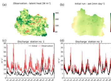
Figure 2.Reference data used for the optimization: the average cloud-free spatial pattern of midday latent heat in June(a)and observed discharge (red line) at two stations (shown in Fig. 1) for the 8-year simulation period(c, d). Also shown are the simulation results from the initial parameter set: the average cloud-free spatial pattern of daily actual evapotranspiration (aet) in June(b)and the simulated discharge (black line) at the two reference stations.

(Fig. 1). Second, in order to complement the temporal data we provide a remote sensing estimate of latent heat for cloud-free grids in June between 2001 and 2008. The month of June is the peak of the growing season, which makes the spatial pattern distinct and relevant for a hydrological model evalu-ation. This reference spatial pattern is obtained by the two-source energy balance model (TSEB; Norman et al., 1995). A detailed description of the remote-sensing-based estimation of latent heat across Denmark is presented by Mendiguren et al. (2017). As outlined by Mendiguren et al. (2017), TSEB represents a two-layer model which separates soil and veg-etation. Energy fluxes are estimated based on various input parameters and forcings among which land surface temper-ature (LST) and air tempertemper-ature are found to be most sen-sitive. Input data for TSEB are obtained from the daytime LST MODIS product at 1 km spatial resolution. The reason-ing behind averagreason-ing the latent heat maps in time to a mean monthly map is expressed twofold. First, daily spatial pat-terns are influenced by clouds and thus vary highly in cov-erage, which limits the pattern information content. Second, daily estimates are associated with higher uncertainty and are more affected by forcing data, e.g. the spatial distribution of precipitation on the previous day. Hence, aggregated monthly maps of latent heat represent a robust average that is more in-formative in a model calibration than daily maps because it constitutes the imprint of soil properties and vegetation on

the simulated pattern, which are parameters that can be cali-brated in a hydrological model in contrast to model forcing. 2.4 Spatial performance metrics

2.4.1 Spatial efficiency

For the formulation of a straightforward spatial performance metric we found inspiration in the Kling–Gupta efficiency (KGE; Kling and Gupta, 2009), which is a commonly used metric in hydrological modelling to evaluate discharge simu-lations. It is characterized by three equally weighted compo-nents, i.e. correlation, variability and bias.

KGE=1− q

αQ−1 2

+ βQ−1 2

+ γQ−1 2

(1) αQ=ρ (obs,sim) , βQ=σsimσobsandγQ=

µsim µobs

whereαQis the Pearson correlation coefficient between the observed (obs) and the simulated (sim) discharge time series, βQ is the relative variability based on the ratio of standard deviation in simulated and observed values and γQ is the bias term which is normalized by the standard deviation of the observed data. KGE is selected as the discharge objective function for the optimization applied in this study.

more holistic and balanced assessment using several aspects is favourable for a comprehensive model evaluation as advo-cated by Gupta et al. (2012), Krause et al. (2005) and others. Following the multiple-component idea of KGE we present a novel spatial performance metric denoted SPA-tial EFficiency (SPAEF), which was originally proposed by Demirel et al. (2018a, b).

SPAEF=1− q

(α−1)2+(β−1)2+(γ−1)2 (2)

α=ρ (obs,sim),β=σsim

µsim

/σobs

µobs

andγ=

n

P

j=1

min(Kj,Lj) n

P

j=1

Kj

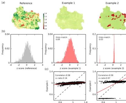
where αis the Pearson correlation coefficient between the observed (obs) and simulated (sim) pattern,βis the fraction of the coefficient of variation representing spatial variability andγis the histogram intersection for the given histogramK of the observed pattern and the histogramLof the simulated pattern, each containing n bins (Swain and Ballard, 1991). In order to enable the comparison of two variables with dif-ferent units and to ensure bias insensitivity, the zscore of the patterns is used to computeγ. Throughout the paperαis referred to as correlation,βas cv ratio andγ as histo match. The difficulty to quantitatively compare spatial patterns and the need for multiple-component metrics such as SPAEF are illustrated in Fig. 3 in which two example patterns both generated by mHM during calibration are compared with the TSEB reference pattern. A swift visual comparison clearly disambiguates the fact that both are inadequate spatial pat-tern representations with respect to the reference; i.e. the first lacks spatial variability and the second misses spatial detail within the clearly separated clusters of high and low values. Correlation is a commonly known statistical measure that allows for the comparison of two variables that are col-located in space and may differ in units. Despite the visual evaluation, both examples have a reasonably high correla-tion, which allegedly suggests good performance. When as-sessing the cv ratio it becomes clear that the first example lacks spatial variability, whereas the distinct separation of the second example suggests an adequate representation of spatial variability. The deficiency of the second example be-comes clear when investigating the overlap of histograms of the normalized (zscore) simulated and reference pattern. The zscore normalization results in a pattern with a mean equal to 0 and a standard deviation equal to 1, which is necessary to make two patterns with different units comparable. Histo match stresses non-existing spatial variability within the high and low areas despite the satisfying correlation and spatial variability.

2.4.2 Connectivity

The connectivity metric originates from the field of hydro-geology in which it is commonly applied to characterize the spatial heterogeneity of aquifers (Koch et al., 2014; Rongier

et al., 2016). Outside the hydrogeology community, connec-tivity analyses have also been conducted to describe the spa-tial patterns of soil moisture (Grayson et al., 2002; Western et al., 2001) and land surface temperature (Koch et al., 2016b). Following the classification of Renard and Allard (2013), the connectivity analysis of a continuous variable is conducted via three steps: (1) a series of threshold percentiles decom-poses the domain into a series of binary maps, (2) the binary maps undergo a cluster analysis that identifies spatially con-nected clusters and (3) the transition from many disconcon-nected clusters to a single connected cluster can be quantified by principles of percolation theory (Hovadik and Larue, 2007). In this context the probability of connection (0) is consid-ered a suitable percolation metric.0states the proportion of pairs of cells that are connected among all possible pairs of connected cells of a cluster map.

0 (t )= 1

n2_t N (Xt)

X

i=1

n2_i, (3)

wherent is the total number of cells in the binary map Xt below or above thresholdt, which hasN (Xt) distinct clus-ters in total.niis the number of cells in theith cluster inXt. The percolation is well captured by means of an increasing threshold that moves along all percentiles of the variable’s range, which makes this methodology bias insensitive. The connectivity analysis is applied individually on cells that ex-ceed a given threshold and those that fall below, which is referred to as the low and high phase, respectively. Follow-ing Koch et al. (2016b), the root mean square error between the connectivity at all percentiles of the observed (0(t )obs) and the simulated (0(t )sim) pattern denotes a tangible pattern similarity metric and can be calculated as

RMSECon= s

P100

t=1(0(t )obs−0(t )sim) 2

100 . (4)

The average RMSE score of the low and the high phase is employed as the pattern similarity score for the connectiv-ity analysis and is referred to as connectivconnectiv-ity throughout the paper.

2.4.3 Fractions skill score

1878 J. Koch et al.: The SPAtial EFficiency metric (SPAEF)

Figure 3.Two examples to illustrate the importance of a multi-component analysis when comparing spatial patterns(a). The maps are normalized by their mean. The histograms of thezscore normalized maps are presented in(b). The scatter plots of the mean normalized maps are given in(c). Scores for the three SPAEF components (histo match, cv ratio and correlation) are given in the graphs.

the simulated (sim) spatial pattern into binary maps. (2) For each cell, compute the fraction of cells that exceed the thresh-old and lie within a window of size n×n and (3) calcu-late the mean squared error (MSE) between the observed and simulated fractions and normalize it with a worst case MSE (MSEwc) that reflects the condition with zero agree-ment between the spatial patterns. The MSE is based on all cells (Nxy) that lie within the modelling domain with dimen-sions ofNxandNy. For a certain threshold, FSS at scalenis given by

FSS(n)=1−

MSE(n) MSE(n)wc

, (5)

where MSE(n)= 1

Nxy Nx

X

i=1 Ny

X

j=1

ref(n)ij−scen(n)ij2 (6) and

MSE(n)wc= 1 Nxy



 Nx

X

i=1 Ny

X

j=1

ref2_(n)ij+

Nx

X

i=1 Ny

X

j=1

scen2_(n)ij 

. (7)

FSS ranges from 0 to 1, where 1 indicates a perfect match between obs and sim and 0 reflects the worst possible perfor-mance. For the simulated spatial patterns in the Skjern catch-ment we applied the concept of critical scales (Koch et al., 2017) and therefore selected three top and three bottom per-centiles each assessed at an individual critical scale. The 1st, 5th and 20th percentiles focus on the bottom 1, 5 and 20 % of cells and are investigated at 25, 15 and 5 km scale, re-spectively. Three top percentiles, the 99th, 95th and 80th, are analysed analogously. The average of the three top and bot-tom percentiles is calculated as an overall pattern similarity score and referred to as FSS throughout the paper.

2.5 Optimization procedure

pattern of June under cloud-free conditions. The reference pattern reflects an instantaneous observation of midday la-tent heat (W m−2_{), whereas the model simulates daily} ac-tual evapotranspiration (mm day−1). Obviously these vari-ables are closely related; however, it requires suitable spatial performance metrics to be able to quantitatively compare two patterns with different units.

A sensitivity analysis was performed in order to select a limited number of parameters for the optimization. This was based on two steps: a variance-based sequential screening (Cuntz et al., 2015) followed by a Latin hypercube sampling (van Griensven et al., 2006). The mHM has 48 global pa-rameters and the first step identified 24 informative parame-ters; results were presented by Demirel et al. (2018a). Subse-quently we applied the Latin hypercube sampling to further reduce the number of sensitive parameters to 17. Among the selected parameters, eight represent the soil moisture mod-ule (pedo transfer functions, root fraction distribution and soil moisture stress), two control the interflow, one affects the percolation, two are sensitive to the base flow and four define the ET module via the dynamic scaling function using MODIS LAI.

In order to reflect on the ability of different spatial per-formance metrics to optimize the pattern perper-formance of the distributed hydrological model applied in this study, we have designed six calibrations. All commence with the same ini-tial parameter set and include KGE at both discharge stations as temporal objective functions. Additionally, each optimiza-tion features one of the promoted spatial performance met-rics: (1) SPAEF, (2) correlation, (3) cv ratio, (4) histo match, (5) FSS and (6) connectivity. The metrics correlation, cv ra-tio and histo match represent the three SPAEF components. The spatial objective functions aim to optimize the average ET pattern of June and are weighted 5 times higher than the discharge objective functions. We expect the capability of the model to optimize simulated time series of discharge to be more versatile in comparison to its flexibility to optimize spatial patterns, which justifies the weighting of the objective functions. The optimizations were conducted with the help of PEST (version 14.02; Doherty, 2005) and the shuffled com-plex evolution (SCE-UA) algorithm (Duan et al., 1993) was selected as an optimizer. SCE-UA is considered a global op-timizer and for our application it was set up to operate on two parallel complexes with 35 parameter sets in each complex. Each calibration was limited to 2500 model runs, which was found reasonable to allow for the convergence of the objec-tive functions.

3 Results and discussion 3.1 Optimizing spatial patterns

The simulation results from the initial parameter set are de-picted in Fig. 2. The simulated pattern of AET is almost

uni-form with very little spatial variability, which results in a low SPAEF score of−0.58. The simulated discharge has the cor-rect timing at both stations: station no. 2 is clearly less biased than station no. 1. Both have reasonable KGE scores on the basis of the initial parameter set: 0.6 (station no. 1) and 0.7 (station no. 2).

Figure 4 visualizes the results from the six conducted cal-ibrations with the aim of tracking the spatial patterns of sim-ulated ET during the course of the optimization. SCE-UA is executed in an iterative manner whereby each iteration reflects a shuffling loop in which a number of parameter sets are tested. In order to inter-compare the optimization progress across the six calibrations, Fig. 4 illustrates the op-timal spatial patterns at four selected iterations during the calibration. The second iteration is the first in which SCE-UA receives feedback from the applied metric after executing random sets of parameter values in the first iteration. Itera-tions 6 and 10 show intermediate steps from the optimization progress. The optimal spatial pattern depicts the final result in accordance with the six tested performance metrics after 2500 model runs.

From a metric point of view, the scores of the objective functions are improved for all six calibrations. Among the six metrics, connectivity is the only one which has to be re-duced to 0; the remaining metrics have an optimal score of 1. The improvements from iteration 10 to the optimal parameter set are numerically marginal and visually not to be discrim-inated. The visual differences between the optimized spatial patterns are striking and the three metrics that consider lo-cal constraints (SPAEF, correlation and FSS) can clearly be distinguished from the remaining three. With respect to the reference pattern in Fig. 2, the separation between forest and non-forest has been inverted by optimizing against cv ratio and connectivity because the right allocation is not reflected by the metrics. The histo match metric is based onzscore normalization, which results in a clear underestimation of spatial variability.

The importance of human-perception-based model evalu-ation has been widely recognized in the literature (Grayson et al., 2002; Hagen, 2003; Koch et al., 2015; Kuhnert et al., 2005). Following our visual evaluation we regard the SPAEF optimization as the most similar to the reference in Fig. 2. The three SPAEF components lead to very diverging solu-tions, and combined as SPAEF, the optimization yields a spa-tial pattern which adequately reflects the imprint of both veg-etation and soil on the simulated ET patterns. FSS as an ob-jective function performs almost equally satisfying, and re-visiting the defined critical scales may improve this calibra-tion result even further.

cer-1880 J. Koch et al.: The SPAtial EFficiency metric (SPAEF)

Figure 4.Tracking of the simulated actual evapotranspiration maps (normalized by mean) throughout the six conducted optimizations using different objective functions. The first four columns show the trajectory of pattern improvements in accordance with one objective function. The maps depict the best fit between the reference(b)and model at various iterations throughout the optimization. The spatial similarity scores in accordance with the different metrics are given in the top right corner of each map.

tain extent. In consequence, these metrics do not function as stand-alone objective functions for this calibration study; e.g. cv ratio yields an inadequate spatial pattern but as a com-ponent in SPAEF it generates a satisfying solution to the optimization problem. Following Krause et al. (2005), one should carefully take the pros and cons of each performance measure into consideration when designing the calibration and validation framework of a model. Moreover, the met-ric should be tailored to the intended use of the model and should relate to simulated quantities which are deemed rele-vant for the application of the model. For the objective of our calibration study the bias insensitivity and the capability of a metric to compare variables that are related but differ in unit was most relevant.

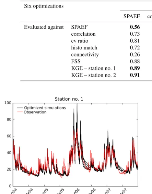
Table 1 cross-checks the metric scores of the six optimized spatial patterns in Fig. 4. Reading the table column-wise al-lows for an investigation of whether the metrics provide in-dependent information to the optimizer. As an example, cv ratio reaches its optimal score; however, the reaming metrics perform poorly. This indicates that cv ratio conveys indepen-dent information with respect to the other metrics. On the other hand, calibrating against correlation yields a high FSS score, which attests partly redundant information content in the two given metrics. Reading the table row-wise screens for the consistency of the calibrations. The highest metric score

should be reached when calibrating against itself, which is the case for all six calibrations.

Additionally, Table 1 presents the KGE scores for the six conducted calibrations. The discharge performance has been improved by all calibrations and the scores vary slightly across them. Similar to the initial run station no. 2 performs generally better than station no. 1. The simulated discharge of the six optimized models is shown in Fig. 5 for a 4-year period at station no. 1. All calibrations simulate the discharge dynamics in accordance with the observations and are gener-ally equipped with a good timing of the peak flows. Differ-ences are found in the recession flow between the six sim-ulations. However, our effort focuses on the spatial perfor-mance and it is striking how different the simulated spatial patterns can be while predicting almost identical streamflow. This supports previous findings in the literature which stress that spatial and temporal response in hydrological models are controlled by different parameters and that the one cannot be used to inform the other (Pokhrel and Gupta, 2011; Stisen et al., 2011, and others).

cap-Table 1.Cross-check of the six conducted calibrations (as rows). The optimal model run is evaluated by the remaining metrics (as columns). Numbers in bold indicate the optimized value of the respective optimization.

Six optimizations Calibrated against

SPAEF correlation cv ratio histo match connectivity FSS

Evaluated against SPAEF 0.56 0.28 −0.74 −0.19 −1.16 0.18

correlation 0.73 0.80 −0.48 0.15 −0.56 0.74

cv ratio 0.81 0.41 1.00 0.17 2.17 0.57

histo match 0.72 0.64 0.10 0.91 0.08 0.36

connectivity 0.26 0.18 0.17 0.25 0.10 0.18

FSS 0.88 0.91 0.44 0.35 0.40 0.91

KGE – station no. 1 0.89 0.90 0.88 0.84 0.88 0.95

KGE – station no. 2 0.91 0.93 0.91 0.90 0.92 0.95

Figure 5.Simulated discharge at station no. 1 obtained by the six optimizations. Data are shown only for 4 out of the 8 years of sim-ulation. KGE values vary between 0.84 and 0.95.

ture the correct spatial allocation, variability and distribution. Thus, the key weakness of connectivity is that it cannot op-erate as a stand-alone metric; instead it should be accompa-nied by another metric, ideally correlation, which will ensure the correct allocation. On the other hand, FSS yields reason-able scores of allocation and variability between forest and non-forest areas. However, the FSS optimization lacks spa-tial variability within the high and low areas, which could be resolved by considering more threshold percentiles when computing the score. Therefore the weakness of FSS lies in its dependency on the threshold percentile, which has to be defined by the user.

Choosing a suitable metric alone is not sufficient to un-dertake a successful spatial-pattern-oriented model calibra-tion. Model agility promoted by a flexible parameterization is required to allow the simulated spatial patterns to be op-timized with respect to a reference pattern (Mendoza et al., 2015). In this study, this is achieved by applying a model code (mHM: Samaniego et al., 2010a) that features a multi-scale parameter regionalization scheme (MPR) in which

spa-tially distributed basin characteristics are transformed via global parameters to effective model parameters at the model scale. These so-called transfer functions generate seamless and physically consistent parameters fields (Mizukami et al., 2017). In contrast, Corbari and Mancini (2014) conducted a spatial validation of a subsurface–surface–land surface model against MODIS LST in which parameters were cali-brated individually at each grid. In contrast to regionalization techniques such as MPR, this approach does not grant phys-ically meaningful parameter fields and may overestimate the credibility of remote sensing data. Samaniego et al. (2017b) recently proposed a modelling protocol that describes how MPR can be added to any particular model, which extends the applicability of MPR beyond mHM. However, the choice of transfer functions may not always be trivial and their re-liability is crucial for the successful application of MPR or other regionalization approaches. Another limitation of the MPR scheme in mHM is that the minimum scale at which a model can be applied depends on the data availability, since subgrid variability is fundamental to MPR (Samaniego et al., 2017b).

In order to examine the added value of spatial patterns retrieved from remote sensing data, Demirel et al. (2018a) conducted several calibration scenarios of the same model set-up as applied in this study. Calibrating only against time series of discharge resulted in a poor spatial pattern perfor-mance and, vice versa, the calibration using remote sensing data only was not able to constrain the hydrograph correctly. However, the balanced calibration using both observations did not worsen the objective function in comparison to using them as the sole calibration target, which underlined limited trade-offs between the temporal and spatial observations in the applied calibration.

1882 J. Koch et al.: The SPAtial EFficiency metric (SPAEF)

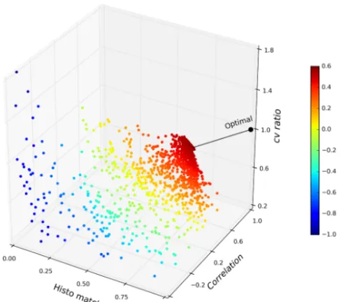
Figure 6.3-D Pareto front based on the 2500 runs during the SPAEF optimization. Each component of the SPAEF metric represents an individual axis. The black line indicates the deviation between the theoretical optimal (1,1,1) SPAEF value and the optimized model run (0.72,0.73,0.81).

evaluation against SMAP brightness temperature. Similar so-lutions are feasible for LST and it has the clear advantage of bypassing the uncertainties and inconsistencies associated with remote sensing models, which the hydrological mod-eller has no control of.

3.2 Spatial efficiency metric

Establishing novel metrics in the modelling community is of-ten hindered by an intrinsic inertia supported by an excessive choice of metrics, which leads to reliance on familiar metrics. Both the implementation and the interpretation of unfamiliar metrics may be found too troublesome by many users. Famil-iarity can only be obtained by rigorous testing and by having a metric which provides scores in a predefined range easy to interpret. In the following we will provide a detailed analysis of the SPAEF calibration results to further the understand-ing of its implications and the interaction between the three components.

Figure 6 depicts a three-dimensional Pareto front of the three SPAEF components on the basis of the 2500 parameter sets executed in the SPAEF calibration, which allows for an investigation of trade-offs between different objective func-tions. The formulation of SPAEF gives equal weights to the three components; hence the best compromise is the parame-ter set with the lowest Euclidian distance to the optimal point (1,1,1). If desirable, the weights could be adjusted manu-ally to specificmanu-ally focus on one of the three components. Throughout calibration, scores across the range of each

com-ponent are obtained, which indicates that the comcom-ponents are clearly sensitive to changes in spatial performance. Further, it reveals the global nature of SCE-UA, which rigorously ex-plores the parameter space. With an ideal score of 1, SCE-UA optimized SPAEF to 0.56, which may seem surprisingly low given the good visual agreement. This underlines the fact that SPAEF is a tough criterion with three independent components that individually penalize the overall similarity score. The question of what marks an acceptable and satisfy-ing SPAEF score is hard to generalize and probably depends on the pattern to be assessed. The ET pattern in the Skjern catchment is dominated by local feedbacks of soil and vege-tation, which constitute challenging small-scale details for a model. Alternatively, a catchment with a strong spatial gra-dient of e.g. precipitation or topography may naturally yield a higher SPAEF score. Such gradients in forcing or morphol-ogy are typically not calibrated and will dominate the spatial pattern of the estimated hydrological fluxes. A distinct spa-tial variability provided by the model inputs is therefore ex-pected to favour correlation and cv ratio, resulting in a higher SPAEF score. However, more work is needed to study the re-lationship of spatial variability and SPAEF.

The patterns of the simulated variable (daily ET) and the observed variable (instantaneous latent heat) used in this study differ in unit but are linearly related. One can imagine a case of using SPAEF in a proxy validation with a non-linear relationship between the variables. In such a case, the user can consider transforming the data. This is especially cru-cial for correlation, which assumes linearity. The remaining components, histo match and cv ratio, are less dependent on linearity, as the first is based onzscore normalization and the second on mean normalization.

As introduced earlier, human perception is considered a reliable benchmark for the evaluation of spatial performance metrics. More precisely, a metric can be regarded as reliable if it is able to emulate human vision. In order to establish a re-liable benchmark dataset, Koch and Stisen (2017) have con-ducted a citizen science project with the aim of quantifying spatial similarity scores based on human perception. Their study was based on over 6000 simulated spatial pattern com-parisons of land surface variables in the Skjern catchment. When compared to human perception, SPAEF provides a sat-isfying coefficient of determination of 0.73. In comparison, the coefficients of determination for connectivity, FSS and correlation are 0.48, 0.60 and 0.76, respectively.

Figure 7.Tracking of the three SPAEF components throughout the 2500 conducted runs of four calibrations (SPAEF, correlation, cv ratio and histo match). The envelopes represent the 10th and 90th percentile of a 100-run moving window; the line shows the median.

be considered independent because optimizing against one component does not automatically lead to the improvement of another. This is especially the case for the cv ratio calibra-tion in which correlacalibra-tion stagnates and histo match decreases throughout the course of the 2500 runs.

Uncertainty in the observations should ideally be an in-tegral part of model evaluation. The proposed calibration framework in this study deals implicitly with the issue of uncertainty. First, the daily snapshots of midday ET are av-eraged to a more robust monthly map, and second, the bias insensitivity of SPAEF alleviates the effect of uncertainties in the observations. Instead of assessing the exact values at the grid scale, SPAEF evaluates global characteristics such as distribution and variability, which are less affected by data uncertainty. For some applications, the bias insensitivity may be a hurdle when the model is expected to be unbiased. In such a case the SPAEF formulation (Eq. 4) could easily be extended by a fourth component, such as the bias term (γQ) from the KGE formulation (Eq. 3). Discharge obser-vations are most commonly available for hydrological mod-elling studies. Such data can provide reliable information on the overall water balance, and when being accompanied with spatial observations, the catchment internal variability of hy-drological processes can be constrained as well.

4 Conclusions

The complexity of spatially distributed hydrological models is currently increasing, as is the availability of satellite-based

remote sensing observations. In light of the vast amount of existing remote sensing products in combination with re-cent developments, such as the promising Copernicus pro-gramme with its multi-satellite Sentinel missions (McCabe et al., 2017), the incorporation of detailed spatial data retrieved from remote sensing platforms will continue to enable grand opportunities for hydrological modelling in the near future.

This study aimed to make a contribution to that course by rigorously testing SPAEF, a simple and novel spatial perfor-mance metric which has the potential to advance the spatial-pattern-oriented validation and calibration of spatially dis-tributed models. The applicability of SPAEF was tested in the hydrological context; however, its versatility promotes it to be beneficial throughout many disciplines of earth system modelling.

We applied SPAEF alongside its three components and two other spatial performance metrics (connectivity and FSS) in a calibration experiment of a mesoscale catchment (∼2500 km2) in Denmark. A satellite-retrieved map of latent heat, which represents the average evapotranspiration pattern of cloud-free days in June, was utilized beside discharge time series as the reference dataset. We draw the following main conclusions from this work.

Quantifying spatial similarity is a non-trivial task and it requires taking several dimensions of spatial information si-multaneously into consideration. The formulation of SPAEF is therefore based on three equally weighted components, i.e. correlation, ratio of the coefficient of variation andzscore histogram overlap between a simulated and an observed pat-tern. SPAEF reflects the Euclidian distance of the three com-ponents from the optimum, which is equivalent to the con-cept of a three-dimensional Pareto front. The components are bias insensitive and allow for the assessment of two variables that differ in units. Further, we could infer independent infor-mation content on the three components, which complement each other when used jointly as SPAEF.

SPAEF is straightforward to compute and has a predefined range between−∞and 1, which simplifies communication with the scientific community and stakeholders. Neverthe-less, more rigorous testing is required to further establish fa-miliarity. The relationship between SPAEF and spatial vari-ability has to be investigated in more detail for the purpose of putting the metric into context, i.e. comparing different catchments or models.

The right spatial performance metric alone is not enough to improve the spatial predictability of a distributed model trough calibration. The metric has to be accompanied by an agile model structure and flexible parameterization, such as regionalization techniques, by means of transfer functions, allowing the simulated pattern to adjust in a meaningful way. Naturally, this has to be further supported by high-quality forcing data, detailed catchment morphology and trustworthy spatial observations at an adequate scale.

1884 J. Koch et al.: The SPAtial EFficiency metric (SPAEF)

in the calibration of hydrological models since the six con-ducted calibrations yielded strikingly different ET patterns while simulating similar discharge dynamics. Based on our findings, bias insensitive spatial metrics are ideally accompa-nied by bias sensitive discharge metrics that secure the over-all robustness in terms water balance closure.

With this contribution we hope to encourage the modelling community to rethink paradigms when formulating calibra-tion or validacalibra-tion experiments by choosing appropriate met-rics that focus on spatial patterns representing earth system processes.

Code and data availability. The code for the applied spatial perfor-mance metrics is made available by Demirel et al. (2018b) at https: //github.com/cuneyd/spaef and Koch (2018) at https://github.com/ JulKoch/SEEM. The mHM code is freely accessible via GitHub at https://github.com/mhm-ufz/mhm (Samaniego et al., 2017a). All data used to produce the results of this paper will be provided upon request by contacting Julian Koch.

Competing interests. The authors declare that they have no conflict of interest.

Acknowledgements. The scientific work has been carried out under the SPACE (SPAtial Calibration and Evaluation in distributed hydrological modelling using satellite remote sensing data) project (grant VKR023443), which is funded by the Villum Foundation.

Edited by: Tomomichi Kato

Reviewed by: Naoki Mizukami and one anonymous referee

References

Alexandrov, G. A., Ames, D., Bellocchi, G., Bruen, M., Crout, N., Erechtchoukova, M., Hildebrandt, A., Hoffman, F., Jack-isch, C., Khaiter, P., Mannina, G., Matsunaga, T., Purucker, S. T., Rivington, M., and Samaniego, L.: Technical assess-ment and evaluation of environassess-mental models and software: Letter to the Editor, Environ. Model. Softw., 26, 328–336, https://doi.org/10.1016/j.envsoft.2010.08.004, 2011.

Bennett, N. D., Croke, B. F. W., Guariso, G., Guillaume, J. H. A., Hamilton, S. H., Jakeman, A. J., Marsili-Libelli, S., Newham, L. T. H., Norton, J. P., Perrin, C., Pierce, S. A., Robson, B., Sep-pelt, R., Voinov, A. A., Fath, B. D., and Andreassian, V.: Charac-terising performance of environmental models, Environ. Model. Softw., 40, 1–20, https://doi.org/10.1016/j.envsoft.2012.09.011, 2013.

Brown, B. G., Gotway, J. H., Bullock, R., Gilleland, E., Fowler, T., Ahijevych, D., and Jensen, T.: The Model Evaluation Tools (MET): Community tools for forecast evaluation, in: Preprints, 25th Conf. on International Interactive Information and Process-ing Systems (IIPS) for Meteorology, Oceanography, and Hydrol-ogy, Phoenix, AZ, Amer. Meteor. Soc. A, Vol. 9, 2009.

Clark, M. P., Kavetski, D., and Fenicia, F.: Pursuing the method of multiple working hypotheses for hydro-logical modeling, Water Resour. Res., 47, W09301, https://doi.org/10.1029/2010WR009827, 2011.

Cloke, H. L. and Pappenberger, F.: Evaluating forecasts of extreme events for hydrological applications: An approach for screening unfamiliar performance measures, Meteorol. Appl., 15, 181–197, 2008.

Corbari, C. and Mancini, M.: Calibration and Validation of a Distributed Energy–Water Balance Model Using Satel-lite Data of Land Surface Temperature and Ground Dis-charge Measurements, J. Hydrometeorol., 15, 376–392, https://doi.org/10.1175/JHM-D-12-0173.1, 2014.

Cuntz, M., Mai, J., Zink, M., Thober, S., Kumar, R., Schäfer, D., Schrön, M., Craven, J., Rakovec, O., Spieler, D., Prykhodko, V., Dalmasso, G., Musuuza, J., Langenberg, B., Attinger, S., and Samaniego, L.: Computationally inexpen-sive identification of noninformative model parameters by sequential screening, Water Resour. Res., 51, 6417–6441, https://doi.org/10.1002/2015WR016907, 2015.

Dawson, C. W., Abrahart, R. J., and See, L. M.: HydroTest: A web-based toolbox of evaluation metrics for the standardised as-sessment of hydrological forecasts, Environ. Modell. Softw., 22, 1034–1052, https://doi.org/10.1016/j.envsoft.2006.06.008, 2007. Demirel, M. C., Mai, J., Mendiguren, G., Koch, J., Samaniego, L., and Stisen, S.: Combining satellite data and appropriate objec-tive functions for improved spatial pattern performance of a dis-tributed hydrologic model, Hydrol. Earth Syst. Sci., 22, 1299– 1315, https://doi.org/10.5194/hess-22-1299-2018, 2018a. Demirel, M. C., Stisen, S., and Koch, J.: SPAEF: SPAtial

EFfi-ciency, https://doi.org/10.5281/ZENODO.1158890, 2018b. Doherty, J.: PEST: Model Independent Parameter Estimation. Fifth

Edition of User Manual, Watermark Numerical Computing, Bris-bane, 2005.

Dorninger, M., Mittermaier, M. P., Gilleland, E., Ebert, E. E., Brown, B. G., and Wilson, L. J.: MesoVICT: Mesoscale Verification Inter-Comparison over Complex Terrain. NCAR Technical Note NCAR/TN-505+STR, 23 pp., https://doi.org/10.5065/D6416V21, 2013.

Duan, Q. Y., Gupta, V. K., and Sorooshian, S.: Shuffled com-plex evolution approach for effective and efficient global minimization, J. Optimiz. Theory App., 76, 501–521, https://doi.org/10.1007/BF00939380, 1993.

Gilleland, E., Ahijevych, D., Brown, B. G., Casati, B., and Ebert, E. E.: Intercomparison of Spatial Forecast Verification Methods, Weather Forecast., 24, 1416–1430, 2009.

Gilleland, E., Bukovsky, M., Williams, C. L., McGinnis, S., Am-mann, C. M., Brown, B. G., and Mearns, L. O.: Evaluating NAR-CCAP model performance for frequencies of severe-storm en-vironments, Adv. Stat. Clim. Meteorol. Oceanogr., 2, 137–153, https://doi.org/10.5194/ascmo-2-137-2016, 2016.

Glaser, B., Klaus, J., Frei, S., Frentress, J., Pfister, L., and Hopp, L.: On the value of surface saturated area dynamics mapped with thermal infrared imagery for modeling the hillslope-riparian-stream continuum, Water Resour. Res., 52, 8317–8342, https://doi.org/10.1002/2015WR018414, 2016.

Grayson, R. B., Blöschl, G., Western, A. W., and McMahon, T. A.: Advances in the use of observed spatial patterns of catch-ment hydrological response, Adv. Water Resour., 25, 1313–1334, https://doi.org/10.1016/s0309-1708(02)00060-x, 2002.

Gupta, H. V., Wagener, T., and Liu, Y. Q.: Reconciling theory with observations: elements of a diagnostic ap-proach to model evaluation, Hydrol. Process., 22, 3802–3813, https://doi.org/10.1002/Hyp.6989, 2008.

Gupta, H. V., Clark, M. P., Vrugt, J. A., Abramowitz, G., and Ye, M.: Towards a comprehensive assessment of model structural adequacy, Water Resour. Res., 48, W08301, https://doi.org/10.1029/2011WR011044, 2012.

Hagen, A.: Fuzzy set approach to assessing similarity of categorical maps, Int. J. Geogr. Inf. Sci., 17, 235–249, https://doi.org/10.1080/13658810210157822, 2003.

Hagen, A. and Martens, P.: Map comparison methods for com-prehensive assessment of geosimulation models, International Conference on Computational Science and Its Applications, Springer, Berlin, Heidelberg, 2008.

Herrera-Estrada, J. E., Satoh, Y., and Sheffield, J.: Spatiotemporal dynamics of global drought, Geophys. Res. Lett., 44, 2254–2263, https://doi.org/10.1002/2016GL071768, 2017.

Hovadik, J. M. and Larue, D. K.: Static characterizations of reser-voirs: refining the concepts of connectivity and continuity, Petrol. Geosci., 13, 195–211, 2007.

Immerzeel, W. W. and Droogers, P.: Calibration of a distributed hydrological model based on satel-lite evapotranspiration, J. Hydrol., 349, 411–424, https://doi.org/10.1016/j.jhydrol.2007.11.017, 2008.

Jensen, K. H. and Illangasekare, T. H.: HOBE: A Hy-drological Observatory, Vadose Zone J., 10, 1–7, https://doi.org/10.2136/vzj2011.0006, 2011.

Kling, H. and Gupta, H.: On the development of regionalization relationships for lumped watershed models: The impact of ig-noring sub-basin scale variability, J. Hydrol., 373, 337–351, https://doi.org/10.1016/j.jhydrol.2009.04.031, 2009.

Kling, H., Fuchs, M., and Paulin, M.: Runoff conditions in the upper Danube basin under an ensemble of cli-mate change scenarios, J. Hydrol., 424–425, 264–277, https://doi.org/10.1016/J.JHYDROL.2012.01.011, 2012. Koch, J.: SEEM: Spatial Evaluation of Environmental Models,

https://doi.org/10.5281/zenodo.1154614, 2018.

Koch, J. and Stisen, S.: Citizen science: A new perspective to ad-vance spatial pattern evaluation in hydrology, PLoS One, 12, 1– 20, https://doi.org/10.1371/journal.pone.0178165, 2017. Koch, J., He, X., Jensen, K. H., and Refsgaard, J. C.: Challenges

in conditioning a stochastic geological model of a heterogeneous glacial aquifer to a comprehensive soft data set, Hydrol. Earth Syst. Sci., 18, 2907–2923, https://doi.org/10.5194/hess-18-2907-2014, 2014.

Koch, J., Jensen, K. H., and Stisen, S.: Toward a true spa-tial model evaluation in distributed hydrological modeling: Kappa statistics, Fuzzy theory, and EOF-analysis bench-marked by the human perception and evaluated against a modeling case study, Water Resour. Res., 51, 1225–1246, https://doi.org/10.1002/2014WR016607, 2015.

Koch, J., Cornelissen, T., Fang, Z., Bogena, H., Diekkrüger, B., Kollet, S., and Stisen, S.: Inter-comparison of three distributed hydrological models with respect to seasonal variability of soil

moisture patterns at a small forested catchment, J. Hydrol., 533, 234–249, https://doi.org/10.1016/j.jhydrol.2015.12.002, 2016a. Koch, J., Siemann, A., Stisen, S., and Sheffield, J.: Spatial

val-idation of large scale land surface models against monthly land surface temperature patterns using innovative perfor-mance metrics, J. Geophys. Res.-Atmos., 121, 5430–5452, https://doi.org/10.1002/2015JD024482, 2016b.

Koch, J., Mendiguren, G., Mariethoz, G., and Stisen, S.: Spa-tial sensitivity analysis of simulated land-surface patterns in a catchment model using a set of innovative spatial performance metrics, J. Hydrometeorol., 18, 1121–1142, JHM-D-16-0148.1, https://doi.org/10.1175/JHM-D-16-0148.1, 2017.

Krause, P., Boyle, D. P., and Bäse, F.: Comparison of different effi-ciency criteria for hydrological model assessment, Adv. Geosci., 5, 89–97, https://doi.org/10.5194/adgeo-5-89-2005, 2005. Kuhnert, M., Voinov, A., and Seppelt, R.: Comparing raster map

comparison algorithms for spatial modeling and analysis, Pho-togramm. Eng. Remote Sensing, 71, 975–984, 2005.

Kumar, R., Samaniego, L., and Attinger, S.: The effects of spa-tial discretization and model parameterization on the predic-tion of extreme runoff characteristics, J. Hydrol., 392, 54–69, https://doi.org/10.1016/j.jhydrol.2010.07.047, 2010.

Kumar, R., Samaniego, L., and Attinger, S.: Implications of dis-tributed hydrologic model parameterization on water fluxes at multiple scales and locations, Water Resour. Res., 49, 360–379, https://doi.org/10.1029/2012WR012195, 2013.

Kumar, S. V., Peters-Lidard, C. D., Santanello, J., Harrison, K., Liu, Y., and Shaw, M.: Land surface Verification Toolkit (LVT) – a generalized framework for land surface model evaluation, Geosci. Model Dev., 5, 869–886, https://doi.org/10.5194/gmd-5-869-2012, 2012.

McCabe, M. F., Wood, E. F., Wjcik, R., Pan, M., Sheffield, J., Gao, H., and Su, H.: Hydrological consistency us-ing multi-sensor remote sensus-ing data for water and en-ergy cycle studies, Remote Sens. Environ., 112, 430–444, https://doi.org/10.1016/j.rse.2007.03.027, 2008.

McCabe, M. F., Rodell, M., Alsdorf, D. E., Miralles, D. G., Uijlen-hoet, R., Wagner, W., Lucieer, A., Houborg, R., Verhoest, N. E. C., Franz, T. E., Shi, J., Gao, H., and Wood, E. F.: The future of Earth observation in hydrology, Hydrol. Earth Syst. Sci., 21, 3879–3914, https://doi.org/10.5194/hess-21-3879-2017, 2017. Mendiguren, G., Koch, J., and Stisen, S.: Spatial pattern evaluation

of a calibrated national hydrological model – a remote-sensing-based diagnostic approach, Hydrol. Earth Syst. Sci., 21, 5987– 6005, https://doi.org/10.5194/hess-21-5987-2017, 2017. Mendoza, P. A., Clark, M. P., Barlage, M., Rajagopalan,

B., Samaniego, L., Abramowitz, G., and Gupta, H.: Are we unnecessarily constraining the agility of complex process-based models?, Water Resour. Res., 51, 716–728, https://doi.org/10.1002/2014WR015820, 2015.

Mittermaier, M., Roberts, N. and Thompson, S. A.: A long-term assessment of precipitation forecast skill using the Fractions Skill Score, Meteorol. Appl., 20, 176–186, https://doi.org/10.1002/met.296, 2013.

1886 J. Koch et al.: The SPAtial EFficiency metric (SPAEF)

Moriasi, D. N., Arnold, J. G., Van Liew, M. W., Bingner, R. L., Harmel, R. D., and Veith, T. L.: Model Eval-uation Guidelines for Systematic Quantification of Accu-racy in Watershed Simulations, T. ASABE, 50, 885–900, https://doi.org/10.13031/2013.23153, 2007.

Norman, J. M., Kustas, W. P., and Humes, K. S.: Source ap-proach for estimating soil and vegetation energy fluxes in ob-servations of directional radiometric surface temperature, Agr. Forest Meteorol., 77, 263–293, https://doi.org/10.1016/0168-1923(95)02265-Y, 1995.

Orth, R., Dutra, E., Trigo, I. F., and Balsamo, G.: Ad-vancing land surface model development with satellite-based Earth observations, Hydrol. Earth Syst. Sci., 21, 2483–2495, https://doi.org/10.5194/hess-21-2483-2017, 2017.

Pokhrel, P. and Gupta, H. V.: On the ability to infer spatial catch-ment variability using streamflow hydrographs, Water Resour. Res., 47, W08534, https://doi.org/10.1029/2010wr009873, 2011. Refsgaard, J. C. and Henriksen, H. J.: Modelling guidelines – Ter-minology and guiding principles, Adv. Water Resour., 27, 71–82, https://doi.org/10.1016/j.advwatres.2003.08.006, 2004. Refsgaard, J. C., Auken, E., Bamberg, C. A., Christensen, B.

S. B., Clausen, T., Dalgaard, E., Effersø, F., Ernstsen, V., Gertz, F., Hansen, A. L., He, X., Jacobsen, B. H., Jensen, K. H., Jørgensen, F., Jørgensen, L. F., Koch, J., Nilsson, B., Petersen, C., De Schepper, G., Schamper, C., Sørensen, K. I., Therrien, R., Thirup, C., and Viezzoli, A.: Nitrate reduc-tion in geologically heterogeneous catchments – A frame-work for assessing the scale of predictive capability of hy-drological models, Sci. Total Environ., 468–469, 1278–1288, https://doi.org/10.1016/j.scitotenv.2013.07.042, 2014.

Renard, P. and Allard, D.: Connectivity metrics for subsur-face flow and transport, Adv. Water Resour., 51, 168–196, https://doi.org/10.1016/j.advwatres.2011.12.001, 2013. Roberts, N.: Assessing the spatial and temporal variation in the skill

of precipitation forecasts from an NWP model, Meteorol. Appl., 15, 163–169, 2008.

Roberts, N. M. and Lean, H. W.: Scale-Selective Verifica-tion of Rainfall AccumulaVerifica-tions from High-ResoluVerifica-tion Fore-casts of Convective Events, Mon. Weather Rev., 136, 78–97, https://doi.org/10.1175/2007MWR2123.1, 2008.

Rongier, G., Collon, P., Renard, P., Straubhaar, J., and Sausse, J.: Comparing connected structures in ensem-ble of random fields, Adv. Water Resour., 96, 145–169, https://doi.org/10.1016/j.advwatres.2016.07.008, 2016. Ruiz-Pérez, G., González-Sanchis, M., Del Campo, A. D., and

Francés, F.: Can a parsimonious model implemented with satel-lite data be used for modelling the vegetation dynamics and wa-ter cycle in wawa-ter-controlled environments?, Ecol. Modell., 324, 45–53, https://doi.org/10.1016/j.ecolmodel.2016.01.002, 2016. Samaniego, L., Kumar, R., and Attinger, S.: Multiscale

pa-rameter regionalization of a grid-based hydrologic model at the mesoscale, Water Resour. Res., 46, W05523, https://doi.org/10.1029/2008wr007327, 2010a.

Samaniego, L., Bardossy, A., and Kumar, R.: Streamflow prediction in ungauged catchments using copula-based dissimilarity measures, Water Resour. Res., 46, W02506, https://doi.org/10.1029/2008WR007695, 2010b.

Samaniego, L., Kumar, R., Mai, J., Zink, M., Thober, S., Cuntz, M., Rakovec, O., Schäfer, D., Schrön, M.,

Bren-ner, J., Demirel, C. M., Kaluza, M., Langenberg, B., Stisen, S., and Attinger, S.: mesoscale Hydrologic Model, https://doi.org/10.5281/ZENODO.1069203, 2017a.

Samaniego, L., Kumar, R., Thober, S., Rakovec, O., Zink, M., Wan-ders, N., Eisner, S., Müller Schmied, H., Sutanudjaja, E. H., Warrach-Sagi, K., and Attinger, S.: Toward seamless hydrologic predictions across spatial scales, Hydrol. Earth Syst. Sci., 21, 4323–4346, https://doi.org/10.5194/hess-21-4323-2017, 2017b. Schaefi, B. and Gupta, H. V.: Do Nash values have value?, Hydrol.

Process., 21, 2075–2080, 2007.

Schalge, B., Rihani, J., Baroni, G., Erdal, D., Geppert, G., Hae-fliger, V., Haese, B., Saavedra, P., Neuweiler, I., Hendricks Franssen, H.-J., Ament, F., Attinger, S., Cirpka, O. A., Kol-let, S., Kunstmann, H., Vereecken, H., and Simmer, C.: High-Resolution Virtual Catchment Simulations of the Subsurface-Land Surface-Atmosphere System, Hydrol. Earth Syst. Sci. Dis-cuss., https://doi.org/10.5194/hess-2016-557, 2016.

Schuurmans, J. M., van Geer, F. C., and Bierkens, M. F. P.: Remotely sensed latent heat fluxes for model error diagno-sis: a case study, Hydrol. Earth Syst. Sci., 15, 759–769, https://doi.org/10.5194/hess-15-759-2011, 2011.

Stisen, S., McCabe, M. F., Refsgaard, J. C., Lerer, S., and Butts, M. B.: Model parameter analysis using remotely sensed pattern in-formation in a multi-constraint framework, J. Hydrol., 409, 337– 349, https://doi.org/10.1016/j.jhydrol.2011.08.030, 2011. Stisen, S., Sonnenborg, T. O., Refsgaard, J. C., Koch, J.,

Bircher, S., and Jensen, K. H.: Moving beyond runoff cali-bration – Multi-constraint optimization of a surface-subsurface-atmosphere model, Hydrol. Process., in revision, 2018. Swain, M. J. and Ballard, D. H.: Color indexing, Int. J. Comput.

Vis., 7, 11–32, https://doi.org/10.1007/BF00130487, 1991. Terink, W., Lutz, A. F., Simons, G. W. H., Immerzeel, W. W.,

and Droogers, P.: SPHY v2.0: Spatial Processes in HYdrology, Geosci. Model Dev., 8, 2009–2034, https://doi.org/10.5194/gmd-8-2009-2015, 2015.

van Griensven, A., Meixner, T., Grunwald, S., Bishop, T., Diluzio, M., and Srinivasan, R.: A global sensitivity analysis tool for the parameters of multi-variable catchment models, J. Hydrol., 324, 10–23, https://doi.org/10.1016/j.jhydrol.2005.09.008, 2006. Vereecken, H., Pachepsky, Y., Simmer, C., Rihani, J., Kunoth, A.,

Korres, W., Graf, A., Franssen, H. J.-H., Thiele-Eich, I., and Shao, Y.: On the role of patterns in understanding the functioning of soil-vegetation-atmosphere systems, J. Hydrol., 542, 63–86, https://doi.org/10.1016/j.jhydrol.2016.08.053, 2016.

Wealands, S. R., Grayson, R. B., and Walker, J. P.: Quantitative comparison of spatial fields for hydrological model assessment – some promising approaches, Adv. Water Resour., 28, 15–32, https://doi.org/10.1016/j.advwatres.2004.10.001, 2005. Western, A. W., Blöschl, G., and Grayson, R. B.: Toward capturing

hydrologically significant connectivity in spatial patterns, Water Resour. Res., 37, 83–97, 2001.