© Author(s) 2017. This work is distributed under the Creative Commons Attribution 3.0 License.
Tiling soil textures for terrestrial ecosystem modelling via clustering
analysis: a case study with CLASS-CTEM (version 2.1)
Joe R. Melton1, Reinel Sospedra-Alfonso2, and Kelly E. McCusker2,3,a
1Climate Research Division, Environment and Climate Change Canada, Victoria, B.C., Canada 2Canadian Centre for Climate Modelling and Analysis, Climate Research Division,
Environment and Climate Change Canada, Victoria, B.C., Canada
3School of Earth and Ocean Sciences, University of Victoria, Victoria, B.C., Canada anow at: Department of Atmospheric Sciences, University of Washington, Seattle, USA
Correspondence to:Joe R. Melton ([email protected]) Received: 9 January 2017 – Discussion started: 3 February 2017
Revised: 7 June 2017 – Accepted: 14 June 2017 – Published: 17 July 2017
Abstract.We investigate the application of clustering algo-rithms to represent sub-grid scale variability in soil texture for use in a global-scale terrestrial ecosystem model. Our model, the coupled Canadian Land Surface Scheme – Cana-dian Terrestrial Ecosystem Model (CLASS-CTEM), is typ-ically implemented at a coarse spatial resolution (approxi-mately 2.8◦×2.8◦) due to its use as the land surface com-ponent of the Canadian Earth System Model (CanESM). CLASS-CTEM can, however, be run with tiling of the land surface as a means to represent sub-grid heterogeneity. We first determined that the model was sensitive to tiling of the soil textures via an idealized test case before attempting to cluster soil textures globally. To cluster a high-resolution soil texture dataset onto our coarse model grid, we use two linked algorithms – the Ordering Points to Identify the Clus-tering Structure (OPTICS) algorithm (Ankerst et al., 1999; Daszykowski et al., 2002) and the algorithm of (Sander et al., 2003) – to provide tiles of representative soil textures for use as CLASS-CTEM inputs. The clustering process results in, on average, about three tiles per CLASS-CTEM grid cell with most cells having four or less tiles. Results from CLASS-CTEM simulations conducted with the tiled inputs (Cluster) versus those using a simple grid-mean soil texture (Gridmean) show CLASS-CTEM, at least on a global scale, is relatively insensitive to the tiled soil textures; however, dif-ferences can be large in arid or peatland regions. The Clus-ter simulation has generally lower soil moisture and lower overall vegetation productivity than the Gridmean simulation except in arid regions where plant productivity increases. In
these dry regions, the influence of the tiling is stronger due to the general state of vegetation moisture stress which allows a single tile, whose soil texture retains more plant-available water, to yield much higher productivity. Although the use of clustering analysis appears promising as a means to represent sub-grid heterogeneity, soil textures appear to be reasonably represented for global-scale simulations using a simple grid-mean value.
1 Introduction
heterogeneity is represented by a probability density function (e.g. Famiglietti and Wood, 1994; Pielke et al., 1991; Boone and Wetzel, 1999).
The division of a grid cell into tiles has been attempted for characteristics such as hydrological parameters (Wood et al., 1992; Arora et al., 2001), vegetation present (Molod and Salmun, 2002; Li and Arora, 2012; Melton and Arora, 2014; Ke et al., 2013), land cover change (Landry et al., 2016), precipitation (Arora et al., 2001), elevation (Ke et al., 2013), land surface properties (Avissar and Pielke, 1989), and maximum infiltration (Decharme and Douville, 2005). Many of these reports that tiled the land surface used rela-tively easily observed, and hence classified, characteristics of the landscape, i.e. vegetation presence/absence, elevation band, and vegetation type. To our knowledge, the tiling of soil texture has never been reported. We hypothesize that the use of tiled soil textures, rather than taking simple grid-mean values, will result in more realistic model simulations due to the non-linear influence of soil texture on soil hy-drological and thermal characteristics. Soil moisture is one of the most important determinants for partitioning of sur-face fluxes of moisture and heat from net radiation (Shao and Henderson-Sellers, 1996) and precipitation into evapo-transpiration and total runoff (Dirmeyer et al., 1999), as well as having a strong influence on vegetation productivity, and the terrestrial carbon cycle, which is of primary interest here. Soil texture influences on plant productivity and community structure should be especially strong in regions with low wa-ter availability as has been observed in semi-arid and arid regions (Archer et al., 2002; Hook and Burke, 2000; English et al., 2005).
To test our hypothesis, we use clustering algorithms on a recently released high-resolution soil textural dataset. Clus-tering analysis searches for patterns in datasets based upon their natural structure or grouping. Some examples of clus-tering analysis in the Earth system sciences includes remote determination of inundated areas (Prigent et al., 2001), land use management zones (Li et al., 2007), ecoregion delin-eation (Kumar et al., 2011), and fire regimes (Archibald et al., 2013). Given high-resolution soil textural informa-tion, a clustering analysis can determine regions of similar soil textures (e.g. river valleys, mountainous slopes) that are smaller than the size of ESM grid cells. The soil textures of these distinct regions can then be used as a tile to allow rep-resentation of this sub-grid heterogeneity in the model with-out requiring a smaller model grid. It is possible that some small areas or rare soil-type combinations may behave as “hotspots” of hydrological or ecological importance. Deter-mining their locations on a global scale would be challenging and likely only possible through expert assessments, which is not practical given the large number of land grid cells in an ESM (generally greater than 2000). The advantage of cluster-ing analysis is that it provides an algorithm-based approach that can be applied globally. Newman et al. (2014) used k
means clustering analysis to determine tiles based, primarily,
on the vegetation types present and thus were able to provide thekterm (number of clusters) a priori. In clustering soil tex-ture, it is desirable to allow the number of soil clusters to vary per grid cell and not be specified a priori. This allows us to optimize the number of tiles based on our considerations of adequate representation of heterogeneity and computational cost of additional tiles. Our study thus presents two new ap-proaches: the use of a clustering algorithm to determine tiles that does not require a priori information on the number of tiles per grid cell and the use of tiled soil texture to represent sub-grid heterogeneity.
In the following sections, we (i) introduce CLASS-CTEM and the clustering algorithms (Sect. 2), (ii) evaluate the soil textural tiles found by the clustering algorithms and the resulting CLASS-CTEM outputs against simulations that use a simple grid cell mean soil texture and against an observation-based dataset of gross primary productivity (Sect. 3), and (iii) discuss these results and give conclusions for the utility of this approach (Sect. 4).
2 Methods
2.1 CLASS-CTEM
All simulations were run with the Canadian Land Surface Scheme (CLASS v.3.6; Verseghy, 2012) coupled to the Canadian Terrestrial Ecosystem Model (CTEM v.2; Melton and Arora, 2016). Together CLASS-CTEM forms the land surface component of the Canadian Earth System Model (CanESM), but the simulations presented here were per-formed offline to permit easier interpretation.
broadleaf tree (broadleaf evergreen, broadleaf cold decidu-ous, and broadleaf drought/dry deciduous), crop (photosyn-thetic pathway C3 and C4), and grass (C3 and C4). CTEM tracks carbon flow through the leaves, stem, and roots of the living plants and the litter and soil C for the detrital pools. For global simulations, CLASS-CTEM is typically run at a grid cell resolution of approximately 2.8◦by 2.8◦corresponding to a grid cell size of approximately 98 000 km2at the Equa-tor and approximately 49 000 km2 at 45◦ latitude. CLASS-CTEM has been validated against observation-based datasets from site to global level (e.g. Peng et al., 2014; Melton et al., 2015; Melton and Arora, 2016).
2.1.1 CLASS-CTEM simulation details
The simulations were forced with version 7 of the Climate Research Unit – National Centers for Environmental Pre-diction (CRU-NCEP) meteorological dataset covering 1901– 2015 (Viovy, 2016). The meteorological inputs are disaggre-gated from 6 hourly to half-hourly as laid out in Melton and Arora (2016). To spin up the model, the climate years 1901– 1925 were repeatedly cycled over until the model reached equilibrium (which is defined by the net biome production simulated to be less than 0.1 % of net primary productivity). During the spin-up, the land cover and population densities (used by the fire disturbance scheme) were set to that of the year 1850 with a global atmospheric CO2 concentration of
284.87 ppm. After the spin-up, the transient simulation ran from 1851 to 2015 with atmospheric CO2 concentrations
from Meinshausen et al. (2011). The land cover is derived from the Global Land Cover 2000 (GLC2000) dataset for the year 2000 (Bartholomé and Belward, 2005). The GLC2000 data are then mapped to the corresponding CTEM PFTs, and we use the HYDE v.3.1 dataset (Hurtt et al., 2011) to change crop area with time. The distribution of the C3 and C4 pho-tosynthetic types for the crops and grasses is based upon Still et al. (2003). To run from 1851 to 2015, the climate was cy-cled over twice from 1901 to 1925 for the years 1851–1900, then allowed to run freely from 1901 to 2015. All simula-tions had land use change impacts (prescribed changes in crop cover from 1851 to 2015) as well as fire disturbance.
2.2 High-resolution soil texture dataset
The Global Soil Dataset for use in Earth system models (GSDE) (Shangguan et al., 2014) is available at 5 arcmin res-olution from http://globalchange.bnu.edu.cn/research/soilw (accessed 23 July 2015). GSDE has eight soil layers of depths: 4.5, 9.1, 16.6, 28.9, 49.3, 82.9, 138.3, and 229.6 cm. CLASS-CTEM’s requirements for soil textural information include weight percent sand, clay, and organic matter (OM) as well as soil depth (Verseghy, 2012). We retain CLASS-CTEM’s typical soil configuration of three soil layers with layer bottom depths of 10, 35, and 410 cm. The soil silt
weight percent is found taking the remainder of 100 % – sand – clay.
In each GSDE 5 arcmin grid cell, the soil textural values for depths of 4.5 and 9.1 cm were averaged for the clustering of model soil layer 1. Model layer 2 spanning 10–35 cm is assumed to be representable by the mean of GSDE layers 16.6 and 28.9 cm and the bottom model layer spanning 35– 410 cm by the mean of GSDE layers 49.3, 82.9, 138.3, and 229.6 cm.
GSDE does not contain information about soil depth; thus, the model default soil depth for each grid cell was used (Zobler, 1986). CLASS-CTEM assumes that any part of the ground column below the soil depth is bedrock and simulates water flow only in the soil part of the ground column, while the temperature dynamics are simulated over both the soil and bedrock sections.
2.3 Clustering analysis
Clustering analysis is primarily a tool for database mining in the information sciences but it has had applications in the Earth sciences, predominantly for spatial pattern analysis of remote sensing databases (e.g. Prigent et al., 2001; Archibald et al., 2013). For the purpose of representing the spatial het-erogeneity of soil textures, a clustering analysis algorithm ideally would independently identify the number of clus-ters without requiring per-grid-cell information, beyond the high-resolution soil textural information. After a literature survey, we chose the Ordering Points to Identify the Clus-tering Structure (OPTICS) algorithm (Ankerst et al., 1999; Daszykowski et al., 2002). OPTICS is a density-based clus-tering algorithm where clusters are determined to be areas of higher density than the rest of the dataset. Data points in more sparse regions are considered to be noise. Another common clustering algorithm,kmeans, was not used as it requires the number of clusters as an input parameter and while there are techniques to diagnostically estimate the number of clusters, they are often ambiguous and their results can differ greatly depending on technique chosen (Chiang and Mirkin, 2010).
2.3.1 Application of OPTICS and the Sander et al. (2003) clustering algorithm
The boundaries of each CLASS-CTEM grid cell (1958 to-tal land cells) were used to determine which high-resolution GSDE grid cells would fit within each model cell. Around 1100 GSDE cells fit within a CLASS-CTEM grid cell. From these GSDE cells, all points that were not land (lakes, rivers, etc.) were masked out. If the CLASS-CTEM grid cell did not contain more than 100 GSDE cells (which is about 340 km2 at the Equator), the CanESM soil textural information was used for that grid cell. This occurred for four CLASS-CTEM grid cells and is a result of the land mask used by CLASS-CTEM, which is the same as in the CanESM where the ex-act placement of the land cells is determined somewhat by the needs of the ocean model. The remaining 1954 CLASS-CTEM grid cells were then individually clustered using the OPTICS and Sander et al. (2003) algorithms. The cluster-ing algorithms choose which GSDE grid cells are consid-ered part of the clusters determined for each CLASS-CTEM grid cell. GSDE grid cells that, in soil texture space, are far from regions of higher density are considered noise and excluded from clusters (see Sect. 2.3 above); thus, the per-cent of GSDE cells clustered varies between CLASS-CTEM grid cells. We checked the weighted mean of the clusters against the simple mean of the GSDE grid cells for each CLASS-CTEM grid cell and if the difference between them was greater than 10 % for sand, clay, or OM, we assigned that cell the simple Gridmean soil textures. This 10 % limit was exceeded for 53 CLASS-CTEM grid cells, or<3 % of the total. The vast majority of the CLASS-CTEM grid cells above this 10 % limit were cells where the clustering algo-rithm had found only one cluster (Fig. A1). The clustering algorithms were applied to the GSDE grid cells for the first model layer (0–10 cm depth). For simplicity, the clustering found in the first layer was then applied to the layers be-low; i.e. we did not cluster the lower layers separately but rather we applied the clustering assignment of each GSDE grid cell from layer 1 to each of the lower layers. As our study is mostly focused on the determining the impact of sub-grid soil texture on the model outputs, this simple approach is likely sufficient. Each cluster was assigned the same soil depth. Other model inputs like meteorological forcing and prescribed vegetation cover was the same for each cluster; i.e. each tile within a CLASS-CTEM grid cell had the same PFT fractional coverages on each tile (e.g. if the CLASS-CTEM grid cell had 30 % needleleaf evergreen tree, 50 % C3 grass, and 20 % bare ground coverage, each tile would have that same PFT distribution applied to it).
3 Results and discussion 3.1 Model sensitivity to tiling
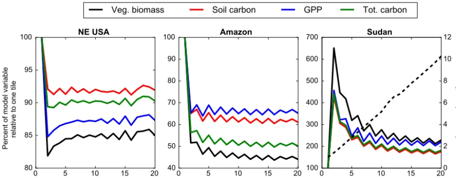
We performed a simple test to ascertain model sensitivity to soil texture, the number of soil tiles, and if this sensitivity has a saturating number of tiles using three example sites: northeast USA (temperate; 43.3◦N, 92.8◦W), the Amazon (tropical;−1.40◦S, 56.25◦W), and the Sudan (arid; 12.6◦N, 28.1◦E). For this test, we first ran a simulation at each test grid cell with a soil texture of 50 % sand and 50 % clay. We then ran different simulations with an increasing number of tiles at each site but with the same proportion of sand and clay percentages for the grid-cell-weighted mean. These fur-ther simulations were (i) two tiles each covering half the grid cell (one with 100 % sand and the other 100 % clay), (ii) three tiles each covering a third (one with 100 % sand, one with 50 % sand and 50 % clay, and the third 100 % clay), (iii) four tiles each covering a fourth (one with 100 % sand, one with 75 % sand and 25 % clay, one with 25 % sand and 75 % clay, and the fourth 100 % clay), (iv) five tiles each covering a fifth (one with 100 % sand, one with 75 % sand and 25 % clay, one with 50 % sand and 50 % clay, one with 25 % sand and 75 % clay, and the fourth 100 % clay), etc. up until 20 tiles. All tiles were assigned the same vegetation, soil depth, and an OM content of 0 %.
Some example carbon cycle outputs are plotted in Fig. 1. As we increase from one tile to two, the model outputs show drops of slightly less than 10 to almost 20 % for the north-east USA and 30 to 50 % at the Amazon site, but show an increase in some variables of up to 6-fold for the Su-dan site. The change in the carbon outputs from the one-tile simulations then decreases and stabilizes, indicating that the model is not sensitive to an increasing number of tiles. The threshold number of tiles at which the carbon outputs stabilize is around 7 or 8 for the northeast USA and Ama-zon while the Sudan site is around 12. The Sudan site has low productivity (net primary productivity, NPP, approxi-mately 300 g C m−2yr−1) due to arid conditions (annual pre-cipitation approximately 400 mm yr−1), and it demonstrates a strong response of the carbon cycle to soil texture. Addi-tionally, since model runtime increases proportionally to the number of tiles (see dashed line in the Sudan plot of Fig. 1), to manage computational cost, only the minimum number of tiles that allows an adequate representation of sub-grid het-erogeneity should be run.
0 5 10 15 20 80
85 90 95 100
Percent of model variable
relative to one tile
NE USA
0 5 10 15 20
Number of tiles 40
50 60 70 80 90
100 Amazon
0 5 10 15 20
100 200 300 400 500 600
700 Sudan
Veg. biomass Soil carbon GPP Tot. carbon
0 2 4 6 8 10 12
Increase in runtime
(multiple of one tile runtime)
Figure 1.Sensitivity test of CLASS-CTEM to the number of tiles (clusters) for three test grid cells. The texture of each tile as the number of tiles increases is described in Sect. 3.1. GPP is gross primary productivity. All simulations were run until a new equilibrium state was established. The increase in runtime of the model is displayed as a dashed line.
3.2 Site-level simulations
3.2.1 Evaluation of soil textural clusters
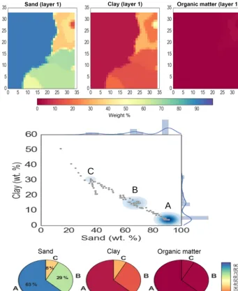
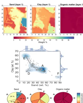
We first examine example grid cells from the Sudan and Brazil (Figs. 2 and 3). These sites were chosen because they are from relatively arid regions, and therefore soil moisture variations should play a role in the vegetation dynamics. Fig-ures 2 and 3 show the high-resolution GSDE grid cell tex-tures for the top CLASS-CTEM soil layer. The clustering algorithm found three clusters for both example grid cells. The weight percent of clay, sand, and OM for each cluster can be seen in Figs. 2 and 3 and compared to the original GSDE grid cells. The joint distribution using kernel density estimation for the sand and clay soil contents is also shown. The clustering is able to effectively capture the distinct soil textural regions apparent in both grid cells. Another example cell with a more heterogeneous GSDE soil texture is shown in Fig. A2.
3.2.2 Influence on model outputs
The CLASS-CTEM simulated net primary productivity (NPP), heterotrophic respiration (HR), and net ecosystem productivity (NEP) for the Sudan and Brazil example sites are shown in Figs. 4 and 5, respectively. Model outputs such as NPP, HR, and NEP are important components of the ter-restrial C cycle but they are also useful indicators of changes in soil hydrology and thermal regimes since their calculation is influenced by the soil environment as a whole. To inves-tigate the influence of the clustering algorithm, the per-tile results are shown alongside the model results taken at the grid level (as a weighted mean) for the clustering simula-tion (“Cluster”) and the model result if a simple mean of the
GSDE soil texture for the CLASS-CTEM grid cell was used (“Gridmean”).
The Sudan grid cell shows relatively large differences be-tween the three tiles determined by the clustering algorithm. The NPP of tile C (with 36 % sand, 31 % clay, and 2 % OM) is generally very low which draws down the grid-level NPP for the Cluster simulation, but not greatly, as this tile only occupies 8 % of the grid cell. The other tiles (A: 91 % sand, 4 % clay, and 1 % OM covering 62 % of the grid cell; B: 67 % sand, 15 % clay, and 1 % OM covering 30 % of the grid cell) can also differ greatly especially for HR and NPP. The NPP and NEP is generally higher for the Gridmean simula-tion while the HR is higher for the Cluster simulasimula-tion. The different sensitivity of CLASS-CTEM’s simulated NPP and HR to each tile’s soil texture is at least partially due to the model formulation of these processes. In CLASS-CTEM, GPP, a component of NPP, depends upon a soil moisture stress term that uses the volumetric water content to deter-mine the degree of soil saturation (Eqs. A5–A7 in Melton and Arora, 2016), whereas the HR calculation depends on soil matric potential (Melton et al., 2015, and Eqs. A33–A36 in Melton and Arora, 2016). Soil matric potential is calcu-lated as
9=9sat
θ
l
θp+θi
−b
, (1)
whereb is the Clapp and Hornbergerb term (Cosby et al., 1984),9satis the soil moisture suction at saturation, andθi,
θl, andθpare the volumetric ice, liquid, and pore (air) content
Figure 2.Example CLASS-CTEM grid cell located in the Sudan (12.6◦N, 28.1◦E). The top panel shows the GSDE sand, clay, and organic carbon weight percents for GSDE cells within the CLASS-CTEM grid cell. Each GSDE grid cell is 5 arcmin by 5 arcmin. The numbers on the plot axes are the number of GSDE grid cells along that axis. The joint distribution using kernel density estimation for the soil sand and clay content is shown in the centre panel. The histograms on the axes and the blue colour scaling demonstrate qualitatively the number of GSDE grid cells sharing the similar soil textural space. The clustering algorithm found three clusters (labelled A, B, and C) with a fractional area per cluster and soil texture as shown in the pie charts. The pie charts can be visually referenced to the top panel which uses the same colour scheme, e.g. cluster A covers 63 % of the CLASS-CTEM grid cell with 91 % sand, 4 % clay, and 1 % OM. In the scatter plot, the label is placed close to the cluster value to help illustrate the cluster relation in sand–clay space.
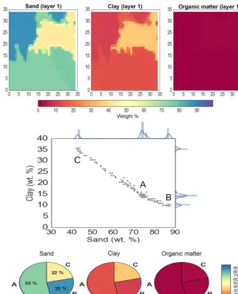
The NPP, HR, and NEP values at the Brazil test site (Fig. 5) are all higher than at the Sudan test site due, in part, to the higher precipitation in the region. The Brazil site’s Gridmean simulation generally has similar NPP and NEP to the Cluster simulation but higher HR. This appears to reflect the relatively similar behaviour between the three tiles deter-mined for this location. The largest difference between tiles is for HR which is lower for tile C (43 % sand, 36 % clay, and 3 % OM) compared to the sandier tiles, A (91 % sand,
4 % clay, and 1 % OM) and B (67 % sand, 15 % clay, and 1 % OM).
Figure 3.Similar to Fig. 2 for a CLASS-CTEM grid cell located in Brazil (9.8◦S, 45.0◦W).
3.3 Global simulations
3.3.1 Evaluation of soil textural clusters
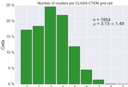
On a global scale, the clustering algorithm found, on aver-age, slightly more than three clusters per CLASS-CTEM grid cell (3.1±1.5; Fig. A3) with few cells having more than five clusters. The global distribution of the number of clusters and the percent of GSDE grid cells that formed the clusters are shown in Fig. 6. The number of clusters found by OPTICS shows a lower number of clusters in parts of the US, Europe, and China, with higher numbers generally found for South America and part of Africa. There appears to be some de-pendence between the number of clusters and the original source soil map that was incorporated into GSDE (see Fig. 1 in Shangguan et al., 2014, for the distribution of source maps
Eu-0 100 200 300 400 500 600 700 NPP (g C m –2
Per tile
A 62 % (91/4/1) B 30 % (67/15/1) C 8 % (36/31/2)
Grid level
Gridmean (75/11/1) Cluster 100 200 300 400 500 600 700Precipitation (
m m y r – 1) Precipitation 0 50 100 150 200 250 300 350 400 450 Heterotrophic respiration (g C m –2 1970197519801985199019952000200520102015 Time 100 0 100 200 300 400 NEP (g C m –2 1970197519801985199019952000200520102015 Time
Sudan (12.6 N 28.1 E)
◦ ◦yr – 1) yr – 1) yr – 1 )
Figure 4.CLASS-CTEM simulated net primary productivity (NPP), heterotrophic respiration, and net ecosystem productivity (NEP; NPP – heterotrophic respiration) for the same grid cell in the Sudan as Fig. 2. The left column shows the model results per tile with soil textures listed as percent sand/clay/OM along with the tile percent grid cell coverage. The right column shows the model results at the grid level for the Cluster simulation (weighted mean average of all tiles) and the Gridmean simulation (simple mean of GSDE soil textures). The annual precipitation for this grid cell from CRU-NCEP is included for reference in the upper right plot.
600 800 1000 1200 1400 1600 1800 N P P Per tile
A 53 % (75/14/1) B 25 % (87/10/1) C 22 % (43/36/3)
Grid level Gridmean (71/18/2) Cluster 600 800 1000 1200 1400 1600 1800 P re ci pi ta tio n ( m m y r – 1) Precipitation 850 900 950 1000 1050 1100 1150 1200 H et er ot ro ph ic R es pi ra tio n (g C m 2
1970197519801985199019952000200520102015
Time 200 0 200 400 600 N E P
1970197519801985199019952000200520102015
Time Brazil (9.8◦S 45.0◦W)
yr – 1) (g C m 2yr – 1) (g C m 2yr – 1)
Number of lusters
Percent in clusters
1 2 3 4 5 6 7 8
10 20 30 40 50 60 70 80 90 100
c
Figure 6.Global distributions of the number of clusters (tiles) found per CLASS-CTEM grid cell (left) and the percent of GSDE grid cells clustered per CLASS-CTEM grid cell (right).
rope could also have higher-quality soil data but it is only a subsection of the European Soils Database. To understand if the selection of the minPts parameter caused the predom-inance of single tiles in these regions, we reduced minPts from 5 to 1 % of the number of data points in the grid cell. This did reduce the number of grid cells with only single tiles in China, the US, and Europe, but it also greatly increased the number of tiles everywhere else (Fig. A4). The mean num-ber of clusters found increased to 11.2±5.2 with some grid cells having up to 20 cells. Since the model is not sensitive to more than about seven tiles (see Sect. 3.1), the original minPts value used appears more appropriate for the majority of the land surface.
The percent of GSDE grid cells that were included in clus-ters is, on average, 57.0±20.1, as not all GSDE soil textu-ral values are necessarily determined to fall within a cluster (as discussed in Sect. 2.3.1). The clustering does not, how-ever, appreciably shift the simple grid-mean texture of the CLASS-CTEM grid cells (Figs. A5 and A6); i.e. the raw Gridmean is similar to the weighted mean of the clusters. The spatial distribution of the percent of GSDE cells clustered is shown in Fig. 6. Areas of northern Eurasia, southeastern Aus-tralia, and the prairie region of Canada appear to have lower percentages of GSDE grid cells clustered, while areas like northern Africa and the high latitudes of Canada have higher percentages clustered although the pattern on the whole is relatively heterogeneous.
3.3.2 Influence on model outputs
Global totals of CLASS-CTEM outputs for tiled (Cluster) and grid-mean (Gridmean) simulations for 1996–2015, along with observation-based estimates, are presented in Table 1. The general impact of the clustering integrated over the globe is small for most variables. Evapotranspiration (ET), transpi-ration, and runoff show small differences of around 1 % or less. There are some seasonal and regional differences for ET between the Cluster and Gridmean simulations (Fig. A7) but
they are generally not statistically significant (independent two-sample t-test p level<0.01). The transpiration com-ponent of ET is relatively unchanged globally between the Cluster and Gridmean simulations (Table 1) while changes at the grid cell level indicate a partitioning shift between evapo-ration and transpievapo-ration with some arid regions showing more transpiration for the Cluster simulations (Figs. A8 and A7). Runoff also has some seasonal differences with more grid cells significantly different between Cluster and Gridmean simulations (Fig. A9) and while the Cluster simulation has generally higher runoff, the signal is quite mixed. Globally, latent heat fluxes are less influenced by the tiling than sen-sible heat fluxes with a 0.4 % difference compared to 3.7 %, respectively. Seasonal maps of latent heat fluxes show little difference between the two simulations (not shown) while there is a general increase in sensible heat fluxes of the Clus-ter simulation over the Gridmean for all seasons in arid re-gions (Fig. A10).
Some variables for the carbon cycle also show similar relatively small changes with the largest changes occurring for NEP with a 4 % difference between simulations and net biome productivity (NBP) with a 5 % difference. The largest difference is observed for water use efficiency (WUE; de-fined as GPP/ET) with a percent absolute difference of about 33 %. The higher mean annual global WUE of the Cluster simulation is also closer to an observation-based estimate (Xue et al., 2015) than the Gridmean simulation. The change in WUE between the two simulations will be discussed in greater detail below.
north-Soil layer 1 (0–0.1 m) Soil layer 2 (0.1–0.35 m) Soil layer 3 (0.35–4.1 m)
20 12 8 5 3 3 5 8 12 20
Percent difference relative to gridmean ([(cluster – gridmean) / gridmean] * 100)
Figure 7.Percent difference in soil moisture per CLASS-CTEM soil layer between the Cluster and Gridmean simulations (mean of 1995–
2015). Grid cells with soil moisture below 10−5kg m−2were masked out to prevent instances of division by zero and overly large relative
differences in regions of very little soil moisture. Positive values indicate the Cluster soil moisture is larger while negative values indicate the
Gridmean soil moisture is larger. Dots indicate grid cells that are statistically significant (independent two-samplet-testplevel<0.01).
Table 1.Global annual values for CLASS-CTEM model outputs based on simulations using grid-mean soil textures (Gridmean) and tiled simulations derived from the clustering analysis (Cluster). Values are an average over the period 1996–2015.
CLASS-CTEM output Cluster Gridmean Percent absolute Observation-based estimate
difference
Evapotranspiration (ET; 103km3yr−1) 78.3 78.6 0.5 83.9±9.9 (Trenberth et al., 2011)a
Transpiration (T; 103km3yr−1) 21.1 21.2 0.3 62±8 (Jasechko et al., 2013),
45±4.5 (Schlesinger and Jasechko, 2014)
T /ET (%) 27.0 27.0 0.1 61±15(Schlesinger and Jasechko, 2014)
Runoff (103km3yr−1) 32.8 32.4 1.1 38.3 (Fekete et al., 2002)
Latent heat fluxes (W m−2) 44.9 45.2 0.4 39±2 (Jung et al., 2011),
38.5 (Trenberth et al., 2009) 37–59 (Jiménez et al., 2011)
Sensible heat fluxes (W m−2) 25.5 24.6 3.7 41±4 (Jung et al., 2011),
27 (Trenberth et al., 2009) 18–57 (Jiménez et al., 2011)
Water use efficiency (g C kg−1water) 1.47 1.10 32.8 1.70 (Xue et al., 2015)
Gross primary productivity (GPP) (Pg C yr−1) 133.1 133.6 0.4 123±8 (Beer et al., 2010)
Vegetation biomass (Pg C) 555.00 558.46 0.6 300–536 (Forest biomass)b
Soil carbon mass (Pg C) 1132.1 1119.6 1.1 1922c(Shangguan et al., 2014)
Area burnt (104km2yr−1) 484 505 4.2 464 (Randerson et al., 2012)
Net ecosystem productivity (NEP) (Pg C yr−1) 4.6 4.8 4.0
Net biome productivity (NBP) (Pg C yr−1) 1.0 1.1 5.0 1.0–2.5d(Le Quéré et al., 2016)
Percent absolute difference is calculated as abs{100− [(clustered value/grid-mean value)×100]}.
aValue from eight reanalyses for 2002–2008, except ERA-40 which was for the 1990s. bAs summarized in Kauppi (2003).
cNote that this version of CLASS-CTEM does not simulate permafrost C pools. dRange of all estimates across the 1990–2015 time period.
ern Australia, the Middle East, and Mongolia (which have low soil moisture, so small changes in absolute amounts will appear as a larger percent change than the same absolute change in a more humid region), while the northern latitudes are wetter for some of the Canadian high north and western Siberia as well as areas of Indonesia and other parts of south-east Asia. These patterns are not uniform and can also differ by soil model layer as is the case in the Saharan region where the second layer is generally wetter for the Cluster simulation than for the Gridmean but drier in the third layer. The drier
first soil layer in the Cluster simulations leads to an increase in sensible heat fluxes over the Gridmean simulations as seen in Fig. A10 and Table 1.
Gridmean
Beer et al. (2010)
300 600 900 1200 1500 1800 2100 2400 2700
kg C m
−
2
(Cluster - gridmean) / gridmean * 100
40 0 40 80 120 160 200 240
Percent
(a) (b)
(d)
(c)
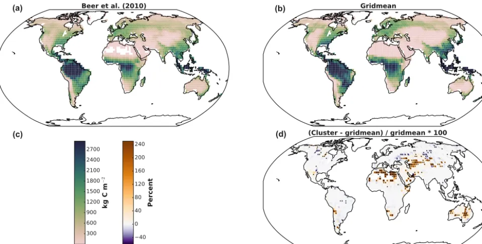
Figure 8. Mean annual gross primary productivity (1982–2008) from an observation-based dataset (Beer et al., 2010)(a), the Gridmean
simulation(b), and percent relative difference between the Cluster and Gridmean simulations(d). Note that many of the regions with the
largest changes in GPP between the two approaches are also regions with low GPP; hence, the absolute change in GPP is generally small.
Dots indicate grid cells that are statistically significant (independent two-samplet-testplevel<0.01). For the areas of significant change
in GPP between the Cluster and Gridmean simulations, comparison of Cluster and Gridmean simulations against observations was not significant after accounting for the observational uncertainty.
OM≥30 %; see Sect. 2.1). The higher porosity, greater hy-draulic conductivity variation with depth, and differing ther-mal properties all cause greater changes in soil moisture when a grid cell or tile is treated as peat soil as opposed to a mineral soil. The differences in soil moisture appear to be relatively stable throughout the year with relatively little sea-sonal variation (not shown).
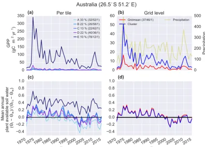
Changes in soil moisture will influence vegetation through changes in water supply and water stress. The mean annual gross primary productivity (GPP) as simulated by CLASS-CTEM is plotted in Fig. 8. An observation-based estimate (Beer et al., 2010) is provided for reference against the Grid-mean simulation GPP. The relative percent difference be-tween the Gridmean and Cluster simulations can be large in arid regions while relatively small elsewhere (again with the understanding that small absolute changes appear rela-tively larger for areas of low GPP than for the same abso-lute change in a region of higher productivity). The areas of significant difference are similar to the regions that saw the significant changes in total soil moisture (Fig. 7) includ-ing central Australia, Saharan Africa, and other arid regions. In these arid regions, the Cluster simulation produces higher GPP values than the Gridmean simulation. However, in these regions, the soil moisture in the total soil column was less in the Cluster simulation than in the Gridmean simulation (with the exception of Saharan Africa where the second soil layer
increased in soil moisture). In non-arid regions, the general effect of the clustering was to slightly lower GPP (resulting in a slightly smaller global GPP; Table 1). Regions like the peat-land complexes that showed significant changes in soil mois-ture (Fig. 7) are already moist and rarely experience water stress; thus, these changes in soil moisture have little impact upon productivity. We investigated the temporal dynamics of GPP in the regions that differed significantly between the Cluster and Gridmean simulations using the dataset of Jung et al. (2011) and found a small improvement in root mean square deviation of the cluster simulation over the Gridmean, but it was smaller than the uncertainty of the Jung et al. (2011) dataset which is relatively large in these regions due to sparse observations (e.g. Fig. S2 in Beer et al., 2010) and low productivity.
0 50 100 150 200 250 300 350 GPP (gC m yr ) –2 Per tile
A 33 % (32/52/1) B 22 % (26/58/1) C 13 % (22/62/1) D 22 % (40/36/1) E 10 % (78/12/1)
0 10 20 30 40 50
60 Grid level
Gridmean (37/46/1) Cluster 0 100 200 300 400 500
Precipitation (mm
yr Precipitation 1970197519801985199019952000200520102015 Time 0.4 0.2 0.0 0.2 0.4 0.6 0.8 1.0 Mean annual
plant available soil water ( Θl − Θw )/ (Θ fc − Θw ) 1970197519801985199019952000200520102015 Time 0.4 0.2 0.0 0.2 0.4 0.6 0.8 1.0
Australia (26.5
◦S 51.2
◦E)
–1 ) –1 (a) (b) (d) (c)
Figure 9.Australian grid cell that has higher GPP for the Cluster simulation than the Gridmean simulation, but lower soil moisture. A measure of the mean annual plant-available soil water, scaled so that 1 indicates field capacity and 0 is the wilting point, is calculated for the second model soil layer (0.1–0.35 m) and is described in Sect. 3.3.2. The annual precipitation for this grid cell from CRU-NCEP is included for
reference in panel(b).
soil’s field capacity,θfc, and wilting point,θw:
θa=θfc−θw. (2)
The GPP formulation of CLASS-CTEM is sensitive to θa
(Melton and Arora, 2016) and thus enforces stomatal closing to limit water loss during periods of low moisture availability, resulting in lower productivity. From Fig. 9, we can see tile E, on an annual basis, generally has some plant-available wa-ter while the other tiles, and Cluswa-ter-weighted mean (Fig. 9d) and the Gridmean simulation, are commonly strongly water limited resulting in higher GPP for tile E than other tiles and the Gridmean simulation.
The large changes in the global mean WUE seen in Table 1 can also be observed regionally and seasonally (Fig. A11). Outside of arid regions, the Gridmean simula-tion has a slightly higher WUE, although it is generally not statistically significant. Arid regions show greatly increased WUE principally due to the higher GPP discussed previously (Fig. 8), while the increase in evapotranspiration is muted by a compensating shift in transpiration versus evaporation as discussed above; thus, while the effect of tiling on WUE ap-pears larger than other variables, some of the impact is sim-ply due to how WUE is formulated (ratio of two variables
and commonly given as a global mean value, not a global sum) and its sensitivity to small changes in its components.
The large influence of the clustering in arid regions demonstrates the impact of soil texture when water limita-tions are important. In these arid regions, the amount of water in the soil column is low, and thus soil textural changes that allow greaterθa are important, while regions with plentiful
moisture are much less influenced by soil texture since water stress is less frequent and the soils generally contain suffi-cient water for photosynthesis. CLASS-CTEM’s pedotrans-fer functions could also be limiting the influence of the tiling of soil textures. The range inθafor the Cosby et al. (1984)
pe-dotransfer functions, as implemented in CLASS-CTEM, for soils ranging from the most disparate USDA texture classes (“sand” to “silt” to “clay”) only covers aθarange of 0.08.
Us-ing another pedotransfer function may cause CLASS-CTEM to have a greater sensitivity to soil textural changes. For ex-ample, the range inθa using the Saxton and Rawls (2006)
pedotransfer functions is over double the range of CLASS-CTEM’s implementation of Cosby et al. (1984) (θa high to
tex-tures (Fig. A5). Additionally, the GPP moistustress re-sponse of CLASS-CTEM could be quite different from an-other model; thus, the effects could be somewhat dependent upon the model used.
4 Conclusions and future work
Soil texture influences soil hydrology and temperature and is commonly assigned simple mean values across large grid cells. The sub-grid heterogeneity of soil texture can be rep-resented by tiling of the land surface. To test the sensitivity of our model, CLASS-CTEM, to soil texture, we ran simula-tions of three artificial test grid cells with increasing numbers of tiles but the same grid-mean soil texture. CLASS-CTEM’s carbon cycle outputs were sensitive to the tiling with some outputs changing greatly but displaying a saturating effect dependent upon the climate of the grid cell that ranged be-tween 7 and 12 tiles. We then used two linked clustering algorithms – the OPTICS algorithm (Ankerst et al., 1999; Daszykowski et al., 2002) and the algorithm of Sander et al., 2003 – to cluster high-resolution soil textures over the rela-tively coarse CLASS-CTEM model grid (approximately 2.8◦ by 2.8◦). After determining the impact of this tiling at two locations, we ran global simulations using tiled soil textures against those with a simple grid-mean soil texture. The dif-ference between the two simulations on a global scale were generally relatively small (<5 %) but could be large region-ally (>20 %). The areas that felt the largest impact due to the soil texture tiling were in arid or peatland regions. Peatland regions were more sensitive to the tiling due to the model pa-rameterization of peatland soils, that is subject to a minimum organic matter limit, and which could be exceeded for single tiles while the simple grid mean remained below the limit. Arid regions saw the largest impact upon GPP due to those regions’ general state of moisture stress on the vegetation, whereas the peatland regions generally have abundant soil moisture. Tiles that retained higher levels of plant-available water in arid regions would greatly increase GPP causing the grid-level GPP to rise above that simulated when using a sim-ple grid-mean soil texture.
In water-limited regions, the inverse-texture hypothesis as put forth by Noy-Meir (1973) and Sala et al. (1997) predicts that coarse-textured soils will support higher above-ground plant net primary productivity than fine-textured soils. This hypothesis has been supported by observations across
pre-cipitation gradients (Lane et al., 1998), and we also find this in our simulations for semi-arid and arid regions (Figs. 4, 5, and 9). The role of soil texture is even stronger on plant community composition based on both observations (Lane et al., 1998; Dodd et al., 2002; Dodd and Lauenroth, 1997; Fernandez-Illescas et al., 2001) and modelling stud-ies (Bucini and Hanan, 2007). While our model does have a parameterization for competition between plants for ground coverage (Melton and Arora, 2016), we do not presently have shrub PFTs. As the major interactions in these regions is be-tween grasses and shrubs, our competition parameterization is unlikely to appropriately capture the dynamics of plant cover due to soil texture as has been reported by observa-tional studies.
We suggest the following as some possible future direc-tions for this work. First, mapping of the PFTs so the PFTs observed for each point in the GSDE grid are assigned to the same tile as their underlying soil textures. Presently, we give all tiles in the grid cell the same composition of PFTs, whereas the underlying soil conditions could lead to notable differences in which PFTs exist in a location. Second, the Zobler (1986) soil depth dataset is markedly shallow com-pared to a more recent dataset (Pelletier et al., 2016). In-troducing the newer soil dataset into the clustering could al-low greater distinction of clusters within a tile, e.g. river val-leys with deep soil columns with surrounding shallow soil uplands. Lastly, the use of different pedotransfer functions could yield more model sensitivity to the clustering. An ex-amination of pedotransfer functions would need to look care-fully at the impact of the function for test sites with well-understood soil conditions.
While the performance of the tiled grid cells in the arid re-gions is encouraging, the overall impact of tiling on the ter-restrial C cycle is relatively small, and thus the use of a sim-ple grid-mean soil texture is likely sufficient for most appli-cations. For large-scale applications with a special interest in arid regions, selectively tiling those regions could be useful for capturing the impact of soil heterogeneity on plant pro-ductivity.
Code availability. The Python code used for the OPTICS and
Appendix A: CLASS-CTEM soil pedotransfer functions Figure A12 demonstrates the non-linear relationships be-tween soil texture and the hydrologic soil state variables. The saturated hydraulic conductivity,Ksat(m s−1; Fig. A12),
is found from the weight percentage sand content,Xsand, as
(Cosby et al., 1984; Verseghy, 2012)
Ksat=7.0556×10⁻⁶exp(0.0352Xsand−2.035) , (A1)
while the pore volume,θp(m3m−3; Fig. A12), is also
calcu-lated usingXsand(Cosby et al., 1984; Verseghy, 2012):
θp=(−0.126Xsand+48.9) /100.0. (A2)
The soil moisture suction at saturation, 9sat(m; Fig. A12),
usesXsand:
9sat=0.01 exp(−0.0302Xsand+4.33) . (A3)
The hydraulic parameter b (unitless; also called the Clapp and Hornbergerbterm) is calculated via the weight percent-age clay content,Xclay(Cosby et al., 1984; Verseghy, 2012),
as
b=0.159Xclay+2.91. (A4)
The hydraulic conductivity of the soil, K (m s−1), is then related to the soil’s volumetric liquid water content, θl
(m3m−3), via the Clapp and Hornberger (1978) relationship:
K=Ksat θl/θp(2b
+3)
. (A5)
In CLASS-CTEM, the field capacity of soil moisture, θfc
(m3m−3; Fig. A12), is found by setting K in Eq. (A5) to 0.1 mm d−1(1.157×10⁻⁹mm s−1) and then solving for the liquid water content:
θfc=θp
1.157×10⁻⁹/Ksat
1/(2b+3)
. (A6)
The field capacity of the lowest permeable layer, θfc, b
(m3m−3), accounts for the permeable depth of the whole
overlying soil column,zb(m), and is found via Soulis et al.
(2011):
θfc, b=θp/(b−1)(9satb/zb)1/b(3b+2)(b−1)/b
−(2b+2)(b−1)/b. (A7)
At the wilting point, the soil moisture suction,9wilt, is set to
150 m. The volumetric water content at the wilting point,θw
(m3m−3), is then calculated as
θw=θp(9wilt/9sat)1/b. (A8)
The thermal regime of the soil is also influenced by soil tex-ture. The volumetric heat capacity of soils in CLASS-CTEM,
Cg(J m−3K−1) is derived from the volume fraction (V) and
volumetric heat capacity of clay and silt,Cfine, sand,Csand,
and organic matter (OM),COM, components of the soil
ma-trix as a weighted average:
Cg=6(CsandVsand+CfineVfine+COMVOM)/(1−θp). (A9)
In a similar manner, the soil thermal conductivity, τg
(W m−1K−1), is calculated via a weighted average of the
components’ thermal conductivities:
τg=6(τsandVsand+τfineVfine+τOMVOM)/(1−θp). (A10)
Organic soils, defined as those cells having an organic matter weight percent greater than 30, are assigned values ofKsat,
θp,θfc,9sat,b,K,Cg, andτgbased on peat texture following
Number of clusters
1
2
3
4
5
6
7
8
Figure A1.Map of the number of clusters for all CLASS-CTEM grid cells where the weighted mean of the clusters was more than 10 % different than the simple mean of all GSDE grid cells within a CLASS-CTEM grid cell. These grid cells were then assigned the simple Gridmean soil texture values for all simulations (see Sect. 2.3.1).
1 2 3 4 5 6 7 8 9 0 %
5 % 10 % 15 % 20 % 25 %
Cells
n = 1954
µ
= 3.13
±1.49
Number of clusters per CLASS-CTEM grid cell
Figure A3.Number of clusters determined per CLASS-CTEM grid cell for the GSDE (Shangguan et al., 2014) dataset.
Number of clusters
1 2 3 4 5 6 7 8 > 8
Figure A4.Global distributions of the number of clusters (tiles) found per CLASS-CTEM grid cell when minPts (see Sect. 2.3) is set to 1 % of the number of GSDE data points in the CLASS-CTEM grid cell. The gray regions have more than eight tiles found by the clustering algorithms.
Figure A6.Histogram of the difference between the mean clay, sand, and organic matter content for CLASS-CTEM grid cells based on the simple mean value of all GSDE cells and the weighted mean of the clusters within a CLASS-CTEM grid cell.
DJF
MAM
JJA
SON
15 10 5 3 1 1 3 5 10 15
Percent difference relative to gridmean [(clustered - gridmean) / gridmean] * 100
Figure A7.Percent difference in evapotranspiration (ET) between the Cluster and Gridmean simulations by season (mean of 1995–2015).
Grid cells with monthly ET of<10−5mm water were masked out to prevent instances of division by zero and overly large relative differences
in regions of very small evapotranspiration. Positive values indicate the Cluster simulation ET is larger while negative values indicate the
DJF
MAM
JJA
SON
25 15 10 5 3 3 5 10 15 25
Percent difference relative to gridmean [(clustered - gridmean) / gridmean] * 100
Figure A8.Percent difference in transpiration between the Cluster and Gridmean simulations by season (mean of 1995–2015) following Fig. A7.
DJF
MAM
JJA
SON
25 15 10 5 3 3 5 10 15 25
Percent difference relative to gridmean [(clustered - gridmean) / gridmean] * 100
DJF
MAM
JJA
SON
25 15 10 5 3 3 5 10 15 25
Percent difference relative to gridmean [(clustered - gridmean) / gridmean] * 100
Figure A10. Percent difference in sensible heat fluxes between the Cluster and Gridmean simulations by season (mean of 1995–2015) following Fig. A7.
DJF
MAM
JJA
SON
100 50 20 10 5 5 10 20 50 100
Percent difference relative to gridmean [(clustered - gridmean) / gridmean] * 100
Figure A11.Percent difference in WUE between the Cluster and Gridmean simulations by season (mean of 1995–2015). Grid cells with
monthly evapotranspiration of<10−5mm water were masked out to prevent instances of division by zero and overly large relative
dif-ferences in regions of very small evapotranspiration. Positive values indicate the Cluster WUE is larger while negative values indicate the
Sand (wt. %) 0 20 40 60 80 100
Clay (wt. %) 0 20 40 60 80 100
Θfc
0.10 0.15 0.20 0.25 0.30 0.35 0.40 0.45
0 20 40 60 80 100
Sand (wt. %) 0.36
0.38 0.40 0.42 0.44 0.46 0.48 0.50
Θ
p(
m
3m -3)
0 20 40 60 80 100
Clay (wt. %) 0.000000
0.000005 0.000010 0.000015 0.000020 0.000025 0.000030 0.000035
K
sat
(
m
s
)
0 20 40 60 80 100
Sand (wt. %) 0.0
0.1 0.2 0.3 0.4 0.5 0.6 0.7 0.8
ψ
sat
(m)
-1
(a) (b)
(c) (d)
Figure A12.Relationships between soil texture and field capacity (θfc;a), pore volume (θp;b), saturated hydraulic conductivity (Ksat;c),
Author contributions. JRM initiated the study, performed the clus-tering, ran the model simulations, performed the analysis, and wrote the first draft of the paper. KEM suggested clustering analysis, pro-vided coding help for the Python scripts as well as interpretation and statistical assistance. RSA helped choose clustering algorithms, compared results to observations, and helped determine CLASS-CTEM’s sensitivity to the number of clusters. All authors con-tributed to the final paper.
Competing interests. The authors declare that they have no conflict
of interest.
Acknowledgements. Reinel Sospedra-Alfonso was supported by
a Natural Sciences and Engineering Research Council of Canada (NSERC) Visiting Fellowship. Kelly E. McCusker was supported by the CanSISE Network, which is funded by the NSERC under the Climate Change and Atmospheric Research (CCAR) programme. We thank Michal Daszykowski for sharing his coding of the OPTICS algorithm and Brian H. Clowers for sharing his porting of this code into Python. We also thank Amy X. Zhang for sharing her Python code implementing the algorithm of Sander et al. (2003). The high-resolution soil textural database was kindly shared by Wei Shangguan. We thank Vivek Arora and Christian Seiler for providing comments on an earlier version of the manuscript. We also thank our four reviewers (Hui Zheng, Eleanor Blyth, and two anonymous reviewers) for their comments which improved our manuscript.
Edited by: Min-Hui Lo
Reviewed by: Eleanor Blyth, Hui Zheng, and two anonymous referees
References
Ankerst, M., Breunig, M. M., Kriegel, H.-P., and Sander, J.: OP-TICS: Ordering Points to Identify the Clustering Structure, in: Proceedings of the 1999 ACM SIGMOD International Confer-ence on Management of Data, SIGMOD ’99, ACM, New York, NY, USA, 49–60, https://doi.org/10.1145/304182.304187, 1999. Archer, N. A. L., Quinton, J. N., and Hess, T. M.: Below-ground relationships of soil texture, roots and hydraulic conductivity in two-phase mosaic vegetation in South-east Spain, J. Arid Envi-ron., 52, 535–553, https://doi.org/10.1006/jare.2002.1011, 2002. Archibald, S., Lehmann, C. E. R., Gómez-Dans, J. L., and Bradstock, R. A.: Defining pyromes and global syndromes of fire regimes, P. Natl. Acad. Sci. USA, 110, 6442–6447, https://doi.org/10.1073/pnas.1211466110, 2013.
Arora, V. K., Chiew, F. H. S., and Grayson, R. B.: Effect of sub-grid-scale variability of soil moisture and precipitation intensity on surface runoff and streamflow, J. Geophys. Res., 106, 17073– 17091, https://doi.org/10.1029/2001JD900037, 2001.
Avissar, R. and Pielke, R. A.: A parameterization of
het-erogeneous land surfaces for atmospheric numerical
models and its impact on regional meteorology, Mon. Weather Rev., 117, 2113–2136, https://doi.org/10.1175/1520-0493(1989)117<2113:APOHLS>2.0.CO;2, 1989.
Bartholomé, E., and Belward, A. S.: GLC2000: a new ap-proach to global land cover mapping from Earth
ob-servation data, Int. J. Remote Sens., 26, 1959–1977,
https://doi.org/10.1080/01431160412331291297, 2005. Beer, C., Reichstein, M., Tomelleri, E., Ciais, P., Jung, M.,
Car-valhais, N., Rödenbeck, C., Arain, M. A., Baldocchi, D., Bo-nan, G. B., Bondeau, A., Cescatti, A., Lasslop, G., Lindroth, A., Lomas, M., Luyssaert, S., Margolis, H., Oleson, K. W., Roup-sard, O., Veenendaal, E., Viovy, N., Williams, C., Wood-ward, F. I., and Papale, D.: Terrestrial gross carbon dioxide up-take: global distribution and covariation with climate, Science, 329, 834–838, https://doi.org/10.1126/science.1184984, 2010. Boone, A. and Wetzel, P. J.: A simple scheme for modeling sub-grid
soil texture variability for use in an atmospheric climate model, J. Meteorol. Soc. Jpn., 77, 317–333, 1999.
Bucini, G. and Hanan, N. P.: A continental-scale analysis of tree cover in African savannas, Glob. Ecol. Biogeogr., 16, 593–605, 2007.
Chiang, M. M.-T. and Mirkin, B.: Intelligent choice of the
number of clusters in k-means clustering: an experimental
study with different cluster spreads, J. Classif., 27, 3–40, https://doi.org/10.1007/s00357-010-9049-5, 2010.
Clapp, R. B. and Hornberger, G. M.: Empirical equations for some soil hydraulic properties, Water Resour. Res., 14, 601–604, https://doi.org/10.1029/WR014i004p00601, 1978.
Cosby, B. J., Hornberger, G. M., Clapp, R. B., and Ginn, T. R.: A statistical exploration of the relationships of soil moisture char-acteristics to the physical properties of soils, Water Resour. Res., 20, 682–690, https://doi.org/10.1029/WR020i006p00682, 1984. Daszykowski, M., Walczak, B., and Massart, D. L.: Looking for natural patterns in analytical data. 2. Tracing local den-sity with OPTICS, J. Chem. Inf. Comp. Sci., 42, 500–507, https://doi.org/10.1021/ci010384s, 2002.
Decharme, B. and Douville, H.: Introduction of a sub-grid hydrol-ogy in the ISBA land surface model, Clim. Dynam., 26, 65–78, https://doi.org/10.1007/s00382-005-0059-7, 2005.
Dirmeyer, P. A., Dolman, A. J., and Sato, N.: The pi-lot phase of the global soil wetness project, B. Am. Meteorol. Soc., 80, 851–878, https://doi.org/10.1175/1520-0477(1999)080<0851:TPPOTG>2.0.CO;2, 1999.
Dodd, M. B. and Lauenroth, W. K.: The influence of soil texture on the soil water dynamics and vegetation structure of a shortgrass steppe ecosystem, Plant Ecol., 133, 13–28, https://doi.org/10.1023/A:1009759421640, 1997.
Dodd, M. B., Lauenroth, W. K., Burke, I. C., and Chap-man, P. L.: Associations between vegetation patterns and soil texture in the shortgrass steppe, Plant Ecol., 158, 127–137, https://doi.org/10.1023/A:1015525303754, 2002.
English, N. B., Weltzin, J. F., Fravolini, A., Thomas, L., and Williams, D. G.: The influence of soil texture and
vegetation on soil moisture under rainout shelters in
a semi-desert grassland, J. Arid Environ., 63, 324–343, https://doi.org/10.1016/j.jaridenv.2005.03.013, 2005.
Essery, R. L. H., Best, M. J., Betts, R. A., Cox, P. M.,
and Taylor, C. M.: Explicit representation of subgrid
heterogeneity in a GCM land surface scheme, J.
Hy-drometeorol., 4, 530–543,
Famiglietti, J. S. and Wood, E. F.: Multiscale modeling of spatially variable water and energy balance processes, Water Resour. Res., 30, 3061–3078, https://doi.org/10.1029/94WR01498, 1994. Fekete, B. M., Vörösmarty, C. J., and Grabs, W.: High-resolution
fields of global runoff combining observed river discharge and simulated water balances, Global Biogeochem. Cy., 16, 1042, https://doi.org/10.1029/1999GB001254, 2002.
Fernandez-Illescas, C. P., Porporato, A., Laio, F., and Rodriguez-Iturbe, I.: The ecohydrological role of soil texture in a water-limited ecosystem, Water Resour. Res., 37, 2863–2872, 2001. Hook, P. B. and Burke, I. C.: Biogeochemistry in a shortgrass
land-scape: control by topography, soil texture, and microclimate, Ecology, 81, 2686–2703, https://doi.org/10.2307/177334, 2000. Hurtt, G. C., Chini, L. P., Frolking, S., Betts, R. A., Feddema, J.,
Fischer, G., Fisk, J. P., Hibbard, K., Houghton, R. A., Jane-tos, A., Jones, C. D., Kindermann, G., Kinoshita, T., Gold-ewijk, K. K., Riahi, K., Shevliakova, E., Smith, S., Stehfest, E., Thomson, A., Thornton, P., van Vuuren, D. P., and Wang, Y. P.: Harmonization of land-use scenarios for the period 1500–2100: 600 years of global gridded annual land-use transitions, wood harvest, and resulting secondary lands, Clim. Change, 109, 117– 161, https://doi.org/10.1007/s10584-011-0153-2, 2011. Jasechko, S., Sharp, Z. D., Gibson, J. J., Birks, S. J., Yi, Y., and
Fawcett, P. J.: Terrestrial water fluxes dominated by transpira-tion, Nature, 496, 347–350, https://doi.org/10.1038/nature11983, 2013.
Jiménez, C., Prigent, C., Mueller, B., Seneviratne, S. I., Mc-Cabe, M. F., Wood, E. F., Rossow, W. B., Balsamo, G., Betts, A. K., Dirmeyer, P. A., Fisher, J. B., Jung, M., Kanamitsu, M., Reichle, R. H., Reichstein, M., Rodell, M., Sheffield, J., Tu, K., and Wang, K.: Global intercomparison of 12 land surface heat flux estimates, J. Geophys. Res., 116, D02102, https://doi.org/10.1029/2010JD014545, 2011.
Jung, M., Reichstein, M., Margolis, H. A., Cescatti, A., Richard-son, A. D., Arain, M. A., Arneth, A., Bernhofer, C., Bonal, D., Chen, J., Gianelle, D., Gobron, N., Kiely, G., Kutsch, W., Lasslop, G., Law, B. E., Lindroth, A., Merbold, L., Montagnani, L., Moors, E. J., Papale, D., Sottocornola, M., Vaccari, F., and Williams, C.: Global patterns of land-atmosphere fluxes of carbon dioxide, latent heat, and sensi-ble heat derived from eddy covariance, satellite, and meteoro-logical observations, J. Geophys. Res.-Biogeo., 116, G00J07, https://doi.org/10.1029/2010JG001566, 2011.
Kauppi, P.: New, low estimate for carbon stock in global forest vegetation based on inventory data, Silva Fenn., 37, 451–457, https://doi.org/10.14214/sf.484, 2003.
Ke, Y., Leung, L. R., Huang, M., and Li, H.: Enhancing the representation of subgrid land surface characteristics in land surface models, Geosci. Model Dev., 6, 1609–1622, https://doi.org/10.5194/gmd-6-1609-2013, 2013.
Koster, R. D. and Suarez, M. J.: A comparative analy-sis of two land surface heterogeneity representations, J.
Climate, 5, 1379–1390,
https://doi.org/10.1175/1520-0442(1992)005<1379:ACAOTL>2.0.CO;2, 1992.
Kumar, J., Mills, R. T., Hoffman, F. M., and Hargrove, W. W.:
Par-allel k-means clustering for quantitative ecoregion delineation
using large data sets, Procedia Comput. Sci., 4, 1602–1611, https://doi.org/10.1016/j.procs.2011.04.173, 2011.
Landry, J.-S., Ramankutty, N., and Parrott, L.: Investigating the ef-fects of subgrid cell dynamic heterogeneity on the large-scale modeling of albedo in boreal forests, Earth Interact., 20, 1–23, https://doi.org/10.1175/EI-D-15-0022.1, 2016.
Lane, D. R., Coffin, D. P., and Lauenroth, W. K.: Effects of soil tex-ture and precipitation on above-ground net primary productivity and vegetation structure across the Central Grassland region of the United States, J. Veg. Sci., 9, 239–250, 1998.
Le Quéré, C., Andrew, R. M., Canadell, J. G., Sitch, S., Kors-bakken, J. I., Peters, G. P., Manning, A. C., Boden, T. A., Tans, P. P., Houghton, R. A., Keeling, R. F., Alin, S., Andrews, O. D., Anthoni, P., Barbero, L., Bopp, L., Chevallier, F., Chini, L. P., Ciais, P., Currie, K., Delire, C., Doney, S. C., Friedlingstein, P., Gkritzalis, T., Harris, I., Hauck, J., Haverd, V., Hoppema, M., Klein Goldewijk, K., Jain, A. K., Kato, E., Körtzinger, A., Land-schützer, P., Lefèvre, N., Lenton, A., Lienert, S., Lombardozzi, D., Melton, J. R., Metzl, N., Millero, F., Monteiro, P. M. S., Munro, D. R., Nabel, J. E. M. S., Nakaoka, S.-I., O’Brien, K., Olsen, A., Omar, A. M., Ono, T., Pierrot, D., Poulter, B., Röden-beck, C., Salisbury, J., Schuster, U., Schwinger, J., Séférian, R., Skjelvan, I., Stocker, B. D., Sutton, A. J., Takahashi, T., Tian, H., Tilbrook, B., van der Laan-Luijkx, I. T., van der Werf, G. R., Viovy, N., Walker, A. P., Wiltshire, A. J., and Zaehle, S.: Global Carbon Budget 2016, Earth Syst. Sci. Data, 8, 605–649, https://doi.org/10.5194/essd-8-605-2016, 2016.
Letts, M. G., Roulet, N. T., Comer, N. T., Skarupa, M. R., and Verseghy, D. L.: Parametrization of peatland hydraulic properties for the Canadian land surface scheme, Atmos. Ocean, 38, 141– 160, https://doi.org/10.1080/07055900.2000.9649643, 2000. Li, R. and Arora, V. K.: Effect of mosaic representation of
vegeta-tion in land surface schemes on simulated energy and carbon bal-ances, Biogeosciences, 9, 593–605, https://doi.org/10.5194/bg-9-593-2012, 2012.
Li, Y., Shi, Z., Li, F., and Li, H.-Y.: Delineation of site-specific management zones using fuzzy clustering analysis in a coastal saline land, Comput. Electron. Agr., 56, 174–186, https://doi.org/10.1016/j.compag.2007.01.013, 2007.
Meinshausen, M., Smith, S. J., Calvin, K., Daniel, J. S.,
Kainuma, M. L. T., Lamarque, J.-F., Matsumoto, K.,
Montzka, S. A., Raper, S. C. B., Riahi, K., Thomson, A., Velders, G. J. M., and van Vuuren, D. P.: The RCP greenhouse gas concentrations and their extensions from 1765 to 2300, Clim. Change, 109, 213–241, https://doi.org/10.1007/s10584-011-0156-z, 2011.
Melton, J. R. and Arora, V. K.: Sub-grid scale representation of vegetation in global land surface schemes: implications for esti-mation of the terrestrial carbon sink, Biogeosciences, 11, 1021– 1036, https://doi.org/10.5194/bg-11-1021-2014, 2014.
Melton, J. R. and Arora, V. K.: Competition between plant
functional types in the Canadian Terrestrial Ecosystem
Model (CTEM) v. 2.0, Geosci. Model Dev., 9, 323–361, https://doi.org/10.5194/gmd-9-323-2016, 2016.
Melton, J. R., Shrestha, R. K., and Arora, V. K.: The influence of soils on heterotrophic respiration exerts a strong control on net ecosystem productivity in seasonally dry Amazonian forests, Biogeosciences, 12, 1151–1168, https://doi.org/10.5194/bg-12-1151-2015, 2015.
Molod, A. and Salmun, H.: A global assessment of the
heterogene-ity, J. Geophys. Res.-Atmos., 107, ACL 9-1–ACL 9-18, https://doi.org/10.1029/2001JD000588, 2002.
Newman, A. J., Clark, M. P., Winstral, A., Marks, D., and Seyfried, M.: The use of similarity concepts to represent subgrid variability in land surface models: case study in a snowmelt-dominated watershed, J. Hydrometeorol., 15, 1717– 1738, https://doi.org/10.1175/JHM-D-13-038.1, 2014.
Nitta, T., Yoshimura, K., Takata, K., O’ishi, R., Sueyoshi, T., Kanae, S., Oki, T., Abe-Ouchi, A., and Liston, G. E.: Repre-senting variability in subgrid snow cover and snow depth in a global land model: Offline validation, J. Climate, 27, 3318– 3330, https://doi.org/10.1175/JCLI-D-13-00310.1, 2014. Noy-Meir, I.: Desert ecosystems: Environment and producers,
Annu. Rev. Ecol. Syst., 4, 25–51, 1973.
Pelletier, J., Broxton, P., Hazenberg, P., Zeng, X., Troch, P., Niu, G., Williams, Z., Brunke, M., and Gochis, D.: Global 1-km Grid-ded Thickness of Soil, Regolith, and Sedimentary Deposit Lay-ers, online data set, https://doi.org/10.3334/ORNLDAAC/1304, 2016.
Peng, Y., Arora, V. K., Kurz, W. A., Hember, R. A., Hawkins, B. J., Fyfe, J. C., and Werner, A. T.: Climate and atmospheric drivers of historical terrestrial carbon uptake in the province of British Columbia, Canada, Biogeosciences, 11, 635–649, https://doi.org/10.5194/bg-11-635-2014, 2014.
Pielke, R. A., Dalu, G. A., Snook, J. S., Lee, T. J.,
and Kittel, T. G. F.: Nonlinear influence of
mesoscale land use on weather and climateq, J.
Cli-mate, 4, 1053–1069,
https://doi.org/10.1175/1520-0442(1991)004<1053:NIOMLU>2.0.CO;2, 1991.
Prigent, C., Matthews, E., Aires, F., and Rossow, W. B.: Remote sensing of global wetland dynamics with multi-ple satellite data sets, Geophys. Res. Lett., 28, 4631–4634, https://doi.org/10.1029/2001GL013263, 2001.
Randerson, J. T., Chen, Y., Werf, G. R., Rogers, B. M., and Mor-ton, D. C.: Global burned area and biomass burning emis-sions from small fires, J. Geophys. Res.-Biogeo., 117, G04012, https://doi.org/10.1029/2012JG002128, 2012.
Sala, O. E., Lauenroth, W. K., and Golluscio, R. A.: Plant functional types in temperate semi-arid regions, in: Plant Functional Types: Their Relevance to Ecosystem Properties and Global Change, edited by: Smith, T. M., Shugart, H. H., and Woodward, F. I., Cambridge University Press, New York, USA, 217–233, 1997. Sander, J., Qin, X., Lu, Z., Niu, N., and Kovarsky, A.: Automatic
ex-traction of clusters from hierarchical clustering representations, in: Advances in Knowledge Discovery and Data Mining, Lecture Notes in Computer Science, Springer, Berlin Heidelberg, Ger-many, https://doi.org/10.1007/3-540-36175-8_8, 75–87, 2003.
Saxton, K. E. and Rawls, W. J.: Soil water characteris-tic estimates by texture and organic matter for hydro-logic solutions, Soil Sci. Soc. Am. J., 70, 1569–1578, https://doi.org/10.2136/sssaj2005.0117, 2006.
Schlesinger, W. H. and Jasechko, S.: Transpiration in the global wa-ter cycle, Agr. Forest Meteorol., 189–190, 115–117, 2014. Shangguan, W., Dai, Y., Duan, Q., Liu, B., and Yuan, H.: A global
soil data set for earth system modeling, J. Adv. Model. Earth Sy., 6, 249–263, https://doi.org/10.1002/2013MS000293, 2014. Shao, Y. and Henderson-Sellers, A.: Validation of soil
mois-ture simulation in landsurface parameterisation schemes
with HAPEX data, Global Planet. Change, 13, 11–46, https://doi.org/10.1016/0921-8181(95)00038-0, 1996.
Soulis, E. D., Craig, J. R., Fortin, V., and Liu, G.: A simple expres-sion for the bulk field capacity of a sloping soil horizon, Hydrol. Process., 25, 112–116, https://doi.org/10.1002/hyp.7827, 2011. Still, C. J., Berry, J. A., Collatz, G. J., and DeFries, R. S.:
Global distribution of C3 and C4 vegetation: Carbon cy-cle implications, Global Biogeochem. Cy., 17, 6-1–6-14, https://doi.org/10.1029/2001GB001807, 2003.
Trenberth, K. E., Fasullo, J. T., and Kiehl, J.: Earth’s
global energy budget, B. Am. Meteorol. Soc., 90, 311–323, https://doi.org/10.1175/2008BAMS2634.1, 2009.
Trenberth, K. E., Fasullo, J. T., and Mackaro, J.: Atmo-spheric moisture transports from ocean to land and global energy flows in reanalyses, J. Climate, 24, 4907–4924, https://doi.org/10.1175/2011JCLI4171.1, 2011.
Verseghy, D.: CLASS – The Canadian land surface scheme, Cli-mate Research Division, Science and Technology Branch, Envi-ronment Canada, Toronto, Canada, 2012.
Viovy, N.: CRU-NCEP Version 7, available at: https:
//vesg.ipsl.upmc.fr/thredds/catalog/store/p529viov/cruncep/ V6_1901_2014/catalog.html, last access: 1 August 2016. Wood, E., Lettenmaier, D., and Zartarian, V. G.: A land-surface
hydrology parameterization with sub-grid variability for general circulation models, J. Geophys. Res., 97, 2717–2728, 1992. Xue, B.-L., Guo, Q., Otto, A., Xiao, J., Tao, S., and Li, L.: Global
patterns, trends, and drivers of water use efficiency from 2000 to 2013, Ecosphere, 6, art174, https://doi.org/10.1890/ES14-00416.1, 2015.